Sequence Comparison.pdf

52 3 Pairwise Sequence Alignment
Now let us analyze the time and space taken by Hirschberg’s approach. Using
the algorithms given in Figures 3.16 and 3.17, both the forward and backward pass
take O(nm/2)-time and O(n)-spaces. Hence, it takes O(mn)-time and O(n)-spaces
to find j mid . Set T = mn and call it the size of the problem of aligning A and B. At
each recursive step, a problem is divided into two subproblems. However, regardless
of where the optimal path crosses the middle row m/2, the total size of the two
resulting subproblems is exactly half the size of the problem that we have at the
recursive step (see Figure 3.19). It follows that the total size of all problems, at all
levels of recursion, is at most T +T /2+T /4+···= 2T . Because computation time
is directly proportional to the problem size, Hirschberg’s approach will deliver an
optimal alignment using O(2T )=O(T ) time. In other words, it yields an O(mn)-
time, O(n)-space global alignment algorithm.
Hirschberg’s original method, and the above discussion, apply to the case where
the penalty for a gap is merely proportional to the gap’s length, i.e., k × β for a k-
symbol gap. For applications in molecular biology, one wants penalties of the form
α + k × β, i.e., each gap is assessed an additional “gap-open” penalty α. Actually,
one can be slightly more general and substitute residue-dependent penalties for β.
In Section 3.5.1, we have shown that the relevant alignment graph is more complicated.
Now at each grid point (i, j) there are three nodes, denoted (i, j) S , (i, j) D , and
(i, j) I , and generally seven entering edges, as pictured in Figure 3.14. The alignment
problem is to compute a highest-score path from (0,0) S to (m,n) S .Fortunately,
Hirschberg’s strategy extends readily to this more general class of alignment
scores [150]. In essence, the main additional complication is that for each defining
corner of a subproblem, we need to specify one of the grid point’s three nodes.
Another issue is how to deliver an optimal local alignment in linear space. Recall
that in the local alignment problem, one seeks a highest-scoring alignment where
the end nodes can be arbitrary, i.e., they are not restricted to (0,0) S and (m,n) S .In
fact, it can be reduced to a global alignment problem by performing a linear-space
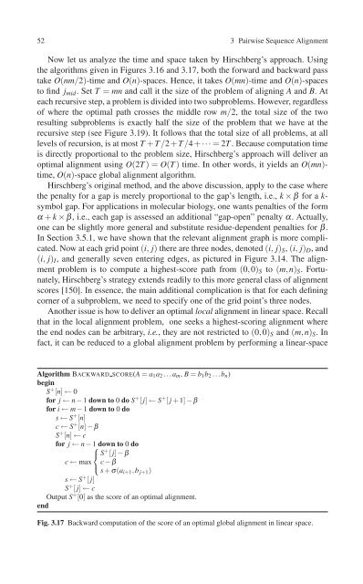
Algorithm BACKWARD SCORE(A = a 1 a 2 ...a m , B = b 1 b 2 ...b n )
begin
S + [n] ← 0
for j ← n − 1 down to 0 do S + [ j] ← S + [ j + 1] − β
for i ← m − 1 down to 0 do
s ← S + [n]
c ← S + [n] − β
S + [n] ← c
for j ← n − 1⎧
down to 0 do
⎨ S + [ j] − β
c ← max c − β
⎩
s + σ(a i+1 ,b j+1 )
s ← S + [ j]
S + [ j] ← c
Output S + [0] as the score of an optimal alignment.
end
Fig. 3.17 Backward computation of the score of an optimal global alignment in linear space.