Lecture Notes 19: Magnetic Fields in Matter I; Dia-/Para-/Ferro ...
Lecture Notes 19: Magnetic Fields in Matter I; Dia-/Para-/Ferro ...
Lecture Notes 19: Magnetic Fields in Matter I; Dia-/Para-/Ferro ...

Create successful ePaper yourself
Turn your PDF publications into a flip-book with our unique Google optimized e-Paper software.
UIUC Physics 435 EM <strong>Fields</strong> & Sources I Fall Semester, 2007 <strong>Lecture</strong> <strong>Notes</strong> <strong>19</strong> Prof. Steven Errede<br />
LECTURE NOTES <strong>19</strong><br />
MAGNETIC FIELDS IN MATTER<br />
THE MACROSCOPIC MAGNETIZATION, Μ <br />
There exist many types of materials which, when placed <strong>in</strong> an external magnetic field<br />
<br />
Bext<br />
( r ) become magnetized — i.e. at the microscopic level ∃ <strong>in</strong>ternal atomic/molecular magnetic<br />
dipole moments m atom<br />
or m <br />
molecular<br />
, which, <strong>in</strong> the presence of the external align<strong>in</strong>g magnetic field<br />
<br />
Bext<br />
( r ) produce magnetic torques τ ( r ) = m ( r ) × B <br />
ext ( r<br />
) which act on the <strong>in</strong>dividual<br />
atomic/molecular dipole moments, thereby caus<strong>in</strong>g a net alignment of the atomic/molecular<br />
<br />
magnetic dipole moments matom mmolecular<br />
which <strong>in</strong> turn results <strong>in</strong> a net, macroscopic magnetic<br />
polarization, also known as the magnetization, Μ <br />
( r ) . This is analogous to the situation<br />
associated with dielectric materials where electrostatic torques τ ( r ) = p ( r ) × E <br />
ext ( r<br />
) act on<br />
<br />
<strong>in</strong>dividual atomic/molecular electric dipole moments patom pmolecular<br />
<strong>in</strong> an external electric<br />
<br />
field Eext<br />
( r)<br />
result<strong>in</strong>g <strong>in</strong> a net, macroscopic electric polarization, Ρ <br />
( r ) .<br />
<br />
In the absence of an external applied magnetic field (i.e. Bext<br />
( r ) = 0) the macroscopic<br />
<br />
alignment of the atomic/molecular magnetic dipole moments matom mmolecular<br />
(<strong>in</strong> many, but not all<br />
magnetic materials) is random, due to fluctuations <strong>in</strong> the <strong>in</strong>ternal thermal energy of the material<br />
at f<strong>in</strong>ite temperature (e.g. room temperature). Thus, no net macroscopic magnetization<br />
<br />
M ( r ) exists <strong>in</strong> many such materials for Bext<br />
( r ) = 0 at f<strong>in</strong>ite (absolute) temperature, T.<br />
<br />
We def<strong>in</strong>e the macroscopic magnetic polarization (a.k.a. magnetization) M ( r ) of a magnetic<br />
material <strong>in</strong> complete analogy to that associated with the macroscopic electric polarization<br />
<br />
P( r ) of a dielectric material:<br />
<br />
Macroscopic Electric Polarization P( r ) :<br />
⎛electric dipole moment ⎞ <br />
P ( r)<br />
= ⎜ ⎟ at po<strong>in</strong>t r SI Units of P : Coulombs/m 2<br />
⎝ unit volume ⎠<br />
<br />
N<br />
<br />
N <br />
pmol ( r) ( ) ( )<br />
( )<br />
i i Qd<br />
i i<br />
ri<br />
P r = nmol<br />
pmol<br />
r ≡ ∑<br />
=<br />
Volume, V ∑ Volume, V<br />
n<br />
mol<br />
=<br />
# atoms/molecules<br />
unit volume<br />
i= 1 i=<br />
1<br />
<br />
Macroscopic <strong>Magnetic</strong> Polarization/Magnetization M ( r ) :<br />
⎛magnetic dipole moment ⎞ <br />
M ( r)<br />
= ⎜ ⎟ at po<strong>in</strong>t r SI Units of M : Amperes/meter<br />
⎝ unit volume ⎠<br />
N<br />
<br />
N <br />
mmol ( r) ( ) ( )<br />
( )<br />
i i Ia<br />
i i<br />
ri<br />
M r = nmol<br />
mmol<br />
r ≡ ∑<br />
=<br />
Volume, V ∑ Volume, V<br />
i= 1 i=<br />
1<br />
© Professor Steven Errede, Department of Physics, University of Ill<strong>in</strong>ois at Urbana-Champaign, Ill<strong>in</strong>ois<br />
2005-2008. All Rights Reserved.<br />
1
UIUC Physics 435 EM <strong>Fields</strong> & Sources I Fall Semester, 2007 <strong>Lecture</strong> <strong>Notes</strong> <strong>19</strong> Prof. Steven Errede<br />
Note that the magnetization ( r )<br />
<br />
K( r)<br />
(Amperes/meter), whereas the electric polarization P( r )<br />
surface charge density, σ ( r<br />
) (Coulombs/m 2 ).<br />
There are (at least) four k<strong>in</strong>ds of magnetism:<br />
1.) DIAMAGNETISM:<br />
Μ <br />
has SI units the same as that for a surface current density,<br />
has SI units the same as that for a<br />
The <strong>in</strong>duced macroscopic magnetization Μ <br />
( r ) is antiparallel to B ( r )<br />
dia<br />
<br />
ext<br />
. Due to the physics<br />
orig<strong>in</strong> of diamagnetism at the microscopic scale – i.e. at the atomic/molecular scale, ALL<br />
substances are diamagnetic! However, diamagnetism is very a weak phenomenon – other k<strong>in</strong>ds<br />
of magnetism (see below) can “over-ride”/mask out the diamagnetic behavior of a material.<br />
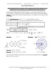
<strong>Dia</strong>magnetism results from changes <strong>in</strong>duced <strong>in</strong> the orbits of electrons <strong>in</strong> the atoms/molecules<br />
of a substance, due to the applied/external magnetic field. The direction of the change <strong>in</strong> orbital<br />
motion of the electrons is such that it to opposes the change <strong>in</strong> applied magnetic flux (this is<br />
noth<strong>in</strong>g more than Lenz’s Law act<strong>in</strong>g at the microscopic/atomic/molecular scale!).<br />
Superconductors are examples of strong diamagnets – they are <strong>in</strong> fact perfect diamagnets,<br />
<br />
Bext<br />
r (* if no flux-p<strong>in</strong>n<strong>in</strong>g<br />
Μ <br />
dia<br />
r vanishes when<br />
<br />
B r = .<br />
completely* screen<strong>in</strong>g out the applied external magnetic field ( )<br />
defects are present <strong>in</strong> the superconduct<strong>in</strong>g material). Note that ( )<br />
ext<br />
( ) 0<br />
2.) PARAMAGNETISM:<br />
The <strong>in</strong>duced macroscopic magnetization, Μ <br />
para ( r ) is parallel to Bext<br />
( r ) . Atoms or molecules<br />
that have a net orbital and/or <strong>in</strong>tr<strong>in</strong>sic sp<strong>in</strong> magnetic dipole moment m (e.g. atoms/molecules<br />
with unpaired electrons – such as A<br />
, Ba, Ca, Na, Sr, U,<br />
… and also metals – due to the<br />
magnetic dipole moments m associated with <strong>in</strong>tr<strong>in</strong>sic sp<strong>in</strong>s of the conduction electrons) are<br />
<br />
paramagnetic materials. The external applied magnetic field Bext<br />
( r ) exerts a torque on these<br />
atomic/molecular magnetic dipole moments m which tends to (partially) align them, giv<strong>in</strong>g rise<br />
to a net Μ <br />
para ( r ) which is parallel to Bext<br />
( r ) . The energy of alignment UM<br />
( r ) =−m ( r ) i Bext<br />
( r )<br />
is a m<strong>in</strong>imum when m <br />
is parallel to Bext<br />
( r ) . This is analogous to the net <strong>in</strong>duced electric<br />
polarization Ρ <br />
( r ) which is parallel to Eext<br />
( r ) <strong>in</strong> dielectric materials, the energy of alignment<br />
<br />
UE( r) =−p( r) iEext( r)<br />
when p <br />
is parallel to Eext<br />
( r)<br />
. Note that Μ <br />
para ( r ) also vanishes<br />
<br />
when B ( r ) = 0.<br />
ext<br />
Μ <br />
Μ <br />
dia<br />
para<br />
<br />
( r )<br />
<br />
( r )<br />
<br />
B<br />
<br />
B<br />
ext<br />
ext<br />
<br />
( r )<br />
<br />
( r )<br />
2<br />
© Professor Steven Errede, Department of Physics, University of Ill<strong>in</strong>ois at Urbana-Champaign, Ill<strong>in</strong>ois<br />
2005-2008. All Rights Reserved.
UIUC Physics 435 EM <strong>Fields</strong> & Sources I Fall Semester, 2007 <strong>Lecture</strong> <strong>Notes</strong> <strong>19</strong> Prof. Steven Errede<br />
Μ <br />
depends on the (entire)<br />
!! There exists a non-l<strong>in</strong>ear hysteresis-type relation between<br />
3.) FERROMAGNETISM: The macroscopic magnetization,<br />
ferro ( r )<br />
<br />
past history of exposure to Bext<br />
( r )<br />
Μ <br />
( r ) and B ( r )<br />
<br />
ferro<br />
ext . Iron and other ferromagnetic materials have a “macroscopic” crystall<strong>in</strong>e<br />
doma<strong>in</strong> structure (a typical scale length <strong>in</strong>volves many thousands of atoms), with<strong>in</strong> a doma<strong>in</strong><br />
(nearly) all of the atomic/molecular magnetic dipole moments m are aligned parallel to each<br />
other ⇒Μ <br />
doma<strong>in</strong> ( r ) can be very large. However, the orientation of Μ <br />
doma<strong>in</strong><br />
over many doma<strong>in</strong>s is<br />
<br />
≈ random, unless B ( r) ≠ 0 . However, ferromagnetic materials have a critical temperature<br />
ext<br />
(known as the Curie Temperature T<br />
C<br />
) below which the doma<strong>in</strong>s can spontaneously align − a<br />
phase transition occurs <strong>in</strong> the material at this temperature! In the presence of an external applied<br />
magnetic field B <br />
ext<br />
the alignment of ferromagnetic doma<strong>in</strong>s tends to be parallel to B <br />
ext<br />
, but it is <strong>in</strong><br />
fact (more) complicated than this, because it it history dependent!!! The alignment arises from<br />
quantum mechanics – <strong>in</strong>tr<strong>in</strong>sic sp<strong>in</strong> and the Pauli exclusion pr<strong>in</strong>ciple. Thus, Μ <br />
ferro ( r ) does not<br />
<br />
vanish when B ( r ) = 0!!!<br />
ext<br />
History-Dependence / Hysteresis Relation Between Μ <br />
ferro<br />
and B <br />
ext<br />
for <strong>Ferro</strong>magnetic Materials<br />
for T < T (= Curie Temperature):<br />
C<br />
<strong>Ferro</strong>magnetic behavior vanishes for T > TC<br />
The material then becomes paramagnetic.<br />
The arrows <strong>in</strong>dicate the path taken for Μ <br />
ferro<br />
: B <br />
ext<br />
starts at B<br />
ext<br />
= 0 , then goes to B <br />
max<br />
, then<br />
through 0, go<strong>in</strong>g to B m<strong>in</strong><br />
, then through 0 aga<strong>in</strong> and then go<strong>in</strong>g to B<br />
max<br />
, etc….<br />
4.) ANTI-FERROMAGNETISM (a.k.a. FERRIMAGNETISM)<br />
In some magnetically-ordered materials ∃ an anti-parallel alignment of <strong>in</strong>tr<strong>in</strong>sic sp<strong>in</strong>s, due to<br />
two (or more) <strong>in</strong>ter-penetrat<strong>in</strong>g crystall<strong>in</strong>e structures, such that no spontaneous magnetization <strong>in</strong><br />
the bulk material occurs. Ferrimagnetism/antiferromagnetism occurs for temperatures T < T Ne ' el<br />
.<br />
Materials exhibit<strong>in</strong>g antiferromagnetic properties are relatively uncommon – e.g. URu 2 Si 2 .<br />
© Professor Steven Errede, Department of Physics, University of Ill<strong>in</strong>ois at Urbana-Champaign, Ill<strong>in</strong>ois<br />
2005-2008. All Rights Reserved.<br />
3
UIUC Physics 435 EM <strong>Fields</strong> & Sources I Fall Semester, 2007 <strong>Lecture</strong> <strong>Notes</strong> <strong>19</strong> Prof. Steven Errede<br />
FORCES & TORQUES ON MAGNETIC DIPOLES<br />
When a magnetic dipole with magnetic dipole moment m is placed <strong>in</strong> an external magnetic<br />
field B <br />
ext<br />
a torque on the magnetic dipole τ<br />
M<br />
= m× B<br />
<br />
ext will occur, just as we saw for the case of<br />
an electric dipole with electric dipole moment p when it is placed <strong>in</strong> an external electric field<br />
E <br />
giv<strong>in</strong>g rise to a torque on the electric dipoleτ E<br />
= p×<br />
E ext .<br />
ext<br />
As we also learned for the case of an electric dipole <strong>in</strong> a uniform external electric field,<br />
similarly, for a magnetic dipole placed <strong>in</strong> a uniform external magnetic field, there is no net force<br />
act<strong>in</strong>g on the magnetic dipole.<br />
For a magnetic dipole with magnetic dipole moment m (e.g. aris<strong>in</strong>g from a current loop)<br />
placed <strong>in</strong> an uniform external magnetic field B <br />
ext<br />
the net force on the is zero:<br />
F<br />
net<br />
I d <br />
( r <br />
) B <br />
m ext( r <br />
) I ( d <br />
( r <br />
)) B <br />
= ∫<br />
′ ′ × ′ = ′ ′ ×<br />
ext( r <br />
<br />
<br />
′)<br />
= 0<br />
C′ ∫ <br />
C′<br />
<br />
cf w/ that for an electric dipole placed <strong>in</strong> a uniform external electric field E ext<br />
:<br />
<br />
net <br />
F<br />
= F r + F r = qE r − qE r = q E r − E r =<br />
≡ 0<br />
( ) 0<br />
( ) ( ) ( ) ( ) ( ) ( )<br />
p + + − − ext + ext − ext + ext −<br />
<br />
The nature of the magnetic (electric) torque τ<br />
M<br />
= m× B<br />
<br />
ext ( τ<br />
E<br />
= p × Eext)<br />
is such that it tends<br />
<br />
to align m( p)<br />
with (i.e. parallel to) the applied/external B ext ( E <br />
ext ) respectively.<br />
<br />
⇒ The effect(s) of magnetic torque expla<strong>in</strong>s paramagnetism, with Μ<br />
para<br />
Bext<br />
. One might be<br />
tempted to believe that paramagnetism should be a universal phenomenon, common to all<br />
materials. However, paramagnetism is connected to the <strong>in</strong>tr<strong>in</strong>sic magnetic dipole moment of an<br />
unpaired electron and/or its orbital magnetic dipole moment. Because of the Pauli exclusion<br />
pr<strong>in</strong>ciple (identical fermions, here, electrons) cannot be <strong>in</strong> the exact same quantum state, hence<br />
pairs of electrons can only be <strong>in</strong> the same quantum state with one of them sp<strong>in</strong>-up, and the other<br />
sp<strong>in</strong> down. Thus, torques on paired magnetic dipole moments (or more correctly, the B -fields<br />
associated with the paired electron magnetic dipole moments m ) cancel.<br />
⇒ <strong>Para</strong>magnetism only arises <strong>in</strong> atoms/molecules with an odd number of electrons – the<br />
outermost electron is unpaired ⇒ hence it (alone) is subject to magnetic torque(s).<br />
As we saw <strong>in</strong> the case for an electric dipole with electric dipole moment p <strong>in</strong> a non-uniform<br />
external electric field E <br />
ext<br />
, a non-zero force acts on the electric dipole. Similarly, for a magnetic<br />
dipole, with magnetic dipole moment m <strong>in</strong> a non-uniform external magnetic<br />
field B <br />
ext<br />
experiences a non-zero force:<br />
<br />
F<br />
m<br />
r m r Bext r m r Bext<br />
r<br />
<br />
F<br />
r p r E r p r E r<br />
( ) ( ( ) ) ( )<br />
( ) ( ( ) ) ( )<br />
( ) =∇ ( ) i ( ) = i ∇ {last step valid iff m( r)<br />
<br />
( ) =∇<br />
<br />
( ) i<br />
<br />
( ) =<br />
<br />
i ∇<br />
<br />
{last step valid iff p ( r )<br />
p ext ext<br />
e<br />
= constant vector}<br />
= constant vector}<br />
4<br />
© Professor Steven Errede, Department of Physics, University of Ill<strong>in</strong>ois at Urbana-Champaign, Ill<strong>in</strong>ois<br />
2005-2008. All Rights Reserved.
UIUC Physics 435 EM <strong>Fields</strong> & Sources I Fall Semester, 2007 <strong>Lecture</strong> <strong>Notes</strong> <strong>19</strong> Prof. Steven Errede<br />
Similarly, work (= potential energy) of a magnetic (electric) dipole moment <strong>in</strong> an external<br />
<br />
magnetic (electric) field, Bext<br />
( Eext<br />
) are (respectively) given by:<br />
<br />
<br />
W<br />
= PE . . =−m i B vs. W<br />
= PE . . =−p i E<br />
m m ext<br />
p p ext<br />
The Physics of <strong>Dia</strong>magnetism<br />
Atomic electrons orbit/revolve around the nucleus of the atom at some mean / average /<br />
characteristic radius, R. Atomic electrons bound to the nucleus of an atom no longer behave like<br />
po<strong>in</strong>t-like particles, but as quantum-mechanical matter waves. However, an orbit<strong>in</strong>g atomic<br />
electron “wave” still constitutes a circulat<strong>in</strong>g current:<br />
I<br />
QM<br />
eve eve eve<br />
~ = = λe C = 2π<br />
R for ground state<br />
λ C 2πR<br />
e<br />
Gnd State<br />
Gnd State<br />
Conventional<br />
Current, I<br />
ẑ<br />
<br />
B<br />
ext<br />
= Bzˆ<br />
o<br />
R<br />
<br />
m<br />
e<br />
<br />
v<br />
e<br />
=−m zˆ<br />
e<br />
e −<br />
= vϕˆ<br />
e<br />
Classically, a circulat<strong>in</strong>g po<strong>in</strong>t electric charge has:<br />
I<br />
Class<br />
e<br />
= with τ 2<br />
orbit<br />
= C = π R<br />
τ<br />
ve<br />
v<br />
⇒<br />
e<br />
orbit<br />
I<br />
Class<br />
eve<br />
= = I<br />
2π R<br />
QM<br />
⎛ ev<br />
Then: m= Ia =− e<br />
⎞<br />
⎜ ⎟<br />
⎝2π<br />
R ⎠<br />
π 2 1<br />
R zˆ<br />
=− ( ev ) ˆ<br />
eR z<br />
2<br />
due to e − charge<br />
<br />
With no external magnetic field applied B<br />
ext<br />
= 0, thus the forces act<strong>in</strong>g on the atomic electron are:<br />
<br />
Felectrostatic<br />
= Fcentripetal<br />
2<br />
2<br />
2<br />
2<br />
1 Ze <br />
ve<br />
1 Ze v<br />
− ˆ<br />
ˆ<br />
2 r =− m<br />
e a<br />
centipetal<br />
=− m<br />
e r ⇒ Equation A:<br />
2 r<br />
e<br />
ˆ=<br />
m ˆ<br />
e r<br />
4πε<br />
R<br />
R<br />
4πε<br />
R R<br />
o<br />
e<br />
m = mass of electron<br />
Z = nuclear electric charge # {+Ze = nuclear charge}<br />
o<br />
© Professor Steven Errede, Department of Physics, University of Ill<strong>in</strong>ois at Urbana-Champaign, Ill<strong>in</strong>ois<br />
2005-2008. All Rights Reserved.<br />
5
UIUC Physics 435 EM <strong>Fields</strong> & Sources I Fall Semester, 2007 <strong>Lecture</strong> <strong>Notes</strong> <strong>19</strong> Prof. Steven Errede<br />
<br />
With an external magnetic field present Bext<br />
≠ 0, thus the forces act<strong>in</strong>g on the atomic electron are:<br />
<br />
net<br />
FEM = Felectrostatic + FB = F′<br />
centripetal<br />
<br />
2<br />
net<br />
1 Ze <br />
F ˆ<br />
EM<br />
= Felectrostatic + FB =− r− e<br />
2 ( ve × Bext<br />
)<br />
4πε<br />
o<br />
R<br />
<br />
Suppose ˆ <br />
Bext<br />
= Bz<br />
0<br />
and v ˆ<br />
e<br />
= vϕ<br />
e<br />
(as shown <strong>in</strong> above pix)<br />
ˆ ϕ × zˆ = ˆ ϕ× cosθrˆ<br />
− s<strong>in</strong>θθˆ<br />
<br />
θ = 90<br />
rˆ<br />
× ˆ θ = ˆ ϕ<br />
ˆ θ× ˆ ϕ = rˆ<br />
ˆ ϕ × rˆ<br />
= ˆ θ<br />
Then:<br />
Then: ( )<br />
( ˆr )<br />
=− ˆ ϕ× ˆ θ =− − = + ˆr<br />
2<br />
net 1 Ze<br />
<br />
v′<br />
2<br />
e<br />
ˆ<br />
EM<br />
=− −ev′<br />
2 eBor<br />
= ′<br />
centripetal<br />
=−<br />
e<br />
4πε<br />
o<br />
R<br />
R<br />
F<br />
F m rˆ<br />
<br />
s<strong>in</strong>θ<br />
= s<strong>in</strong> 90 = 1<br />
<br />
cosθ<br />
= cos90 = 0<br />
<br />
2<br />
2<br />
1 Ze<br />
v′<br />
e<br />
Then for Bext<br />
≠ 0 we have Equation B: + ev′<br />
2 eBo = me<br />
4πε<br />
o<br />
R<br />
R<br />
Note that s<strong>in</strong>ce we have an additional term on LHS of Equation B, then we see that:<br />
<br />
<br />
v′ B ≠0 ≠ v B = 0 .<br />
( ) ( )<br />
e ext e ext<br />
Subtract Equation A from Equation B:<br />
e 2 2<br />
ev′ <br />
eB0<br />
= m ( v′<br />
e<br />
−ve<br />
)<br />
0<br />
R <br />
for<br />
<br />
⇒ v′<br />
ˆ<br />
e<br />
> ve Bext<br />
=+ B z<br />
> 0<br />
If the change <strong>in</strong> ,<br />
e<br />
But: ve ve ve<br />
ˆ θ × rˆ<br />
=−ˆ<br />
ϕ<br />
ˆ ϕ× ˆ θ =−rˆ<br />
rˆ<br />
× ˆ ϕ =−ˆ<br />
θ<br />
> 0<br />
( v′ for ˆ<br />
e<br />
< ve Bext<br />
=−B0 z)<br />
v Δv ≡( v′<br />
− v ) is small, then: v′ 2 − v 2 = ( v′ − v )( v′ + v ) =Δ v ( v′<br />
+ v )<br />
e e e<br />
′ = +Δ (s<strong>in</strong>ce v ( v′<br />
v )<br />
Δ ≡ − )<br />
e e e<br />
2 2<br />
∴ v′ e<br />
− ve =Δ ve( ( ve +Δ ve)<br />
+ ve) =Δ ve( ve +Δ ve + ve) =Δ ve( 2ve +Δ ve)<br />
= 2v Δ v +Δv 2v Δv<br />
e e<br />
2<br />
e e e<br />
neglect<br />
m<br />
R<br />
e<br />
∴ ev′ B = e( v +Δv ) B ( v Δv<br />
)<br />
e 0 e e 0<br />
2<br />
e e<br />
2 v e<br />
me<br />
ve<br />
ev e<br />
B0<br />
Δ<br />
R<br />
eBo<br />
R<br />
or: Δve<br />
<br />
2m<br />
e<br />
e e e e e e e e e<br />
<br />
6<br />
© Professor Steven Errede, Department of Physics, University of Ill<strong>in</strong>ois at Urbana-Champaign, Ill<strong>in</strong>ois<br />
2005-2008. All Rights Reserved.
UIUC Physics 435 EM <strong>Fields</strong> & Sources I Fall Semester, 2007 <strong>Lecture</strong> <strong>Notes</strong> <strong>19</strong> Prof. Steven Errede<br />
But if:<br />
eve<br />
ev′<br />
e<br />
I = and I′ = and v′<br />
e<br />
> v<br />
2πR<br />
2πR<br />
Then:<br />
e( v′ e<br />
− ve)<br />
eΔve<br />
Δ I = I′<br />
− I = = but:<br />
2π<br />
R 2π<br />
R<br />
∴<br />
2<br />
2<br />
eBo<br />
R eBo<br />
Δ I = =<br />
4 π me<br />
R 4π me<br />
Δ I =<br />
2<br />
eB0<br />
π m<br />
Then:<br />
4<br />
e<br />
m Ia Iπ<br />
R<br />
2<br />
= = and<br />
′ ′<br />
m′ Ia ′ I′π<br />
R<br />
e<br />
eBo<br />
R<br />
Δve<br />
<br />
2m<br />
2<br />
2<br />
= = ( a=<br />
π R )<br />
2<br />
Thus: Δ m= m − m= ( I − I) a=Δ Ia=Δ<br />
Iπ<br />
R<br />
2<br />
2<br />
⎛ eB<br />
∴ Δ m=Δ Iπ<br />
R = o<br />
⎜<br />
⎝4<br />
π me<br />
<br />
But recall that m=−mzˆ<br />
⎞<br />
⎟ π R<br />
⎠<br />
2<br />
eBR<br />
=<br />
4m<br />
2 2<br />
o<br />
e<br />
e<br />
Therefore:<br />
i.e. m po<strong>in</strong>ts down.<br />
2 2<br />
eBR <br />
o<br />
Δ m=− zˆ,<br />
B ˆ<br />
ext<br />
= Bo<br />
z<br />
4m<br />
e<br />
Or:<br />
2 2<br />
⎛eR<br />
⎞ <br />
Δ m=−⎜ ⎟B<br />
⎝ 4me<br />
⎠<br />
ext<br />
The po<strong>in</strong>t is, that for diamagnetic materials, the change <strong>in</strong> the magnetic dipole moment m , Δm<br />
<br />
is opposite to the direction of B <br />
ext<br />
- i.e. if B ˆ<br />
ext<br />
= Bz<br />
o<br />
<strong>in</strong>creases, then m also <strong>in</strong>creases, but <strong>in</strong> the<br />
opposite direction to try to cancel/buck the external/applied magnetic field, B <br />
ext<br />
. This is a<br />
simply a manifestation of Lenz’s Law at the atomic scale!!!<br />
This is what phenomenon of diamagnetism is due to, at least from a ≈ semi-classical perspective.<br />
The <strong>in</strong>duced dipole moments <strong>in</strong> diamagnetic materials (essentially every material) po<strong>in</strong>t <strong>in</strong> the<br />
direction opposite to the applied magnetic field. The macroscopic magnetization Μ result<strong>in</strong>g<br />
from diamagnetism is relatively speak<strong>in</strong>g very small. <strong>Dia</strong>magnetism (except <strong>in</strong> superconductors)<br />
is extremely weak.<br />
© Professor Steven Errede, Department of Physics, University of Ill<strong>in</strong>ois at Urbana-Champaign, Ill<strong>in</strong>ois<br />
2005-2008. All Rights Reserved.<br />
7
UIUC Physics 435 EM <strong>Fields</strong> & Sources I Fall Semester, 2007 <strong>Lecture</strong> <strong>Notes</strong> <strong>19</strong> Prof. Steven Errede<br />
<br />
THE MAGNETIC VECTOR POTENTIAL Ar ( ) , THE MAGNETIC FIELD B( r)<br />
=∇× A( r)<br />
OF A MAGNETIZED OBJECT WITH MAGNETIZATION Μ <br />
( r )<br />
<br />
Recall that the magnetic vector potential Ar ( ) of a magnetic dipole with magnetic dipole<br />
2<br />
moment ( Amp-m )<br />
m <br />
is:<br />
<br />
⎛ μo<br />
⎞m×<br />
rˆ<br />
Adipole<br />
( r) = ⎜ ⎟ 2<br />
⎝4π<br />
⎠ r<br />
{SI Units: Tesla-meters = Newtons/Ampere = F/I !!!}<br />
Thus, <strong>in</strong> a magnetized object with macroscopic magnetization<br />
(magnetic dipole moment per unit volume) Μ <br />
( r′ ) , each volume<br />
element dτ ′with<strong>in</strong> the volume v′ has a magnetic dipole moment<br />
<br />
m r′ =Μ <br />
r′ dτ ′.<br />
associated with it of: ( ) ( )<br />
Thus, the <strong>in</strong>f<strong>in</strong>itesimal contribution to the magnetic vector<br />
<br />
Ar<br />
m r′<br />
<br />
potential ( ) due to the magnetic dipole moment ( )<br />
associated with the macroscopic magnetization Μ <br />
( r′ ) <strong>in</strong> the<br />
<strong>in</strong>f<strong>in</strong>itesimal volume element dτ ′is:<br />
<br />
<br />
<br />
<br />
⎛ μ m( r ) ˆ ( r ) d ˆ<br />
o ⎞ ′ × r ⎛ μ Μ ′ τ ′ ×<br />
o ⎞ r<br />
dA( r ) = ⎜ ⎟ =<br />
2 ⎜ ⎟ 2<br />
⎝4π<br />
⎠ r ⎝4π<br />
⎠ r<br />
<br />
with r = r − r′<br />
<br />
Then the total magnetic vector potential Ar ( ) is obta<strong>in</strong>ed by <strong>in</strong>tegrat<strong>in</strong>g this expression over the<br />
entire volume v′ of the magnetized material:<br />
<br />
<br />
<br />
⎛ μ ( r ) d ˆ<br />
o ⎞ Μ ′ τ ′ × r<br />
Ar ( ) = ∫ dAr ( ) =<br />
v′ ⎜ ⎟<br />
2<br />
4π<br />
∫v′<br />
⎝ ⎠ r<br />
⎛1⎞<br />
1 rˆ<br />
Now aga<strong>in</strong>: ∇ ′ ⎜ ⎟=∇ ′ =<br />
2<br />
⎝ r ⎠ r − r′<br />
r<br />
⎛ μ ⎞ ⎡ ⎛ 1 ⎞⎤<br />
Ar = ⎜ Μ r′ × ∇′ dτ<br />
′<br />
4π ⎟ ∫v′<br />
⎢ ⎜ ⎟⎥<br />
⎝ ⎠ ⎣ ⎝ r ⎠⎦<br />
<br />
∇× fA = f ∇× A − A× ∇f<br />
o<br />
Thus: ( ) ( )<br />
Integrat<strong>in</strong>g by parts, and us<strong>in</strong>g ( ) ( ) ( )<br />
<br />
μ ⎧<br />
<br />
⎛ ⎞⎪ 1 ⎡Μ<br />
( r′<br />
) ⎤ ⎫⎪<br />
Ar = ⎜ ⎨ ∇ ′ ×Μ r′ ⎤dτ<br />
′ − ∇ ′ × ⎢ ⎥dτ<br />
′ ⎬<br />
4π ⎟ ∫v′ ⎣ ⎦ ∫v′<br />
⎝ ⎠⎪ ⎩<br />
r<br />
⎣ r ⎦ ⎪⎭<br />
o<br />
Then: ( ) ⎡ ( )<br />
∫<br />
Then us<strong>in</strong>g: V ( r) dτ<br />
V ( r) da V( r)<br />
v<br />
<br />
∇× =− ∫ × =<br />
S<br />
(See Griffiths Problem 1.60 (b), page 56)<br />
:<br />
( Arbitrary Vector Po<strong>in</strong>t Function)<br />
8<br />
© Professor Steven Errede, Department of Physics, University of Ill<strong>in</strong>ois at Urbana-Champaign, Ill<strong>in</strong>ois<br />
2005-2008. All Rights Reserved.
UIUC Physics 435 EM <strong>Fields</strong> & Sources I Fall Semester, 2007 <strong>Lecture</strong> <strong>Notes</strong> <strong>19</strong> Prof. Steven Errede<br />
Ar<br />
μ 1 1<br />
= ⎛ ⎞⎧ ⎡∇ ⎨ ′ ×Μ 4π r <br />
′ ⎤ d ′ + ⎡Μ <br />
r <br />
′ × da <br />
⎜ ⎟ ′ ⎤⎬<br />
⎫<br />
v′ ⎣ ⎦<br />
s′<br />
⎩ r<br />
<br />
r ⎣ ⎦<br />
⎭<br />
o<br />
Thus: ( ) ( ) τ ( )<br />
But:<br />
<br />
da′ = nda ˆ ′<br />
⎝ ⎠ ∫ ∫<br />
μ 1 <br />
o<br />
μo<br />
1<br />
Then: Ar ( ) ⎡<br />
<br />
<br />
= ( r)<br />
dτ<br />
( r)<br />
nˆ<br />
da ABound<br />
( r)<br />
4π∫<br />
∇ ′ ×Μ ′ ⎤ ′ + ⎡Μ ′ × ⎤ ′ =<br />
v′ r ⎣ ⎦ 4π<br />
∫S′<br />
⎣ ⎦<br />
<br />
r <br />
<br />
<br />
≡ JBound( r′ )<br />
≡ KBound( r′<br />
)<br />
<br />
<br />
<br />
<br />
<br />
μ JBound<br />
( r′ o<br />
) μ K<br />
o Bound ( r′<br />
) <br />
Or: ABound<br />
( r)<br />
= dτ<br />
′ +<br />
da′<br />
4π∫v′ r 4π∫<br />
with r = r −r′<br />
S′<br />
r<br />
<br />
Compare this result to that which we obta<strong>in</strong>ed for the magnetic vector potential Ar ( ) associated<br />
<br />
with a free volume current density J<br />
free ( r′ ) and a free surface/sheet current density K<br />
free ( r′ )<br />
(see P435 <strong>Lecture</strong> <strong>Notes</strong> 16, page 6):<br />
<br />
<br />
μ J<br />
free ( r′ ) K<br />
free ( r )<br />
o<br />
μ ′<br />
o<br />
<br />
Afree<br />
( r)<br />
= dτ<br />
′ +<br />
da′<br />
4π∫v′ r 4π∫<br />
with r = r −r′<br />
S′<br />
r<br />
Thus for a magnetized material with macroscopic magnetization (magnetic dipole moment per<br />
unit volume) Μ <br />
( r′ ) conta<strong>in</strong>ed with<strong>in</strong> <strong>in</strong> the enclos<strong>in</strong>g source volume v′ bounded by the surface<br />
aris<strong>in</strong>g from the sum total of<br />
S′ , the magnetic vector potential at the field/observation po<strong>in</strong>t Ar ( )<br />
the macroscopic magnetization ( r′ )<br />
<br />
contributions from an equivalent bound volume current density JBound<br />
( r′ ) ≡∇ ′ ×Μ( r′<br />
)<br />
<br />
equivalent bound surface current density K ( r′ ) ≡Μ ( r′<br />
) × nˆ<br />
Μ present <strong>in</strong> the material can be equivalently represented by<br />
Bound<br />
normal at the surface of the magnetized material.<br />
surface<br />
and an<br />
where ˆn = outward unit<br />
On the <strong>in</strong>terior of the magnetized material:<br />
<br />
JBound<br />
( r′ ) ≡∇ ′ ×Μ( r′<br />
) = equivalent bound volume current density, SI units = Amps/m2<br />
<br />
2<br />
Amps / m<br />
1/ m<br />
Amps / m<br />
On the surface(s) of the magnetized material:<br />
<br />
K ( ) ( ) ˆ<br />
Bound<br />
r′ ≡Μ r′<br />
× n = equivalent bound surface current density, SI units = Amps/m<br />
<br />
Then: ( )<br />
Amps / m Amps / m<br />
<br />
<br />
<br />
<br />
<br />
μ J<br />
o Bound ( r′ ) μ K<br />
o Bound ( r′<br />
) <br />
ABound<br />
r = dτ<br />
′ +<br />
da′<br />
4π∫v′ r 4π∫<br />
with r = r − r′<br />
S′<br />
r<br />
© Professor Steven Errede, Department of Physics, University of Ill<strong>in</strong>ois at Urbana-Champaign, Ill<strong>in</strong>ois<br />
2005-2008. All Rights Reserved.<br />
9
UIUC Physics 435 EM <strong>Fields</strong> & Sources I Fall Semester, 2007 <strong>Lecture</strong> <strong>Notes</strong> <strong>19</strong> Prof. Steven Errede<br />
MAGNETIC MATERIALS<br />
<br />
JBound<br />
( r′ ) ≡∇×Μ( r′<br />
)<br />
<br />
K r′ ≡Μ r′<br />
× n<br />
Bound<br />
( ) ( ) ˆ<br />
surface<br />
DIELECTRIC MATERIALS<br />
<br />
ρ<br />
Bound<br />
r′ =−∇Ρ i r′<br />
<br />
σ r′ =Ρ <br />
r′<br />
i n<br />
⇔ ( ) ( )<br />
⇔ ( ) ( ) ˆ<br />
Bound<br />
surface<br />
So aga<strong>in</strong>, <strong>in</strong>stead of <strong>in</strong>tegrat<strong>in</strong>g over the macroscopic magnetization Μ <br />
( r′ ) (or polarization<br />
Ρ <br />
( r′ ) ) aris<strong>in</strong>g from the direct contributions from the <strong>in</strong>f<strong>in</strong>itesimal magnetic (and/or electric)<br />
<br />
<br />
dipoles m( r′ ) (and/or p ( r′ )), we replace these by macroscopic bound volume and surface<br />
<br />
<br />
current distributions JBound<br />
( r′ ) and KBound<br />
( r′<br />
) (and/or ρ<br />
Bound ( r′<br />
) and σ<br />
Bound ( r<br />
′)<br />
); we can then<br />
<br />
obta<strong>in</strong> Ar ( ) (and/or V ( r <br />
)). Once Ar ( ) (and/or V ( r ) ) is known, we can then obta<strong>in</strong> B ( r )<br />
B <br />
( r) =∇× <br />
A <br />
( r)<br />
(and/or E( r)<br />
from ( <br />
E r)<br />
=−∇V<br />
( r)<br />
) !<br />
Note that for a magnetized material with macroscopic magnetization Μ <br />
( r′ ) we can also<br />
obta<strong>in</strong> the equivalent bound current, IBound<br />
from:<br />
<br />
<br />
I = J r′ da′ + K r′ d<br />
′<br />
∫<br />
( ) ( )<br />
∫<br />
Bound Bound Bound surface<br />
S⊥′ ⊥<br />
⊥<br />
C⊥′<br />
surface<br />
from<br />
Consider the equivalent bound surface current K <br />
Bound<br />
associated with a th<strong>in</strong> slab of<br />
<br />
magnetized material that has been placed <strong>in</strong> uniform magnetic field B ˆ<br />
ext<br />
= Bz<br />
o<br />
, <strong>in</strong> turn produc<strong>in</strong>g<br />
a uniform macroscopic magnetization (magnetic dipole per unit volume) Μ <br />
=Μ z ˆ<br />
o<br />
. At the<br />
microscopic level, atoms and/or molecules will tend to have their <strong>in</strong>duced and/or permanent<br />
magnetic dipole moments l<strong>in</strong>ed up parallel/anti-parallel to B <br />
ext<br />
for paramagnetic / diamagnetic<br />
materials, respectively. Suppose that the material is paramagnetic, as shown <strong>in</strong> the figure below:<br />
<br />
B ˆ<br />
ext<br />
= Bz<br />
o<br />
produces<br />
m= Ia = Iazˆ<br />
uniform magnetization<br />
Μ <br />
=Μ z ˆ<br />
o<br />
It can be seen from the above figure that on the <strong>in</strong>terior of the uniformly magnetized material<br />
the atomic/molecular microscopic currents will cancel each other (for uniform magnetization,<br />
Μ=Μ <br />
z ˆ<br />
o<br />
) except on the periphery (i.e. the surface) of the magnetic material.<br />
For uniformly magnetized material(s), e.g. Μ <br />
=Μ z<br />
<br />
ˆ J r ≡ ∇×Μ r =∇× Μ zˆ = 0<br />
o<br />
.<br />
: ( ) ( ) ( )<br />
Bound<br />
o<br />
10<br />
© Professor Steven Errede, Department of Physics, University of Ill<strong>in</strong>ois at Urbana-Champaign, Ill<strong>in</strong>ois<br />
2005-2008. All Rights Reserved.
UIUC Physics 435 EM <strong>Fields</strong> & Sources I Fall Semester, 2007 <strong>Lecture</strong> <strong>Notes</strong> <strong>19</strong> Prof. Steven Errede<br />
I<br />
K r <br />
= ∫<br />
′ d ′ for uniform magnetization, e.g. Μ=Μ <br />
z ˆ<br />
o<br />
.<br />
Then: ( )<br />
Bound Bound surface<br />
C⊥′<br />
⊥<br />
surface<br />
Example: Consider a cyl<strong>in</strong>drical rod of radius a and length of magnetized material immersed<br />
<br />
<strong>in</strong> a uniform B ˆ<br />
ext<br />
= Bz<br />
o<br />
as shown <strong>in</strong> the figure below. Then the magnetization is uniform, e.g.<br />
Μ=Μ<br />
<br />
z<br />
<br />
ˆ<br />
o<br />
. Thus, no equivalent bound volume current density JBound<br />
( r)<br />
exists, because<br />
<br />
J r =∇×Μ r =∇× Μ zˆ = 0 for uniform magnetization, Μ <br />
=Μ z ˆ<br />
o<br />
.<br />
Bound<br />
<br />
Μ=n m<br />
( ) ( ) ( )<br />
mol<br />
mol<br />
Uniform<br />
o<br />
Μ=Μ <br />
z ˆ<br />
o<br />
=Μ z ˆ<br />
a<br />
o<br />
<br />
Μ=<br />
<br />
Μ=<br />
<br />
m<br />
<br />
m<br />
Tot<br />
Tot<br />
Volume<br />
π a<br />
2<br />
ẑ<br />
bound<br />
<br />
B<br />
ext<br />
= Bzˆ<br />
produces uniform Μ=Μ <br />
z ˆ<br />
o<br />
K ( )<br />
o<br />
I<br />
K r <br />
= ∫<br />
′ d ′<br />
Bound<br />
C surface<br />
Bound ⊥ surface<br />
⊥′<br />
ŷ = K ˆ<br />
bound<br />
ϕ<br />
<br />
ˆϕ K = Μ× nˆ<br />
with nˆ<br />
= ˆ ρ<br />
<br />
m<br />
Tot<br />
= total dipole moment ˆx ˆρ =Μ ( ˆ ˆ)<br />
ˆ ˆ<br />
o<br />
z× ρ =Μ<br />
oϕ = Koϕ<br />
<br />
of magnetized ∴ I ˆ<br />
Bound<br />
= Kboundϕ =Μo<br />
ˆ, ϕ<br />
<br />
cyl<strong>in</strong>der i.e. K =Μ ˆ ϕ = K ˆ ϕ<br />
Bound<br />
surface<br />
Bound o o<br />
surface<br />
<br />
<br />
If Bext<br />
≠ uniform magnetic field, will result <strong>in</strong> a non-uniform magnetization, i.e. Μ≠uniform,<br />
<br />
which <strong>in</strong> turn also implies that the equivalent bound volume current density J<br />
Bound<br />
=∇×Μ≠0<br />
.<br />
This means that at microscopic level the atomic/molecular current loops no longer<br />
<br />
cancel each<br />
other (completely) <strong>in</strong> the <strong>in</strong>terior region of the magnetized material. Hence for Μ≠uniform:<br />
<br />
Volume<br />
<br />
JBound ( r′ ) =∇×Μ( r′ ) ≠0<br />
⇒ IBound =∫ JBound<br />
( r′<br />
) da<br />
′<br />
⊥<br />
Similarly, we also expect for non-uniform Μ that K ( r ) = Μ ( r ) × nˆ ≠0<br />
<br />
S⊥<br />
Bound<br />
<br />
′ ′<br />
surface<br />
and thus we<br />
will also have an equivalent bound surface current:<br />
then I Surface<br />
K <br />
Bound Bound ( r <br />
= ∫<br />
′)<br />
d ′<br />
′<br />
⊥ surface (for magnetized cyl<strong>in</strong>der <strong>in</strong> above figure: d ⊥′ = dz)<br />
C⊥<br />
surface<br />
Then us<strong>in</strong>g the pr<strong>in</strong>ciple of l<strong>in</strong>ear superposition:<br />
<br />
Tot Volume Surface<br />
<br />
I = I + I = J r′ da + K r′ d<br />
′<br />
∫<br />
( ) ( )<br />
Bound Bound Bound Bound Bound surface<br />
S⊥′ ⊥<br />
⊥<br />
C⊥′<br />
surface<br />
Note that these equivalent bound currents are flow<strong>in</strong>g <strong>in</strong> different places <strong>in</strong>/on the magnetized<br />
material – one is flow<strong>in</strong>g <strong>in</strong>side the material, the other is flow<strong>in</strong>g on the surface of the material.<br />
∫<br />
© Professor Steven Errede, Department of Physics, University of Ill<strong>in</strong>ois at Urbana-Champaign, Ill<strong>in</strong>ois<br />
2005-2008. All Rights Reserved.<br />
11
UIUC Physics 435 EM <strong>Fields</strong> & Sources I Fall Semester, 2007 <strong>Lecture</strong> <strong>Notes</strong> <strong>19</strong> Prof. Steven Errede<br />
<br />
<br />
( ) 0<br />
Note also that: ∇ i JBound<br />
( r) =∇× ∇×Μ ( r)<br />
= always <strong>in</strong> magnetostatics, because i J ( r)<br />
is the LHS of the Cont<strong>in</strong>uity Equation for equivalent bound currents (i.e. conservation of bound<br />
charge):<br />
<br />
<br />
∂ρBound<br />
( rt , )<br />
<br />
∇ i JBound<br />
( r, t)<br />
=− = 0 if ρBound<br />
( rt , ) ≠ fcn(t).<br />
∂t<br />
Note also that (here): ( )<br />
<br />
∇× ∇×Μ =∇ ∇ Μ −∇ Μ = 0<br />
2 <br />
( r ) ( ( r)<br />
) ( r)<br />
i i.e.: ∇∇Μ i ( r)<br />
{We will come back to this relation <strong>in</strong> the near future…}<br />
∇ <br />
Bound<br />
<br />
2 <br />
( ) =∇Μ( r)<br />
<br />
Griffiths Example 6.1:<br />
<br />
Determ<strong>in</strong>e the magnetic field B ( r ) associated with a uniformly magnetized sphere of radius R<br />
with uniform magnetization Μ=Μ <br />
z ˆ<br />
o<br />
as show <strong>in</strong> the figure below. Choose the local orig<strong>in</strong>ϑ<br />
to be at the center of the magnetized sphere:<br />
Μ=Μ<br />
<br />
z ˆ<br />
o<br />
ϑ<br />
ẑ<br />
ϕ<br />
θ<br />
ˆϕ<br />
ˆr<br />
ˆ θ<br />
P( r ) Field/Observation Po<strong>in</strong>t<br />
ŷ<br />
ˆϕ<br />
ˆx<br />
<br />
ˆ<br />
Bound<br />
= ∇×Μ =∇× Μ<br />
o<br />
= 0 .<br />
<br />
K r r n z r θ ϕ where: nˆ<br />
= rˆ<br />
S<strong>in</strong>ce the magnetization of the sphere is uniform, then: J ( r) ( r) ( z)<br />
However: ( ) =Μ ( ) × ˆ =Μ ( ˆ× ˆ) =Μ s<strong>in</strong> ˆ<br />
Bound<br />
surface<br />
o o<br />
Note: z rˆ ( rˆ ) rˆ ( rˆ)<br />
surface<br />
ˆ × = cosθ − s<strong>in</strong>θθˆ × = 0 − s<strong>in</strong>θ ˆ θ × =+ s<strong>in</strong> θ ˆ ϕ s<strong>in</strong>ce: rˆ× rˆ= 0, ˆ θ × rˆ=−<br />
ˆ ϕ<br />
Now recall that we learned <strong>in</strong> Griffiths Example 5.11 (p. 236-7)/P435 <strong>Lecture</strong> Note 16 p. 18-<strong>19</strong><br />
<br />
(the charged sp<strong>in</strong>n<strong>in</strong>g hollow sphere) that: K = σ v = σω × r′<br />
= σωRs<strong>in</strong><br />
ϕ ˆ ϕ<br />
free<br />
Uniformly Magnetized Sphere:<br />
<br />
K s<strong>in</strong> ˆ<br />
Bound<br />
=Μo<br />
θ ϕ<br />
<br />
2 2 <br />
B<strong>in</strong>side ( r < R)<br />
= μoΜ ozˆ<br />
= μoΜ<br />
3 3<br />
<br />
⎛ μo<br />
⎞ m<br />
B ( )<br />
3 ( 2cos ˆ s<strong>in</strong> ˆ<br />
outside<br />
r > R = ⎜ ⎟ θr+<br />
θθ )<br />
⎝4π<br />
⎠r<br />
4 <br />
3 4 3<br />
m= πR Μ = πR Μ ˆ<br />
oz<br />
3 3<br />
vs.<br />
Charged Sp<strong>in</strong>n<strong>in</strong>g Hollow Sphere:<br />
<br />
K s<strong>in</strong> ˆ<br />
free<br />
= σωR<br />
θϕ ⇒ Μ o<br />
= σωR<br />
<br />
2<br />
B<strong>in</strong>side<br />
r < R = μo<br />
σωR zˆ<br />
3<br />
<br />
⎛ μo<br />
⎞ m<br />
B 2cos ˆ s<strong>in</strong> ˆ<br />
outside<br />
r > R = ⎜ ⎟ θr+<br />
θθ<br />
3<br />
⎝4π<br />
⎠r<br />
4 4<br />
m= π R 3 σωR zˆ<br />
= π R 4 σωzˆ<br />
3 3<br />
⇐ ( ) ( )<br />
⇐ ( ) ( )<br />
vs. ( )<br />
12<br />
© Professor Steven Errede, Department of Physics, University of Ill<strong>in</strong>ois at Urbana-Champaign, Ill<strong>in</strong>ois<br />
2005-2008. All Rights Reserved.
UIUC Physics 435 EM <strong>Fields</strong> & Sources I Fall Semester, 2007 <strong>Lecture</strong> <strong>Notes</strong> <strong>19</strong> Prof. Steven Errede<br />
For magnetic media, we have obta<strong>in</strong>ed the follow<strong>in</strong>g relations:<br />
<br />
<br />
∂ρBound<br />
rt ,<br />
Bound current cont<strong>in</strong>uity equation: ∇ i JBound<br />
( r,<br />
t)<br />
=−<br />
∂t<br />
<br />
( )<br />
Equivalent bound volume current density JBound<br />
( r ) =∇×Μ( r<br />
) , where ( r )<br />
<br />
magnetic dipole moment per unit volume) Μ ( ) = ( ) = ( )<br />
<br />
Μ = magnetization (a.k.a.<br />
r nmo <br />
mmol r mTot<br />
r volumeand the<br />
<br />
KBound<br />
r = Μ r × n ≠ with correspond<strong>in</strong>g relations<br />
surface<br />
I Surface<br />
K r <br />
d<br />
Bound<br />
= ∫<br />
Bound<br />
<br />
⊥ surface<br />
equivalent bound surface current density ( ) ( ) ˆ 0<br />
<br />
Volume<br />
<br />
I<br />
Bound<br />
= ∫ JBound<br />
( r)<br />
da<br />
S⊥<br />
⊥<br />
and ( )<br />
C⊥<br />
surface<br />
Us<strong>in</strong>g the pr<strong>in</strong>ciple of l<strong>in</strong>ear superposition: total current density = free current + bound current<br />
density:<br />
<br />
Jtot ( r) = J<br />
free ( r) + JBound<br />
( r)<br />
<br />
K r = K r + K r<br />
( ) ( ) ( )<br />
tot free Bound<br />
Ampere’s Circuital Law becomes (<strong>in</strong> differential form) for the magnetic field B ( r)<br />
<br />
∇× B ( r) = μ J ( r) = μ J ( r) + μ J ( r)<br />
o Tot o free o Bound<br />
Note that this is the analog of Gauss’ Law (<strong>in</strong> differential form) for the electric field E( r)<br />
∇<br />
1 1<br />
E r = <br />
Tot<br />
r<br />
free<br />
r<br />
Bound<br />
r<br />
ε<br />
= <br />
ε<br />
+ <br />
i<br />
( )<br />
( ) ρ ( ) ρ ( ) ρ ( )<br />
o<br />
o<br />
<br />
:<br />
<br />
:<br />
<br />
Now: J ( r) ≡∇×Μ( r)<br />
Bound<br />
<br />
<br />
( )<br />
∴ ∇× B ( r) = μ J ( r) + μ ∇×Μ( r)<br />
o free o<br />
<br />
∇× B r − ∇×Μ r = J r<br />
or: ( ) μ ( )<br />
<br />
<br />
( ) μ ( )<br />
o o free<br />
1 <br />
μ<br />
or: ∇× B ( r) −∇×Μ ( r) = J ( r)<br />
o<br />
⎧ 1 ⎫ <br />
⎨<br />
⎬<br />
⎩μo<br />
⎭<br />
free<br />
or: ∇× B ( r) −Μ ( r) = J ( r)<br />
free<br />
<br />
<br />
1 <br />
μ<br />
We now def<strong>in</strong>e the auxiliary field: H( r) ≡ B( r) −Μ( r)<br />
o<br />
SI Units of H = Amperes/meter<br />
– the same as that for Μ !!!<br />
<br />
We could call H( r)<br />
the magnetic displacement, <strong>in</strong> analogy to the electric displacement:<br />
But usually we just call H “the H -field”.<br />
<br />
D r E r r<br />
( ) = ε ( ) +Ρ( )<br />
o<br />
© Professor Steven Errede, Department of Physics, University of Ill<strong>in</strong>ois at Urbana-Champaign, Ill<strong>in</strong>ois<br />
2005-2008. All Rights Reserved.<br />
13
UIUC Physics 435 EM <strong>Fields</strong> & Sources I Fall Semester, 2007 <strong>Lecture</strong> <strong>Notes</strong> <strong>19</strong> Prof. Steven Errede<br />
Ampere’s Law for the H -field (<strong>in</strong> differential form) then becomes:<br />
<br />
<br />
∇× H( r) = J<br />
free ( r)<br />
where: ( ) 1 <br />
H r ≡ B( r) −Μ( r)<br />
μ<br />
o<br />
Ampere’s Law for the H -field is the analog of Gauss’ Law for the D -field, <strong>in</strong> differential form:<br />
<br />
∇ D r = ρ r<br />
D <br />
r ≡ ε E <br />
r +Ρ<br />
<br />
r<br />
i ( ) ( ) where: ( ) ( ) ( )<br />
<br />
free<br />
<br />
n.b. both H( r<br />
) and D( r<br />
) are auxiliary fields, B ( r ) and E ( r )<br />
In <strong>in</strong>tegral form, these relations become:<br />
H<br />
<br />
r d <br />
i I<br />
C<br />
enclosed<br />
∫ ( ) = free<br />
( )<br />
∫ D r <br />
da <br />
Q<br />
S<br />
o<br />
<br />
<br />
<br />
<br />
are fundamental fields.<br />
1 enclosed enclosed enclosed<br />
∫ B r d = I Tot<br />
= I I<br />
free<br />
+<br />
Bound<br />
C<br />
0<br />
μ<br />
<br />
i <br />
enclosed<br />
( ) i = free<br />
( )<br />
ε ∫ E r <br />
da <br />
i = Q = Q + Q<br />
S<br />
enclosed enclosed enclosed<br />
o ToT free Bound<br />
We also have the relations:<br />
<br />
JBound<br />
( r′ ) =∇×Μ( r′<br />
)<br />
<br />
K ( ) ( ) ˆ<br />
Bound<br />
r′ =Μ r′<br />
× n<br />
<br />
Volume<br />
<br />
I<br />
Bound<br />
= ∫ JBound<br />
( r′ ) da′<br />
⊥<br />
S⊥<br />
<br />
surface<br />
<br />
I<br />
Bound<br />
= ∫ KBound<br />
( r′ ) d′<br />
C⊥<br />
<br />
Volume <br />
I<br />
free<br />
= ∫ J<br />
free ( r′ ) da′<br />
S<br />
⊥<br />
⊥<br />
<br />
Surface <br />
I = K r′ d′<br />
free<br />
∫<br />
C⊥<br />
free<br />
( )<br />
surface<br />
⊥<br />
⊥<br />
ρ<br />
σ<br />
Bound<br />
Bound<br />
Surface<br />
Bound<br />
<br />
<br />
<br />
( r′ ) =−∇Ρ i ( r′<br />
)<br />
<br />
( r′ ) =Ρ( r′<br />
) i nˆ<br />
S′<br />
Bound<br />
( )<br />
surface<br />
Volume <br />
QBound<br />
= ∫ ρBound<br />
( r′ ) dτ<br />
′<br />
v′<br />
<br />
Q = σ r′ da′<br />
Surface<br />
free<br />
∫<br />
Volume <br />
Qfree<br />
= ∫ ρ<br />
free ( r′ ) dτ<br />
′<br />
v′<br />
<br />
Q = σ r′ da′<br />
∫<br />
S′<br />
free<br />
( )<br />
And the-time dependent Cont<strong>in</strong>uity Equations – separate conservation of bound and free charge:<br />
∂ρ<br />
∇ =−<br />
( r,<br />
t)<br />
( rt , )<br />
free<br />
i J<br />
free<br />
⇐ Free charge is conserved.<br />
∂ρ<br />
∇ =−<br />
( r,<br />
t)<br />
∂t<br />
<br />
( rt , )<br />
Bound<br />
i JBound<br />
⇐ Bound charge is conserved.<br />
∂t<br />
<br />
n.b. There are actually two<br />
separate bound charge cont<strong>in</strong>uity<br />
equations here, because we have<br />
bound charges <strong>in</strong> dielectric media<br />
and effective bound currents <strong>in</strong><br />
magnetic media!<br />
Then us<strong>in</strong>g the pr<strong>in</strong>ciple of l<strong>in</strong>ear superposition:<br />
<br />
JTot ( r, t) = J<br />
free ( r, t) + JBound<br />
( r,<br />
t)<br />
<br />
<br />
<br />
∂ρ free ∂ρBound ∂ρTot<br />
⇒ ∇ iJTot ( r, t) =∇ iJ free ( r, t) +∇ i JBound<br />
( r,<br />
t)<br />
=− − =−<br />
∂t ∂t ∂t<br />
<br />
<br />
∂ρTot<br />
( rt , )<br />
⇒ ∇ i JTot<br />
( r,<br />
t)<br />
=−<br />
⇐ Total charge is conserved.<br />
∂t<br />
( rt , ) ( rt , ) ( rt , )<br />
14<br />
© Professor Steven Errede, Department of Physics, University of Ill<strong>in</strong>ois at Urbana-Champaign, Ill<strong>in</strong>ois<br />
2005-2008. All Rights Reserved.
UIUC Physics 435 EM <strong>Fields</strong> & Sources I Fall Semester, 2007 <strong>Lecture</strong> <strong>Notes</strong> <strong>19</strong> Prof. Steven Errede<br />
Griffiths Example 6.2: A long copper rod of radius R carries a steady, uniformly-distributed<br />
<br />
<br />
<br />
free current I ˆ<br />
free<br />
= I<br />
freez<br />
with J ˆ<br />
free<br />
= Jo free<br />
z as shown <strong>in</strong> the figure below. Determ<strong>in</strong>e H ( ρ )<br />
<strong>in</strong>side and outside the copper rod. Note that copper is weakly diamagnetic, so at the microscopic<br />
level the magnetic dipoles of the copper atoms will align opposite/antiparallel to the magnetic<br />
<br />
field B ~ ˆ ϕ , result<strong>in</strong>g <strong>in</strong> a bound volume current I <br />
runn<strong>in</strong>g antiparallel to the free current<br />
Volume<br />
free<br />
Volume<br />
Bound<br />
I . All currents are longitud<strong>in</strong>al ( ie . . <strong>in</strong> the zˆ<br />
direction)<br />
2<br />
2<br />
enclosed<br />
⎛ρ<br />
⎞<br />
o<br />
=<br />
free free<br />
π with I<br />
free ( ρ ≤ R)<br />
= I<br />
free ⎜ ⎟<br />
J I R<br />
⎝R<br />
⎠<br />
± .<br />
where<br />
Use Ampere’s Circuital Law for the H <br />
-field: zI ˆ,<br />
free,<br />
J<br />
H<br />
<br />
enclosed<br />
( r <br />
) d <br />
∫ i = I<br />
C<br />
free<br />
R<br />
<br />
<strong>in</strong>side 1 ρ<br />
H ( ρ ≤ R) = I ˆ<br />
2 free<br />
ϕ<br />
2π<br />
R<br />
<br />
outside 1<br />
H ( ρ ≥ R)<br />
= I free<br />
ˆ ϕ<br />
2πρ<br />
Note that:<br />
<br />
<br />
<strong>in</strong>side<br />
outside<br />
H ρ = R = H ρ = R<br />
( ) ( )<br />
ϑ<br />
ϕ<br />
2 2<br />
ρ = x + y (<strong>in</strong> cyl<strong>in</strong>drical coords.)<br />
free<br />
<br />
H( r)<br />
ŷ<br />
ˆϕ<br />
~ ρ<br />
ρ = R<br />
<br />
H<br />
= I<br />
max<br />
( ρ = R)<br />
free<br />
2π<br />
R<br />
~1 ρ<br />
ρ<br />
ˆx<br />
ˆρ<br />
1 <br />
thus: B( r) = μoH( r) +Μ( r)<br />
μo<br />
<br />
<br />
outside outside μ<br />
<br />
o<br />
B ρ > R = μoH ρ > R = I<br />
freeϕ<br />
Because Μ outside<br />
( ρ > R)<br />
≡0<br />
2πρ<br />
outside<br />
= same as B <br />
for non-magnetized wire!<br />
<strong>in</strong>side<br />
B ρ ≤ R ?<br />
<br />
<br />
<br />
<strong>in</strong>side <strong>in</strong>side <strong>in</strong>side<br />
B ρ ≤ R = μ H ρ ≤ R + μ Μ ρ ≤ R = μ H ρ ≤ R +Μ ρ ≤ R<br />
Now: H( r) ≡ B( r) −Μ( r)<br />
Then: ( ) ( ) ˆ<br />
( )<br />
What is ( )<br />
( ) ( ) ( ) ( ) ( )<br />
0 0 0<br />
We don’t (yet) have the “tools” <strong>in</strong> hand to know/determ<strong>in</strong>e Μ ( ρ ≤ R)<br />
<strong>in</strong>side<br />
when we have these, we can then determ<strong>in</strong>e B ( ρ ≤ R)<br />
.<br />
( )<br />
<br />
- but we will, shortly….<br />
© Professor Steven Errede, Department of Physics, University of Ill<strong>in</strong>ois at Urbana-Champaign, Ill<strong>in</strong>ois<br />
2005-2008. All Rights Reserved.<br />
15
UIUC Physics 435 EM <strong>Fields</strong> & Sources I Fall Semester, 2007 <strong>Lecture</strong> <strong>Notes</strong> <strong>19</strong> Prof. Steven Errede<br />
H<br />
r d <br />
i I<br />
C<br />
Note that from Ampere’s Circuital Law for the H enclosed<br />
-field: ( ) =<br />
enclosed<br />
This relation says that if we measure I<br />
free<br />
then we can compute H . This makes H more<br />
useful e.g. than D (the electric displacement).<br />
In the “old” days (e.g. 1800’s), it was easier to reliably measure a free current I ( <strong>in</strong> Amps) than<br />
voltage V ( <strong>in</strong> Volts). Reliably measur<strong>in</strong>g a current required the use of galvanometer (an early<br />
type of ammeter – which is a very low <strong>in</strong>put impedance device – ideally zero Ohms), whereas<br />
reliably measur<strong>in</strong>g the voltage V (with respect to a local ground) required the use of a voltmeter<br />
with a very high <strong>in</strong>put impedance (ideally <strong>in</strong>f<strong>in</strong>ite Ohms), which was very difficult to achieve<br />
back then! In the “old” days, a good galvanometer was easy to make a good ammeter, but a good<br />
voltmeter was very difficult to make. These days, garden-variety/“vanilla” digital voltmeters<br />
typically have <strong>in</strong>put impedances of ~ 10 Meg-Ohms.<br />
Measur<strong>in</strong>g a current thus enabled the monitor<strong>in</strong>g of the H -field, e.g. for an electro-magnet<br />
(big fields ⇒ big magnet coils ⇒ lots of current!)<br />
∫<br />
free<br />
The <strong>Magnetic</strong> Permeability μ and <strong>Magnetic</strong> Susceptibility χ of L<strong>in</strong>ear <strong>Magnetic</strong> Materials<br />
Recall that for l<strong>in</strong>ear dielectric materials <strong>in</strong> electrostatics, that:<br />
D = ε<br />
oE <br />
+Ρ= ε E<br />
<br />
where ε is the electric permittivity of the material and ε = εo( 1+ χe)<br />
.<br />
<br />
= εo( 1+<br />
χe)<br />
E where χ<br />
e<br />
is the electric susceptibility of the dielectric material.<br />
= ε E<br />
+ ε χ E<br />
⇒ Ρ= <br />
ε χ E<br />
<br />
. o e<br />
o o e<br />
It would seem reasonable/logical/rational for l<strong>in</strong>ear magnetic materials <strong>in</strong> magnetostatics, that<br />
we could def<strong>in</strong>e a magnetic permeability μ and related magnetic susceptibility χ m<br />
<strong>in</strong> a manner<br />
similar to that for howε and χ<br />
e<br />
were def<strong>in</strong>ed for l<strong>in</strong>ear dielectric materials <strong>in</strong> electrostatics, i.e.:<br />
1 1 <br />
H ≡ B−Μ = B with μ = μo<br />
( 1 + χm<br />
) .<br />
μo<br />
μ<br />
<br />
However, the 1 μ factor really messes th<strong>in</strong>gs up!!! For if H = B μ and we want to have<br />
1 <br />
μ= μo( 1+ χm)<br />
then H = B and mathematically there is no rigorous way to separate<br />
μo( 1+<br />
χm)<br />
the RHS of this relation <strong>in</strong>to two separate pieces that would enable us to relate the magnetization<br />
Μ directly to the magnetic field B , analogous to obta<strong>in</strong><strong>in</strong>g the relation Ρ= <br />
εχE<br />
<br />
o e<br />
for l<strong>in</strong>ear<br />
dielectric media.<br />
If χm<br />
1 then:<br />
1<br />
1<br />
m<br />
1+ χ ≈ −χ<br />
Thus, we see that for χm<br />
1 , that<br />
m<br />
and then: ( 1 χ )<br />
m<br />
1 1 1 1 <br />
H ≈ −<br />
m<br />
B= B− χmB= B−Μ<br />
μo μo μo μo<br />
1 <br />
Μ χmB<br />
<strong>in</strong> analogy to o e<br />
μ<br />
Ρ= <br />
ε χ E<br />
<br />
.<br />
o<br />
16<br />
© Professor Steven Errede, Department of Physics, University of Ill<strong>in</strong>ois at Urbana-Champaign, Ill<strong>in</strong>ois<br />
2005-2008. All Rights Reserved.
UIUC Physics 435 EM <strong>Fields</strong> & Sources I Fall Semester, 2007 <strong>Lecture</strong> <strong>Notes</strong> <strong>19</strong> Prof. Steven Errede<br />
o<br />
= 1+ m<br />
1 i.e. χm<br />
1 so<br />
therefore we cannot use this approximation!!! We must do “someth<strong>in</strong>g” else!!!<br />
However, there are many l<strong>in</strong>ear magnetic materials where μ μ ( χ )<br />
−7<br />
We could e.g. re-def<strong>in</strong>e the magnetic permeability of free space, μo<br />
= 4π<br />
× 10 Henrys/meter<br />
(=N/A 2 1 1 7<br />
) <strong>in</strong> terms of its <strong>in</strong>verse, e.g. def<strong>in</strong>e: ξ ≡ o<br />
10<br />
μ<br />
= o<br />
4π<br />
× meters/Henry (= A 2 /N),<br />
1 <br />
Then H ≡ B−Μ<br />
⇒ H ≡ξoB <br />
−Μ = ξB<br />
<br />
, whereξ is a “new” <strong>in</strong>verse magnetic permeability<br />
μo<br />
*<br />
def<strong>in</strong>ed such that ξ = ξo( 1− χm)<br />
with “new” magnetic susceptibility χ * m<br />
such that<br />
<br />
* *<br />
*<br />
H ≡ξoB−Μ = ξB= ξo( 1− χm)<br />
B= ξoB−ξoχmB<br />
and thus Μ= <br />
ξ χ B<br />
<br />
o m <strong>in</strong> analogy to Ρ= <br />
ε χ E<br />
<br />
o e<br />
for l<strong>in</strong>ear dielectrics. But note that s<strong>in</strong>ce ξ ~ 1/ μ , then as (old) μ <strong>in</strong>creases, the<br />
(new)ξ decreases (and vice-versa)! So this approach has some troubles also… see Appendix at<br />
end of this lecture note for a bit more <strong>in</strong>fo on this….<br />
However, we shouldn’t get too hung-up on this, because e.g. we have already seen that there<br />
is a vast difference between the nature of the electric field E vs. the nature of the magnetic field<br />
B <strong>in</strong> terms of how they are specified by their respective divergences and curls, and thus we have<br />
absolutely every reason to believe that there is also a vast difference between the nature of the<br />
two auxiliary fields D and H <strong>in</strong> terms of how they are specified by their respective divergences<br />
and curls. Hence <strong>in</strong>sist<strong>in</strong>g on (or want<strong>in</strong>g) “symmetry” between relations associated with E vs.<br />
those for B is illusory. In fact, only the macroscopic matter fields Ρ (the electric polarization /<br />
electric dipole moment per unit volume) and Μ ( the magnetic polarization/magnetic dipole<br />
moment per unit volume) are analogous/similar fields (by deliberate construction on our part)!<br />
What people (Maxwell, et al.) actually did was to start with the auxiliary relation:<br />
Multiply both sides by μ : μoH<br />
= B−μoΜ<br />
o<br />
<br />
<br />
, then rearrange: B= μ ( )<br />
o<br />
H +Μ<br />
1 <br />
H ≡ B−Μ<br />
μ<br />
n.b. This latter relation erroneously causes people to (wrongly) th<strong>in</strong>k that the H -field is the<br />
fundamental field and therefore that the B -field is the auxiliary field. ⇒ WRONG !!! ⇐<br />
For l<strong>in</strong>ear magnetic materials, the magnetic permeability μ can then be def<strong>in</strong>ed such that μ<br />
connects H to B <br />
<br />
via the relation H = B μ (the magnetic analog of D= ε E ).<br />
The magnetic susceptibility can then be def<strong>in</strong>ed as: μ μo( 1 χm)<br />
l<strong>in</strong>ear dielectrics: ε ≡ ε ( 1+<br />
χ )<br />
≡ + parallel<strong>in</strong>g that done for<br />
o e<br />
<br />
= μ = μo + χ m<br />
= μ o<br />
+ μoχ<br />
but: ( <br />
)<br />
<br />
m<br />
B μo H μoH<br />
μo<br />
<br />
Then we see that: B H ( 1 ) H H H = +Μ = + Μ<br />
Then “viola”: Μ= <br />
χ H<br />
<br />
<br />
m , which is not analogous to: Ρ=ε χ E <br />
o e because we don’t have a direct<br />
relationship between Μ and (the fundamental field) B .<br />
o<br />
© Professor Steven Errede, Department of Physics, University of Ill<strong>in</strong>ois at Urbana-Champaign, Ill<strong>in</strong>ois<br />
2005-2008. All Rights Reserved.<br />
17
UIUC Physics 435 EM <strong>Fields</strong> & Sources I Fall Semester, 2007 <strong>Lecture</strong> <strong>Notes</strong> <strong>19</strong> Prof. Steven Errede<br />
<br />
However, s<strong>in</strong>ce H<br />
<br />
= B μ<br />
<br />
<br />
χmH χmB μ ⎣χm χm ⎤⎦B<br />
μo<br />
.<br />
then Μ= = = ⎡ ( 1+<br />
)<br />
χ , then the factor ⎡⎣χ m ( 1+ χm)<br />
⎤⎦ ≈ χm, and ( 1 )<br />
Now if<br />
m<br />
1<br />
<br />
Thus: Μ= χmH<br />
≈χmB<br />
μo<br />
for χm<br />
1.<br />
μ = μ + χ ≈ μ .<br />
o m o<br />
The follow<strong>in</strong>g table lists the magnetic susceptibilities for a few typical types of diamagnetic and<br />
paramagnetic materials. Note that systematically, χm<br />
1for both types of magnetic materials<br />
(except for gadol<strong>in</strong>ium).<br />
In this course, we want to “hang on to” the follow<strong>in</strong>g:<br />
<br />
E( r) and B( r)<br />
are fundamental fields.<br />
<br />
D( r) and H( r)<br />
are auxiliary fields associated with the E & M properties of matter.<br />
<br />
⎧D( r) = ε E( r)<br />
⎫<br />
⎪<br />
⎪<br />
For l<strong>in</strong>ear dielectrics and l<strong>in</strong>ear magnetic materials: ⎨ 1 ⎬<br />
⎪H( r) = B( r)<br />
μ<br />
⎪<br />
⎩<br />
⎭<br />
ε<br />
ε = electric permittivity of matter = Keε K<br />
o<br />
e<br />
= ε<br />
rel<br />
≡ = ( 1+<br />
χe)<br />
ε<br />
o<br />
dielectric “constant” electric susceptibility<br />
(a.k.a. relative electric permittivity)<br />
μ = magnetic permeability of matter Kmμo<br />
= K = μ ≡ = ( 1+<br />
χ )<br />
μ<br />
m rel m<br />
μo<br />
relative magnetic permeability<br />
magnetic susceptibility<br />
18<br />
© Professor Steven Errede, Department of Physics, University of Ill<strong>in</strong>ois at Urbana-Champaign, Ill<strong>in</strong>ois<br />
2005-2008. All Rights Reserved.
UIUC Physics 435 EM <strong>Fields</strong> & Sources I Fall Semester, 2007 <strong>Lecture</strong> <strong>Notes</strong> <strong>19</strong> Prof. Steven Errede<br />
For <strong>Dia</strong>magnetic Materials:<br />
dia<br />
dia<br />
dia dia dia μ<br />
dia<br />
χ<br />
m<br />
< 0 ⇒ μ = μo( 1+ χm ) < μo, Km = = ( 1+ χm<br />
) < 1<br />
μo<br />
For <strong>Para</strong>magnetic Materials:<br />
para<br />
para<br />
para para para μ<br />
para<br />
χ<br />
μ<br />
> 0 ⇒ μ = μo( 1+ χm ) > μo, Km = = ( 1+ χm<br />
) > 1<br />
μ<br />
For <strong>Ferro</strong>magnetic Materials:<br />
ferro<br />
χm<br />
0 but is <strong>in</strong> fact dependent on past magnetic history of material !!!<br />
A non-l<strong>in</strong>ear hystesis-type relation exists between Μ vs. H (and/or Μ vs. B ) for ferromagnetic<br />
materials.<br />
<br />
<strong>Magnetic</strong> materials that obey the relation B= μH = μo( 1+ χm)<br />
H = μoH<br />
+ μoΜ<br />
⇒ Μ= <br />
χ H<br />
<br />
m<br />
are known as l<strong>in</strong>ear magnetic materials, i.e. μ = the magnetic permeability of the magnetic<br />
<br />
material and μ = constant of proportionality between B and H,<br />
whereas χ<br />
m<br />
= magnetic<br />
<br />
susceptibility of the magnetic material and χ = constant of proportionality between Μ and H.<br />
If<br />
m<br />
B <br />
ext<br />
becomes extremely large, then the relation between B and H,<br />
and Μ and H can/does<br />
<br />
<br />
<br />
2<br />
2<br />
B = μ 1+ c μ+ c μ + H Μ= χ 1+ a χ + a χ + … H<br />
become non-l<strong>in</strong>ear, e.g. ( 2 3<br />
…)<br />
and<br />
m( 2 m 3 m )<br />
<br />
Note that various crystall<strong>in</strong>e magnetic materials are anisotropic, hence: B = μH<br />
and<br />
o<br />
Μ= <br />
χ <br />
m H<br />
⎛μxx μxy μ ⎞<br />
xz<br />
⎜ ⎟<br />
μ = ⎜μyx μyy μyz<br />
⎟<br />
⎜ ⎟<br />
⎝μzx μzy μzz<br />
⎠<br />
m m m<br />
⎛χxx χxy χ ⎞<br />
xxz<br />
⎜ ⎟<br />
m m m<br />
χm = ⎜χyx χyy χyz<br />
⎟<br />
⎜ m m m<br />
χzx χzy χ ⎟<br />
⎝<br />
zz ⎠<br />
magnetic<br />
permeability<br />
tensor<br />
magnetic<br />
susceptibility<br />
tensor<br />
Note also that: μij = μ<br />
ji<br />
and μxx + μyy + μzz<br />
= 0 and likewise:<br />
χ<br />
m<br />
ij<br />
= χ and χ m + χ m + χ<br />
m = 0 .<br />
m<br />
ji<br />
xx yy zz<br />
© Professor Steven Errede, Department of Physics, University of Ill<strong>in</strong>ois at Urbana-Champaign, Ill<strong>in</strong>ois<br />
2005-2008. All Rights Reserved.<br />
<strong>19</strong>
UIUC Physics 435 EM <strong>Fields</strong> & Sources I Fall Semester, 2007 <strong>Lecture</strong> <strong>Notes</strong> <strong>19</strong> Prof. Steven Errede<br />
<br />
B r<br />
We have the Maxwell relation: ∇ i ( ) = 0 (no magnetic charges/no magnetic monopoles)<br />
<br />
and the constitutive relation: H( r ) 1 <br />
= B( r <br />
) −Μ( r<br />
<br />
) . Then: ( ) 1 <br />
∇ H r = ∇ B ( <br />
r ) <br />
−∇ Μ ( <br />
i i i r )<br />
μo<br />
μ <br />
o<br />
= 0<br />
<br />
i i ⇐ These divergences do not necessarily vanish!!! Often they don’t!<br />
(especially on the surfaces of magnetized materials)<br />
<br />
<br />
∇Μ i r = , does ∇ i H( r) = 0 (and not vice-versa!!!)<br />
or: ∇ H( r) =−∇ Μ( r)<br />
Only when ( ) 0<br />
Consider a bar magnet (permanent magnet) with uniform Μ ( r ) ≠ 0<br />
or outside:<br />
S<br />
Μ <br />
N<br />
Consider Ampere’s Circuital Law for H : ( )<br />
enclosed<br />
∫<br />
<br />
H<br />
r d <br />
i = I<br />
C<br />
free<br />
<br />
<br />
<strong>in</strong>side, thus B( r) ≠ 0<br />
<br />
H r H r<br />
<strong>in</strong>side<br />
outside<br />
But: ∃ no free current(s) <strong>in</strong> a bar magnet – does this mean that ( ) = ( ) = 0<br />
<br />
Μ =Μ<br />
<br />
( r) zˆ<br />
B ( r )<br />
o<br />
<strong>in</strong>side the bar magnet.<br />
for a cyl<strong>in</strong>drical bar magnet = B ( r )<br />
!!! NONSENSE !!!<br />
for a short solenoid (w/ no pitch angle).<br />
<strong>in</strong>side<br />
!!!???<br />
L<strong>in</strong>es of B :<br />
<strong>in</strong>side<br />
B is <strong>in</strong> the same direction as Μ=Μ z ˆ<br />
o<br />
<br />
L<strong>in</strong>es of H :<br />
Outside:<br />
<br />
H<br />
out<br />
1 <br />
= B<br />
μ<br />
0<br />
out<br />
<strong>in</strong><br />
Inside: H <br />
is <strong>in</strong> the opposite<br />
direction to Μ !!!<br />
<br />
Compare these pix to that for ED , and Ρ for the bar electret – see P435 <strong>Lecture</strong> <strong>Notes</strong> 10, p. 33.<br />
20<br />
© Professor Steven Errede, Department of Physics, University of Ill<strong>in</strong>ois at Urbana-Champaign, Ill<strong>in</strong>ois<br />
2005-2008. All Rights Reserved.
UIUC Physics 435 EM <strong>Fields</strong> & Sources I Fall Semester, 2007 <strong>Lecture</strong> <strong>Notes</strong> <strong>19</strong> Prof. Steven Errede<br />
<br />
Note that s<strong>in</strong>ce J ( r) =∇×Μ( r)<br />
Bound<br />
<br />
However: ∇× H( r) = J ( r)<br />
free<br />
<br />
<br />
<br />
<br />
and Μ ( r) = χ H( r)<br />
⇒ J ( r) = χ J ( r)<br />
m<br />
.<br />
Bound m free<br />
,<br />
then: J ( r) = χ ∇× H( r)<br />
Bound<br />
m<br />
This relation says that unless a free current actually flows through a l<strong>in</strong>ear magnetic material of<br />
<br />
susceptibility χ m<br />
, with free volume current density J<br />
free ( r)<br />
, then (and only then) will there be /<br />
<br />
arise a correspond<strong>in</strong>g non-zero equivalent bound volume current density JBound<br />
( r)<br />
which is<br />
related to J<br />
free ( r<br />
<br />
) via ( ) <br />
( <br />
J )<br />
Bound<br />
r = χmJ free<br />
r . This is analogous to the relationship that we found<br />
<br />
between ρ Bound ( r ) and ρ free ( r<br />
) for l<strong>in</strong>ear dielectric materials: ( ) ⎛ 1 ⎞<br />
1 ( <br />
ρ<br />
)<br />
Bound<br />
r =−⎜<br />
− ⎟ρfree<br />
r<br />
⎝ Ke<br />
⎠<br />
<br />
{See P435 <strong>Lecture</strong> <strong>Notes</strong> 10, page 21}. If J<br />
free ( r ) = 0 <strong>in</strong>side a magnetic material, then<br />
<br />
Jbound<br />
( r ) = 0 <strong>in</strong>side the magnetic material, also. In this situation, any/all non-zero effective<br />
bound currents can only exist on the surfaces of the magnetic material!!!<br />
MAGNETOSTATIC BOUNDARY CONDITIONS FOR MAGNETIC MEDIA<br />
⊥ = normal (i.e. perpendicular) component<br />
relative to plane of <strong>in</strong>terface<br />
= parallel component relative to plane of<br />
<strong>in</strong>terface (tangential component)<br />
<br />
From ∇ i B( r) = 0 (no magnetic charges/no monopoles) <strong>in</strong> <strong>in</strong>tegral form: ∫ B ( r <br />
) i nda ˆ = 0 .<br />
S<br />
Use a Gaussian pillbox for the enclos<strong>in</strong>g surface S, vertically centered on the <strong>in</strong>terface between<br />
the two magnetic media. We then shr<strong>in</strong>k the height of pillbox to <strong>in</strong>f<strong>in</strong>itesimally above/below the<br />
<strong>in</strong>terface – then only the top/bottom portions of the surface <strong>in</strong>tegral will contribute anyth<strong>in</strong>g.<br />
<br />
We thus obta<strong>in</strong> a condition on the perpendicular components of B ( r ) above/below <strong>in</strong>terface:<br />
⊥ <br />
above<br />
⊥ <br />
above<br />
B r = B r<br />
( ) ( )<br />
2<br />
surface<br />
1<br />
<br />
We also have the constitutive relation: B ( r) μ<br />
o<br />
= H( r) +Μ( r)<br />
and thus ∇ B( r) = 0<br />
<br />
<br />
<br />
∇ iH( r) =−∇i Μ( r)<br />
. In <strong>in</strong>tegral form this relation becomes: ( ) iˆ<br />
=− Μ( )<br />
surface<br />
<br />
i ⇒<br />
∫<br />
H r nda r nda ˆ<br />
S ∫ i .<br />
S<br />
Us<strong>in</strong>g the same Gaussian pillbox, we obta<strong>in</strong> the follow<strong>in</strong>g condition on the perpendicular<br />
<br />
H r Μ r above/below <strong>in</strong>terface:<br />
<br />
components of ( ) and ( )<br />
© Professor Steven Errede, Department of Physics, University of Ill<strong>in</strong>ois at Urbana-Champaign, Ill<strong>in</strong>ois<br />
2005-2008. All Rights Reserved.<br />
21
UIUC Physics 435 EM <strong>Fields</strong> & Sources I Fall Semester, 2007 <strong>Lecture</strong> <strong>Notes</strong> <strong>19</strong> Prof. Steven Errede<br />
⎡H ( r ) − H ( r ) ⎤ =−⎡Μ ( r ⎣ ⎦ ⎣ ) −Μ ( r<br />
) ⎤<br />
⎦<br />
⊥ above ⊥ above ⊥ above ⊥ below<br />
2 1<br />
surface<br />
2 1<br />
<br />
<br />
Ampere’s Law for B ( r ) is: ∇× B ( r ) = μoJTot<br />
( r<br />
) , with ( ) ( ) ( <br />
J )<br />
Tot<br />
r = J<br />
free<br />
r + JBound<br />
r<br />
<br />
enclosed<br />
<strong>in</strong> <strong>in</strong>tegral form becomes: ( ) i = μ<br />
enclosed enclosed enclosed<br />
I I I<br />
∫<br />
B r d I<br />
C<br />
o Tot<br />
, with<br />
surface<br />
<br />
Tot free Bound<br />
which<br />
= + . We can take<br />
a (rectangular) contour vertically centered above/below the <strong>in</strong>terface between the two magnetic<br />
media; we then shr<strong>in</strong>k the height of this contour to be <strong>in</strong>f<strong>in</strong>itesimally above/below the <strong>in</strong>terface,<br />
thus only the tangential portions of the l<strong>in</strong>e <strong>in</strong>tegral above/below the <strong>in</strong>terface will contribute.<br />
We obta<strong>in</strong> the follow<strong>in</strong>g condition on the tangential components of B ( r )<br />
<br />
<strong>in</strong>terface, where K ( r) = K ( r) + K ( r)<br />
Tot free Bound<br />
1<br />
above below<br />
⎣<br />
2 1<br />
o<br />
B r B r KTot<br />
r<br />
μ ⎡ <br />
⎦surface<br />
( ) − ( ) ⎤ = ( )<br />
We can write this more compactly/succ<strong>in</strong>ctly <strong>in</strong> vector form as:<br />
<br />
<br />
=∇× <br />
S<strong>in</strong>ce B ( r) A( r)<br />
<br />
above / below the<br />
and ˆn is shown <strong>in</strong> the figure above:<br />
surface<br />
1 above<br />
below<br />
B2 ( r) B1<br />
( r) K ( ) ˆ<br />
Tot<br />
r n<br />
μ ⎡ − <br />
⎣<br />
⎤ ⎦<br />
= <br />
×<br />
surface<br />
o<br />
surface<br />
, this relation can also be equivalently written as:<br />
<br />
above <br />
below <br />
1 ⎡∂A2 ( r) ∂A1<br />
( r)<br />
⎤ <br />
⎢ − ⎥ =−K<br />
μo<br />
⎢⎣<br />
∂n<br />
∂n<br />
⎥⎦<br />
surface<br />
<br />
Similarly, Ampere’s Law for H ( r<br />
) is: ( ) ( <br />
∇× H r = J ) free<br />
r<br />
<br />
enclosed<br />
( ) i =<br />
Tot<br />
<br />
( r)<br />
surface<br />
which <strong>in</strong> <strong>in</strong>tegral form becomes:<br />
∫<br />
free . Aga<strong>in</strong>, we can take a (rectangular) contour vertically centered above /<br />
H r d I<br />
C<br />
below the <strong>in</strong>terface between the two magnetic media; we then shr<strong>in</strong>k the height of this contour to<br />
be <strong>in</strong>f<strong>in</strong>itesimally above/below the <strong>in</strong>terface, thus only the tangential portions of the l<strong>in</strong>e <strong>in</strong>tegral<br />
above/below the <strong>in</strong>terface will contribute. We obta<strong>in</strong> the follow<strong>in</strong>g condition on the tangential<br />
components of H( r)<br />
above/below the <strong>in</strong>terface: ⎡<br />
above<br />
( ) below<br />
H r − H ( r ) ⎤ = K ( r<br />
)<br />
⎣<br />
2 1<br />
⎦<br />
free<br />
surface<br />
which can also be written compactly/succ<strong>in</strong>ctly <strong>in</strong> vector form as:<br />
<br />
above <br />
below <br />
⎡H2 ( r) H1 ( r) ⎤<br />
⎣<br />
−<br />
⎦<br />
= K ( ) ˆ<br />
free<br />
r × n<br />
surface<br />
surface<br />
<br />
S<strong>in</strong>ce B ( r) = μH( r)<br />
or: H( r) = B( r)<br />
μ and B <br />
( r) =∇× <br />
A <br />
( r)<br />
, this relation can also be<br />
equivalently written as:<br />
<br />
above <br />
below <br />
⎡⎛ 1 ⎞∂A2 ( r) ⎛ 1 ⎞∂A1<br />
( r)<br />
⎤ <br />
⎢⎜ ⎟ − ⎜ ⎟ ⎥ =−K<br />
free ( r)<br />
μ<br />
surface<br />
⎢⎣⎝ 2 ⎠ ∂n<br />
⎝μ1⎠<br />
∂n<br />
⎥⎦<br />
surface<br />
surface<br />
22<br />
© Professor Steven Errede, Department of Physics, University of Ill<strong>in</strong>ois at Urbana-Champaign, Ill<strong>in</strong>ois<br />
2005-2008. All Rights Reserved.
UIUC Physics 435 EM <strong>Fields</strong> & Sources I Fall Semester, 2007 <strong>Lecture</strong> <strong>Notes</strong> <strong>19</strong> Prof. Steven Errede<br />
Appendix:<br />
If we wanted to/needed to def<strong>in</strong>e the macroscopic magnetization Μ (auxiliary macroscopic<br />
matter field) <strong>in</strong> terms of the fundamental field B <br />
, <strong>in</strong> analogy to Ρ ( r) =εχ<br />
o eE( r)<br />
. We have seen<br />
(above) that given the constitutive relation H <br />
( r) = B <br />
( r) μo<br />
−Μ<br />
<br />
( r)<br />
we are unable to do so.<br />
The problem here actually focuses squarely on μ<br />
o<br />
, the magnetic permeability of free space:<br />
Note that μ<br />
o<br />
is actually derived/def<strong>in</strong>ed from:<br />
c<br />
1<br />
= ⇒ μo<br />
≡<br />
2<br />
ε μ ε<br />
2 1<br />
o<br />
o<br />
o c<br />
−12<br />
The electric permittivity of free space is ε o<br />
= 8.85× 10 Farads/meter. The Farad is the SI unit<br />
of capacitance, C (<strong>in</strong> electrostatics) – the ability of someth<strong>in</strong>g (<strong>in</strong> this case, the vacuum) to store<br />
energy <strong>in</strong> the electric field of that someth<strong>in</strong>g. Note thatε o<br />
has the dimensions of capacitance/unit<br />
length – Farads/meter.<br />
The numerical value of the magnetic permittivity of free space μo<br />
is def<strong>in</strong>ed from the<br />
8<br />
experimental measurement of c= 3× 10 m s (speed of light <strong>in</strong> free space) and the electric<br />
−12<br />
permittivity of free spaceε o<br />
= 8.85× 10 Farads/meter, thus:<br />
−7<br />
μo<br />
≡ 4π× 10 Newtons/Ampere 2 = (kg-meter/sec 2 )/Ampere 2 = Henrys/meter<br />
{1 Newton/ Ampere 2 = 1 Henry = 1 Tesla-m 2 /Ampere = 1 Weber/Ampere}<br />
The Henry is the SI unit of <strong>in</strong>ductance, L (<strong>in</strong> magnetostatics) – the ability of someth<strong>in</strong>g (<strong>in</strong> this<br />
case, the vacuum) to store energy <strong>in</strong> the magnetic field of that someth<strong>in</strong>g. Note that μo<br />
has the<br />
dimensions of <strong>in</strong>ductance/unit length – Henrys/meter.<br />
7<br />
However, if we alternatively def<strong>in</strong>e 1 10<br />
ξo<br />
≡ = Amperes<br />
μ<br />
2 /Newton = meters/Henry,<br />
o 4π<br />
Thenξ o<br />
= <strong>in</strong>verse magnetic permeability (magnetic “reluctance”??) of free space.<br />
2 ξo<br />
2<br />
Then: c = ε<br />
or: ξo<br />
= c ε<br />
o<br />
o<br />
1 <br />
Then the magnetic constitutive relation becomes: H = B−<br />
M ⇒ H = ξoB −M<br />
<strong>in</strong> analogy<br />
μo<br />
to D<br />
= ε<br />
oE<br />
+Ρ<br />
and we also have (for l<strong>in</strong>ear materials) H = ξ B <strong>in</strong> analogy to D= ε E .<br />
*<br />
ξ ξ 1 χ<br />
μ ≡ μ 1+ χ .<br />
However, here we will def<strong>in</strong>e o( m)<br />
Then: ( 1 )<br />
≡ − <strong>in</strong> contrast to ( )<br />
* *<br />
H ≡ξoB <br />
−Μ = ξB = ξo − χm B = ξoB −ξoχmB<br />
<br />
and thus<br />
Ρ=<br />
<br />
εχ <br />
for l<strong>in</strong>ear dielectrics.<br />
o<br />
e E<br />
<br />
<br />
χmH χmB μ χm χm ⎤⎦B<br />
μo<br />
S<strong>in</strong>ce: Μ= = = ⎡⎣<br />
( 1+<br />
)<br />
*<br />
or: χ = χ ( 1+ χ ).<br />
m m m<br />
o<br />
o<br />
m<br />
Μ=<br />
<br />
ξ χ <br />
<strong>in</strong> analogy to<br />
*<br />
B m<br />
*<br />
we see that = ( 1+<br />
)<br />
ξχ χ χ μ<br />
o m m m o<br />
© Professor Steven Errede, Department of Physics, University of Ill<strong>in</strong>ois at Urbana-Champaign, Ill<strong>in</strong>ois<br />
2005-2008. All Rights Reserved.<br />
23