LECTURE NOTES 20 - University of Illinois High Energy Physics

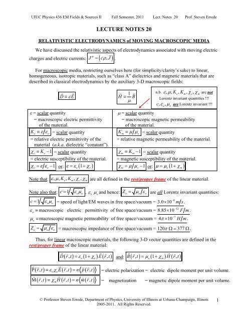
UIUC Physics 436 EM Fields & Sources II Fall Semester, 2011 Lect. Notes 20 Prof. Steven ErredeLECTURE NOTES 20RELATIVISTIC ELECTRODYNAMICS of MOVING MACROSCOPIC MEDIAWe have discussed the relativistic aspects of electrodynamics associated with moving electricμJ = cρ,J .charges and electric currents: ( )For macroscopic media, restricting ourselves here (for simplicity/clarity’s sake) to linear,homogeneous, isotropic materials, such as “class A” dielectrics and magnetic materials that aredescribed in classical electrodynamics by the auxiliary 3-D macroscopic fields: 1 D≡ ε EH ≡ Bμε = scalar quantityμ = scalar quantity= macroscopic electric permittivity = macroscopic magnetic permeabilityof the material.of the material.Ke≡ ε εo = scalar quantity Km ≡ μ μo= scalar quantity= relative electric permittivity of the = relative magnetic permeability of the material.material (a.k.a. dielectric “constant”).χe≡ Ke− 1 = scalar quantity χm≡ Km− 1 = scalar quantity= electric susceptibility of the material. = magnetic susceptibility of the material.χ εε 1 ε = ε 1+ χχ μ μ 1 μ = μ 1+χe= − or: ( )ooem= − or: ( )Note that: ε, μ, K , K , χ , χ are all defined in the rest/proper frame of the linear material.e m e mNote also that: c = 1 εoμo, εoμoand hence: Zo = μo εo are all Lorentz invariant quantities:−8c = ε μ = speed of light/EM waves in free space/vacuum = 3.0× 10 ms.1o oεo≡ macroscopic electric permittivity of free space/vacuum =μo≡ macroscopic magnetic permeability of free space/vacuum =oom−128.85 10 Fm× .π × .−74 10 H mZo = μo εo = macroscopic impedance of free space/vacuum = 120 π Ω 377 Ω .Thus, for linear macroscopic materials, the following 3-D vector quantities are defined in therest/proper frame of the linear material: D r t( , ) = ε ( 1 + χ ) E( r,t) Ρ ≡ = Μ ≡ =( rt , ) εχo eErt ( , ) n prt ( , )( rt , )χ H( rt , ) nmrt ( , )moeand: B ( rt , ) = μ ( 1 + χ ) H( rt , )on.b. ε, μ, Ke, Km, χe,χmare notLorentz invariant quantities !!!c, ε , μ are Lorentz invariant !!!mo= electric polarization = electric dipole moment per unit volume.= magnetization = magnetic dipole moment per unit volume.o© Professor Steven Errede, Department of Physics, University of Illinois at Urbana-Champaign, Illinois2005-2011. All Rights Reserved.1

UIUC Physics 436 EM Fields & Sources II Fall Semester, 2011 Lect. Notes 20 Prof. Steven ErredeThus, we obtain the {usual} constitutive/auxilliary relations for linear media defined in therest/proper frame of the linear material:D ( r, t) = εoE ( r, t) +Ρ ( r,t)and: ( ) 1 H r, t = B( r, t) −Μ( r,t)μIn order to go over to a relativistic formulation of these relations, we must be careful/precisein their physical meaning. In particular, the electric permittivity, ε and magnetic permeability,μ are defined in the rest frame of the material – i.e. ε is the proper electric permittivity and μis the proper magnetic permeability Thus, the macroscopic fields D, Ρ,E and H, Μ,B are all defined in the rest/proper frame ofthe linear material – i.e. they are proper macroscopic electromagnetic fields.Because we already know/understand the Lorentz transformation properties of E and B ,we can write the auxiliary/constitutive relations as:o 1 E r t D r t r tε( )( , ) = ( , ) −Ρ( , )o ( )and: B( rt , ) = μ H( rt , ) +Μ( rt , )oThe relativistic EM field tensorvF μis:Fμv⎛ 0 Ex c Ey c Ezc⎞⎜⎟−Ex c 0 Bz −By≡ ⎜⎟⎜ −Ey c −Bz 0 Bx⎟⎜−Ez c By −Bx0 ⎟⎝⎠and its relativistic dualvG μis:Gμv⎛ 0 Bx By Bz⎞⎜⎟−Bx 0 −Ez c Eyc 1≡ ⎜⎟=ε⎜−By Ez c 0 −Exc⎟2⎜−Bz −Ey c Exc 0 ⎟⎝⎠ vWe construct a rank-2 anti-symmetric tensor D μv(analogous to F μ ) for the D and H fields.vIt describes the (relativistic six-component) “electromagnetic displacement” field, D μ .v{n.b. again, comparing forms in different textbooks, variations for D μ will be found that dependvon the choice/definition of the metric g μ used and conventions r.e. overall constants, etc. !!! }.⎧ 1 ⎫E = ( D−Ρ⎧ 1 ⎫⎪)Taken together, the auxiliary/constitutive relations ε ⎪⎪E→ D⎨ o ⎬ suggest replacing ε⎪⎪ ⎨ o ⎬B= μo( H +Μ)⎪⎪⎩⎭B → μoH⎪⎩ ⎭⎧ 1 2 ⎫⎪E → D=c DHowever, it is a little “cleaner” if we also divide through by μ o, i.e. replace με⎪⎨ o o ⎬.⎪ B→H⎪⎩⎭μvλσFλσ2© Professor Steven Errede, Department of Physics, University of Illinois at Urbana-Champaign, Illinois2005-2011. All Rights Reserved.

UIUC Physics 436 EM Fields & Sources II Fall Semester, 2011 Lect. Notes 20 Prof. Steven ErredeThenvD μbecomes:Dμv⎛ 0 cDx cDy cDz⎞⎜⎟−cDx 0 Hz−Hy≡ ⎜⎟⎜ −cDy −H z0 Hx ⎟⎜−cDz Hy−Hx0 ⎟⎝⎠SI units check:Coul AmpsD= , H =2m mCoul m AmpcD = =2m sec mWe also construct the relativistic dual ofvD μ , which isvH μ(the analog ofvG μ ), defined as:Hμv⎛ 0 Hx Hy Hz⎞⎜⎟−Hx 0 −cDz cDy1≡ ⎜⎟=ε⎜−Hy cDz 0 −cD⎟x 2⎜−Hz −cDy cDx0 ⎟⎝⎠μvλσDλσvThe relativistic dual tensor H μvmay also be obtained directly from D μ by carrying out an appropriate duality transformation on the D and H -fields, analogous to that for the E and B -fields:⎧ E′ = EcosϕD+ cBsinϕD⎫ π⎨⎬ ϕD= − 90 =−⎩cB′ = cB cos ϕD− E sinϕD⎭2⎧cD′ = cD cos ϕD+ H sinϕD⎫ π⎨⎬ ϕ = − 90 =−⎩ H′ = HcosϕD−cDsinϕD⎭2or:or:⎛E′ ⎞ ⎛cosϕD+ sinϕD⎞⎛E⎞⎜ ⎟= ⎜ ⎟⎜ ⎟⎝cB′ ⎠ ⎝−sinϕDcosϕD⎠⎝cB⎠⎛cD′ ⎞ ⎛cosϕD+ sinϕD⎞⎛cD⎞⎜ ⎟= ⎜ ⎟⎜ ⎟⎝H′ ⎠ ⎝−sinϕDcosϕD⎠⎝H⎠Then forϕ D=−90 , we replace: cD →+ H and: H →− cD inDμvμv→ H :Dμv⎛ 0 cDx cDy cDz⎞⎜⎟−cDx 0 Hz−Hy≡ ⎜⎟⎜ −cDy −H z0 Hx ⎟⎜−cDz Hy−Hx0 ⎟⎝⎠⇒Hμv⎛ 0 Hx Hy Hz⎞⎜⎟−Hx 0 −cDz cDy1≡ ⎜⎟=ε⎜−Hy cDz 0 −cD⎟x 2⎜−Hz −cDy cDx0 ⎟⎝⎠μvλσDλσμvLikewise,we may analogously define/construct a rank-2 anti-symmetric tensor Ρ for theΡ and Μ fields describing the (relativistic six-component) electromagnetic “polarization” fieldμvΡ .Since Ρ Coulombshas the same SI units as D ⎛⎜⎞⎟ and Μ Ampshas the same SI units as⎝ meter ⎠H ⎛⎜⎞⎟⎝ meter ⎠we see that:⎛ 0 cΡx cΡy cΡz⎞ Note the minus sign reversal here for⎜⎟−Ρ cx0 −ΜμvzΜ Μyx, Μy,Μzrelative to Ρx, Ρy,Ρzdue toΡ ≡⎜⎟⎜ −Ρ cyΜz 0 −Μx⎟⎜D = εoE +Ρ 1 vs. H = B−M!!!−Ρ cz−Μy Μx0 ⎟μ⎝⎠oF μAgain, we can construct a relativistic dual ofvvand/or H μv, for D μ }, defined as:μvΡ which we callμvΜ {the analog ofvG μ , for© Professor Steven Errede, Department of Physics, University of Illinois at Urbana-Champaign, Illinois2005-2011. All Rights Reserved.3

UIUC Physics 436 EM Fields & Sources II Fall Semester, 2011 Lect. Notes 20 Prof. Steven Errede⎛ 0 −Μx−Μy−Μz ⎞⎜⎟Μx 0 −cΡ vzcΡμy 1 μvλσΜ ≡ ⎜⎟= ε Ρ⎜Μy cΡz 0 −cΡ⎟x 2⎜Μz −cΡy cΡx0 ⎟⎝⎠λσAgain, note the minus sign reversal here forΜx, Μy,Μzrelative to Ρx, Ρy,Ρzdue toD = ε E +Ρ 1 vs. H = B−M!!!oμoμvμvAgain, the relativistic dual tensor Μ can be obtained directly fromΡ by carrying out thesame duality transformation as above, but on the Ρ and Μ fields. Since Ρ has the same SI unitsas D , and Μ has the same SI units as H we see that:⎧−Ρ=−Ρ c ′ c cosϕD+ΜsinϕD⎫ πϕ = −⎨⎬ 90 =−⎩ Μ=+Μ ′ cosϕD+Ρ c sinϕD⎭2or:⎛−cΡ′ ⎞ ⎛cosϕD+ sinϕD⎞⎛−cΡ⎞⎜ ⎟= ⎜ ⎟⎜ ⎟⎝ Μ′⎠ ⎝−sinϕDcosϕD⎠⎝ Μ ⎠Then forϕ D=−90 , we replace: cΡ→−Μ and: Μ →+ cΡ inμvμvΡ →Μ :⎛ 0 cΡx cΡy cΡz⎞⎜⎟−Ρ cx0 −ΜvzΜμyΡ ≡⎜⎟⎜ −Ρ cyΜz 0 −Μx⎟⎜−Ρ cz−Μy Μx0 ⎟⎝⎠⇒⎛ 0 −Μx−Μy−Μz ⎞⎜⎟Μx 0 −cΡ vzcΡμy 1 μvλσΜ ≡ ⎜⎟= ε Ρ⎜Μy cΡz 0 −cΡ⎟x 2⎜Μz −cΡy cΡx0 ⎟⎝⎠λσFrom the classical electrodynamic auxiliary/constitutive relations: 1or: E = ( D−Ρ)εo and: B= μo( H +Μ)in terms of the EM field tensors and their duals are:D1= F +Ρ and:μμv μv μvoHD = εoE +Ρ 1 and: H = B−Μμwe see that their (combined) relativistic equivalents,1= G +Μ n.b. must be + here !!!μμv μv μvμv μv μvv v vor: F = μo( D −Ρ ) and: Gμ = μo( Hμ −Μμ)n.b. If we defineD1≡ F +Ρ then we must have the + sign inμμv μv μvoμv1 μvλσbecause the dual EM field tensor G = ε Fλσ2v v v 1 v 1 vconnects to: G μ = μo( H μ −Μ μ ) = ε μ λσ F μ λσλσ= μoε( Dλσ −Ρλσ ) .2 2o1H = G + Mμμ v μ v μ voo4© Professor Steven Errede, Department of Physics, University of Illinois at Urbana-Champaign, Illinois2005-2011. All Rights Reserved.

UIUC Physics 436 EM Fields & Sources II Fall Semester, 2011 Lect. Notes 20 Prof. Steven ErredeThus the macroscopic relativistic EM field tensors and their duals are:Fμv⎛ 0 Ex c Ey c Ezc⎞⎜⎟−Ex c 0 Bz −By≡ ⎜⎟⎜ −Ey c −Bz 0 Bx⎟⎜−Ez c By −Bx0 ⎟⎝⎠Gμv⎛ 0 Bx By Bz⎞⎜⎟−Bx 0 −Ez c Eyc 1≡ ⎜⎟=ε⎜−By Ez c 0 −Exc⎟2⎜−Bz −Ey c Exc 0 ⎟⎝⎠μvλσFλσDμv⎛ 0 cDx cDy cDz⎞⎜⎟−cDx 0 Hz−Hy≡ ⎜⎟⎜ −cDy −H z0 Hx ⎟⎜−cDz Hy−Hx0 ⎟⎝⎠Hμv⎛ 0 Hx Hy Hz⎞⎜⎟−Hx 0 −cDz cDy1≡ ⎜⎟=ε⎜−Hy cDz 0 −cD⎟x 2⎜−Hz −cDy cDx0 ⎟⎝⎠μvλσDλσ⎛ 0 cΡx cΡy cΡz⎞⎜⎟−Ρ cx0 −ΜvzΜμyΡ ≡⎜⎟⎜ −Ρ cyΜz 0 −Μx⎟⎜−Ρ cz−Μy Μx0 ⎟⎝⎠⎛ 0 −Μx−Μy−Μz ⎞⎜⎟Μx 0 −cΡ vzcΡμy 1 μvλσΜ ≡ ⎜⎟= ε Ρ⎜Μy cΡz 0 −cΡ⎟x 2⎜Μz −cΡy cΡx0 ⎟⎝⎠λσLet us explicitly check the correctness/validity of these relations – assuming things are internallyvcorrect within each of the EM field tensors T μ , then we only need to check two non-zero elements:For the0112T components: For the T components:DcDDD1= F +Ρμ01 01 01xo1 Ex= + cΡμ c01= E +Ρx 2 x xμoc= ε E +Ρx o x xor:D = ε E +ΡoxHH1= G +Μμ01 01 011= B −Μμor: 1 H = B−Μμox x xooDH1= F +Ρμ12 12 121= B −Μμor: 1 H = B−Mμoz z zooH1= G +Μμ12 12 12o1− cD =− E −cΡμ cDDz z zo1= E +Ρz 2 z zμoc= ε E +Ρz o z zor:D = ε E +ΡoThus, we obtain the relativistic auxiliary/constitutive relations and their duals:D1= F +Ρ and:μμv μv μvoH1= G +Μμμ v μ v μ vμv μv μvv v vor: F = μo( D −Ρ ) and: Gμ = μo( Hμ −Μμ)o© Professor Steven Errede, Department of Physics, University of Illinois at Urbana-Champaign, Illinois2005-2011. All Rights Reserved.5

UIUC Physics 436 EM Fields & Sources II Fall Semester, 2011 Lect. Notes 20 Prof. Steven ErredeLorentz Transformations of the Relativistic Macroscopicμ v μF , Dv μ,vG , H , ΜμElectrodynamical Fields { Ρ } and Their Duals { v μ v μ v}We already know/have shown that in the the relativistic EM fields in frame IRF(S') are relatedμvμ v λσμvμ v λσto those in IRF(S) via: F′ =ΛλΛ σFand G′ μv=ΛλΛ σG, where Λ = the Lorentztransformation tensor. For linear macroscopic media, we have linear relations between { DEΡ , , } and also between{ H , B , Μμv 1 μv μvμv 1 μv μv} , which hold relativistically between D = F +Ρ and also H = G +Μ .μμ∴We explicitly see using the Lorentz transformations of individual field quantities defined inμvμ v λσ μvμ v λσμvμ v λσIRF(S) to the frame IRF(S'): D′ =Λ Λ D , F′ =Λ Λ F and: Ρ ′ =Λ Λ Ρλσμv 1 μv μvv⎡ 1 v v⎤That: D = F +Ρ ⇒ Λ μ Dλσ Fμ μλΛ σ ⎢ = +Ρ ⎥μo⎣ μo⎦v 1 v v⇒μ Dλσ μ Fλσ μ λσμv 1 μv μvΛλΛ σ= ΛλΛ σ+ΛλΛ σΡ ⇒ D′ = F′ +Ρ ′ holds in IRF( S′ ).μμoLikewise, for the dual tensors we explicitly see using the Lorentz transformations of individualμvμ v λσ μvμ v λσfield quantities defined in IRF(S) to the frame IRF(S'): H′ =Λ Λ H , G′ =Λ Λ Gand:Μ ′ =Λ Λ Μμvμ v λσλ σμv 1 μv μvv⎡v 1 v v⎤That: H = G +Μ ⇒ Λ μ Hμ Gμ μλΛ σ ⎢ = +Μ ⎥μo⎣ μo⎦v 1 v v⇒μ Hλσ μ Gλσ μ λσμv 1 μv μvΛλΛ σ= ΛλΛ σ+ΛλΛ σΜ ⇒ H′ = G′ +Μ ′ holds in IRF( S′ ).μμoEquivalently, we can alternatively express these as a simple Lorentz transformation of the macroscopic { ED , , Ρ} and { BH , , Μ}fields, e.g. for a Lorentz transformation from the rest/proper frame IRF(S) where the macroscopic { ED , , Ρ} and { BH , , Μ}fields are defined,to another IRF( S′ ) which is moving with velocity v to one of the xˆ, yˆ, or zˆaxes (e.g. v =+ vxˆ).oλσoλoσλλoσσ6© Professor Steven Errede, Department of Physics, University of Illinois at Urbana-Champaign, Illinois2005-2011. All Rights Reserved.

UIUC Physics 436 EM Fields & Sources II Fall Semester, 2011 Lect. Notes 20 Prof. Steven ErredeWe have already shown {in P436 Lecture Notes 19 p. 1-3} that the components ofv transform as:that are || and ⊥ to the boost direction ( )IRF( S′ ): IRF(S): IRF( S′ ): IRF(S):Eand BE′ = E|| ||B′ = B|| ||Thus:⊥⊥ ( ( ) ) ⊥⊥E ( β cB)⊥E′ = γ E + v×B( )= γ + ×1⊥⊥ ⎛ ⊥ B′ ⎞= γ ⎜B −2 ( v×E)⎟⎝ c ⎠⊥⎛⊥⎛ E ⎞ ⎞= γB − ⎜β×⎟⎜ ⎝ c ⎠ ⎟⎝⎠where: γ =121−βand:vβ =c vβ =cIRF( S′ ): IRF(S): IRF( S′ ): IRF(S):D′ = D|| ||⊥ ⎛ 1 ⊥D′ = γ ⎜D + v×H2⎝ c⎛ ⊥ 1 = γ ⎜D+ ×⎝ 2( )( β H)⊥⊥⎞⎟⎠⎞⎟⎠H′ = H|| ||⊥⊥ ( ( ) ) ⊥⊥H c( β D)⊥H′ = γ H − v×D( )= γ − ×And similarly:IRF( S′ ): IRF(S): IRF( S′ ): IRF(S):|| ||Ρ ′ =Ρ⊥ ⎛ ⊥ 1 Ρ ′ = γ ⎜Ρ − ×Μ2⎝ c⎛ ⊥ 1 = γ ⎜Ρ − ×Μ⎝ c( v )( β )⊥⎞⎟⎠⎞⎟⎠⊥|| ||Μ ′ =Μ⊥⊥ ( ( v ) ) ⊥⊥c( β )⊥Μ ′ = γ Μ + ×Ρ( )= γ Μ + ×Ρn.b. note the sign reversals hererelative to the above relations !!!And we also have:In IRF( S′ ): In IRF(S): D′ = εoE′ + P′D = εoE + P1H ′ = B ′ −M ′ H 1 = B−Mμμoon.b. We see from these two relations that in the rest/proper frameIRF(S 0 ) of a polarized dielectric with electric polarization Ρ 0(or a magnetized material with magnetization Μ 0) if the linearmaterial is moving e.g. with velocity v =+ vxˆin the lab frameIRF(S), an observer in the lab frame will “see” a combination ofelectric polarization Ρ and magnetization Μ in both cases!1n.b. εo, μo,c = are all Lorentz invariant quantities.ε μoo© Professor Steven Errede, Department of Physics, University of Illinois at Urbana-Champaign, Illinois2005-2011. All Rights Reserved.7

UIUC Physics 436 EM Fields & Sources II Fall Semester, 2011 Lect. Notes 20 Prof. Steven ErredeRelativistic Invariants Associated with Macroscopic Relativistic EM Fields We have already shown/discussed that for the E and B -field tensorsμvandvF Gμ , there aretwo and only two relativistic Lorentz invariant quantities:1)⎛F F F F G G G G 2 B⎜⎝μv μv μv μv2μv =μv =−μv =−μv= ⎜ −2⎛E⎞ ⎞⎜ ⎟⎝ c ⎠ ⎟⎠μv μv μv μv42) F Gμv = FμvG = G Fμv = GμvF =− ( EiB)c Since the (inner) product of a contravariant tensor of rank-n with any other covariant tensor ofthe same rank-n is a Lorentz invariant quantity (i.e. same/valid in any inertial reference frame,μ v μF , Dv μ,vμ v μG , Hv μ, Μv we can literally have a “fieldwe see that for { Ρ } and their duals { }day” / go wild {!!!} and form many additional Lorentz invariant quantities, such as:2( )v v v v23) D μ D = D D μ =− H μ H =− H H μ = 2 H − ( cD)μv μv μv μvv v v v4) D μ HvDvH μ H μ DvHvD μμ=μ=μ=μ=−4c( DiH)μv μv μv μv25) Ρ Ρ = Ρ Ρ = −Μ Μ = −Μ Μ = 2 Μ − ( Ρ )2( )μv μv μv μv c μv μv μv μv6) Ρ Μμv =ΡμvΜ =Μ Ρμv =ΜμvΡ =+ 4c( ΡΜ i )We can also form the “crossed” Lorentz invariants:See these lecture notes, p.10 for details.7)8)9)F D = F D = D F = D F =− G H =− G H =− H G =− H Gμ v μ v μ v μ v μ v μ v μ v μ vμv μv μv μv μv μv μv μvF Ρ = F Ρ =Ρ F =Ρ F =−G Μ =−G Μ =−Μ G =−Μ Gμ v μ v μ v μ v μ v μ v μ v μ vμv μv μv μv μv μv μv μvD Ρ = D Ρ =Ρ D =Ρ D =−H Μ =−H Μ =−Μ H =−Μ Hμ v μ v μ v μ v μ v μ v μ v μ vμv μv μv μv μv μv μv μvAs well as:10)11)12)F Μ = F Μ =Μ F =Μ F =−G Ρ =−G Ρ =−Ρ G =−Ρ Gμ v μ v μ v μ v μ v μ v μ v μ vμv μv μv μv μv μv μv μvD G = D G = G D = G D =− H F =− H F =− F H =− F Hμ v μ v μ v μ v μ v μ v μ v μ vμv μv μv μv μv μv μv μvD Μ = D Μ =Μ D =Μ D =−H Ρ =−H Ρ =−Ρ H =−Ρ Hμ v μ v μ v μ v μ v μ v μ v μ vμv μv μv μv μv μv μv μvThus, we can form a total of 12 unique bi-linear Lorentz invariant quantities using theμ v μF , D v μ, Pvμ v μG , H v μ, Mv .relativistic macroscopic EM field tensors { } and their duals { }8© Professor Steven Errede, Department of Physics, University of Illinois at Urbana-Champaign, Illinois2005-2011. All Rights Reserved.

UIUC Physics 436 EM Fields & Sources II Fall Semester, 2011 Lect. Notes 20 Prof. Steven ErredeWe explicitly work out the first four of these new Lorentz invariant quantities:3)μv00 00 01 01 02 02 03 03D D =+ vD D − D D − μD D − D D− D D + D D + D D + D D10 10 11 11 12 12 13 13− D D + D D + D D + D D20 20 21 21 22 22 23 23− D D + D D + D D + D D30 30 31 31 32 32 33 33= 0 −cD−cD2 2x2 2 2( H c D )2 2 2 2yz− cD + 0 + H + H2 2 2 2x z y− cD + H 0 + H2 2 2 2y z x− cD + H + H + 02 2 2 2z y x= 2 −− c D4)μv00 00 01 01 02 02 03 03D H =+ vD H − D H − μD H − D H− D H + D H + D H + D H10 10 11 11 12 12 13 13− D H + D H + D H + D H20 20 21 21 22 22 23 23− D H + D H + D H + D H30 30 31 31 32 32 33 332= 0 −cD H −cDH( i )xx− cDHy x z z− cD + 0 + H + H2 2 2 2x z y− cD + H 0 + H2 2 2 2y z x2 2 2 2− cDz + Hy + Hx+ 0 =−4c D H5)μv00 00 01 01 02 02 03 03Ρ Ρμv=+Ρ Ρ −Ρ Ρ −Ρ Ρ −Ρ Ρ−Ρ Ρ +Ρ Ρ +Ρ Ρ +Ρ Ρ10 10 11 11 12 12 13 13−Ρ Ρ +Ρ Ρ +Ρ Ρ +Ρ Ρ20 20 21 21 22 22 23 23−Ρ Ρ +Ρ Ρ +Ρ Ρ +Ρ Ρ30 30 31 31 32 32 33 33= 0 −cΡ −cΡ2 2 2( c )2 2 2 2xy2 2z−cΡ + 0 +Μ +Μ2 2 2 2x z y−cΡ +Μ + 0 +Μ2 2 2 2y z x−cΡ +Μ +Μ + 02 2 2 2z y x= 2 Μ − Ρ− c Ρ© Professor Steven Errede, Department of Physics, University of Illinois at Urbana-Champaign, Illinois2005-2011. All Rights Reserved.9

UIUC Physics 436 EM Fields & Sources II Fall Semester, 2011 Lect. Notes 20 Prof. Steven Errede6)μv00 00 01 01 02 02 03 03Ρ Μμv=+Ρ Μ −Ρ Μ −Ρ Μ −Ρ Μ−Ρ Μ +Ρ Μ +Ρ Μ +Ρ Μ10 10 11 11 12 12 13 13−Ρ Μ +Ρ Μ +Ρ Μ +Ρ Μ20 20 21 21 22 22 23 23−Ρ Μ +Ρ Μ +Ρ Μ +Ρ Μ30 30 31 31 32 32 33 33= 0 +Ρ Μ + Ρ( i )2x xcΜ + cΡ Μy y z z+ cΡ Μ + 0 + cΡ M + cΡ Μx x z z y y+ cΡ Μ + cΡ Μ + 0 + cΡ Μy y z z x x+ cΡzΜ z+ cΡyΜ y+ cΡxΜ x+ 0= + 4cΡ ΜWe can also form “higher-order” tri-linear and quadri-linear invariants from combinations ofμ{ v μ, v μF D , Pvμ} and{ v μ, v μG H , Mv} , e.g.:Fμ vDΡ λ (and all allowed permutations): μvμλ vλσF D Ρ G (and all allowed permutations):μλ vσShorthand:Shorthand:FFF GGG FFG etc. FFFF etc.FFD GGH FFHFFFDFFP GGM FFMFFFPFDD GHHFFFGFDD GHMFFFHFPP GMMFFFMDDD HHHPPP MMM etc.etc.e.g. F D P G H and all allowed permutationse.g. F D P G H M and all allowed permutationsNote: Obviously, not all of these combinations of fields will be truly unique!e.g.and:⎡ ⎛vF F F F ( F Fv)( F F ) B⎢⎜⎣ ⎝μvλσ μ λσ2μvλσ=μ λσ= ⎢2⎜−⎛ E ⎞⎜ ⎟⎝ c ⎠⎛ ⎞Ρ Ρ = Ρ Ρ = − ⋅ Μ − Ρ⎜ ⎜ ⎟⎝ c ⎠ ⎟⎝ ⎠2μvλσ μ λσEF FμvλσF Fμ λσB c2⎞⎤⎟⎥⎠⎥⎦v2 ⎛ ⎞2 2 2( v)( ) 2⎜⎟ 2( )⎛ ⎞= 4B − Μ − Ρ⎜ ⎜ ⎟⎝ c ⎠ ⎟⎝ ⎠22 ⎛E⎞ 2 2 2( c )210© Professor Steven Errede, Department of Physics, University of Illinois at Urbana-Champaign, Illinois2005-2011. All Rights Reserved.

UIUC Physics 436 EM Fields & Sources II Fall Semester, 2011 Lect. Notes 20 Prof. Steven ErredeMaxwell’s Equations in Tensor Notation for Macroscopic Linear MediaThe classical electrodynamics version of Maxwell’s equations for macroscopic linear media are: i 1 1where: ρToT = ρfree + ρboundε ε1.) Gauss’ Law: ∇ E = ρ = ToT ( ρ + freeρbound)ooThe auxiliary/constitutive relation D = εoE +Ρgives: 1 ∇ iE= ρToT⇒ ∇ i D = ρfree and ∇ i P =−ρboundεo D= ε E , Ρ= ε χ Eo e 2.) No magnetic monopoles: ∇ i B = 03.) Faraday’s Law: ∂B∇× E =− ∂ t⇒ ε = ε ( 1+χ ) 1 ∂E4.) Ampere’s Law: ∇× B − = μ2oJc ∂tThe auxiliary/constitutive relationoToTewhere: 1 H = B−Μμo∇ iD = ε ∇ iE +∇ i P J = J + J + JM PToT free bound boundgives:o 1 ∇× H = ∇× B−∇×ΜμEMaxwell’s displacement current term JD= ε ∂o , polarization current:∂t ∂D M∇× H = Jfree+ and ∇× M = J bound where:D E P ∂ ∂ ∂ = ε + = J + J∂ t∂t ∂t ∂topJ boundpo D bound∂Ρ= ∂ t 1 H = B , mμΜ= χ H⇒ μ = μ ( 1+χ )omRelativistically, we have seen that Maxwell’s four equations for free space / the vacuum{i.e. no matter present} are contained within the two tensor relations:∂F∂xμvv= μ JoμToTμv∂Gand: = 0v∂xGiven that:D1= F +Ρ and:μμv μv μvoH1= G +Μμμ v μ v μ vo© Professor Steven Errede, Department of Physics, University of Illinois at Urbana-Champaign, Illinois2005-2011. All Rights Reserved.11

UIUC Physics 436 EM Fields & Sources II Fall Semester, 2011 Lect. Notes 20 Prof. Steven ErredeWe see that the inhomogenous relativistic Maxwell relations are:∂F∂xμvv= μ JoμToT ⎧∇ iD= ρ∂D∂ ∇ − =⎩ ∂tμvfreeμ⎪= Jfree= ( cρfree,Jvfree ) ⎨ x ∂D⎪ iH Jfree μv⎧∇ iP=−ρbound∂Ρμ⎪= Jbound = ( −cρbound , Jv bound ) ⎨ ∂ xP M ∂P ⎪Jbound = Jbound + Jbound= +∇×Μ⎩∂tWhereas the homogenous relativistic Maxwell relations are:⎧ ⎪∇ iH=−∇iΜμv⎧∇ iB= 0μvμv∂G⎪ ∂H ∂M ⎪ 1 ∂H= 0v ⎨ ∂x∂B⇒ =− Dvv ⎨∇× =−2⎪∇× E =− ∂x ∂x ⎪ c ∂t⎩ ∂t⎪ 1 ∂Μ⎪∇×Ρ =+2⎩ c ∂tThe relativistic constitutive relations for linear, homogeneous, uniform, isotropic media {i.e. the relativistic analogs of D= ε E and B = μH} were proposed by H. Minkowski as:μv2 μvμv1 μvD ηv= c εFηvand: H ηv= G ηvμn.b.μThe relativistic EM field tensors are contracted with the proper 4-velocity, η .The relativistic EM field tensors are defined in the rest/proper frame IRF(S) of the linear material.ε is the proper electric permittivity and μ is the proper magnetic permeability.Both quantities are defined in the rest/proper frame IRF(S) of the linear material.μη is the (contravariant) proper 4-velocity of the material.12© Professor Steven Errede, Department of Physics, University of Illinois at Urbana-Champaign, Illinois2005-2011. All Rights Reserved.

UIUC Physics 436 EM Fields & Sources II Fall Semester, 2011 Lect. Notes 20 Prof. Steven ErredeWe can easily show that these formulae give the correct constitutive relations when the linearη = − . Here the sum over v collapses to a single term:material is at rest, i.e. when ( )vc,0,0,0In therest/properframe of thelinear material:η = ε η ⇒μv2 μvDvc Fμv1 μvH ηv= G ηv⇒ HμvD η c εFη= ⇒ − cD =−c 2 ε ( E c)μ0 2 μ00 01 1η = G η ⇒ − H =−μμ0 μ00 0Bμ ⇒ D= ε E⇒ 1 H = BμIf the linear medium is moving e.g. in the lab frame IRF(S) with ordinary velocityu then: μv2 μvμv1 μvηv = ( − γc, γu) = γ ( −c,u). Then for u ≠ 0 : D ηv= c εFηvand: H ηv= G ηvμFor μ = 0 : D η = D η + D η + D η + D η = + cD γu + cD γu + cD γu = γc D u( ) ( ) ( ) ( i )0v00 01 02 03v 0 1 2 30x x y y z z0v 00 01 02 03 E ExEzF ηv = F η0 + F η1+ F η2 + F η3= 0 + γux + γuy + γuz= γ E uc c c c0v2 0v 2 γ∴ D ηv= c εFηv⇒ γc( D u) c ε ⎛ ⎞ i = ⎜ ⎟( Ei u)or: Du i = ε ( Eu i )⎝c⎠And:0v00 01 02 03H ηv = H η0 + H η1+ H η2 + H η3= Hx( γux) + Hy( γuy) + Hz( γuz) = γ ( Hiu)0v00 01 02G η = G η + G η + G η + G3η = B γu + B γu + B γu = γ Biu∴1Gμy1( ) ( ) ( ) ( i )( ) ( ) ( ) ( )v 0 1 2 3 x x y y z z0v0v 1 1 ηv= ηv⇒ γ ( Hu i ) = γ ( Bu i ) or: Hu i = ( Bu i )HSimilarly for μ = 1:μμ( ( ) )x( )1v10 11 12 13 2 2D ηv = D η0 + D η1+ D η2 + D η3=+ γc Dx + γHzuy − γHyuz = γ c Dx+ u× H1v10 11 12 13F η = F η + F η + F η + F η = γE + γB u − γB u = γ E + u× B∴And:v 0 1 2 3 x z y y z x1v2 122 ηv= ε ηv⇒ γx( )xD c F1v10 11 12 130 1 2 3 ( × ) = γ ( x+ ( × ) )cD u H E u B cx( )1 ⇒2 ( )x z y y z xx D+ u× H = ε ⎡E+ ( u×B⎤c⎣ ⎦( ( ) )H η = H η + H η + H η + H η =+ γcH − γcD u + γcD u = γc H − u× D1v10 11 12 13 E Ezy γ 2G η G η0 G η1 G η2 G η3γcBx γ uy γ u ⎡ = + + + =+ − +z= c Bx− ( u×E)⎤c c c ⎣x ⎦1∴ 01 1 v γ 2 1H ηv= G ⇒ γ c( Hx( u D))⎡ − × = c Bx− ( u×E)⎤ 1 ⎡ 1 ⎤⇒ H −μz c ⎣x⎦( u× D) = B− 2 ( u×E)μμ ⎢⎣ c ⎥⎦z© Professor Steven Errede, Department of Physics, University of Illinois at Urbana-Champaign, Illinois2005-2011. All Rights Reserved.13

UIUC Physics 436 EM Fields & Sources II Fall Semester, 2011 Lect. Notes 20 Prof. Steven Erredeμv2 μvμv1 μvThus for: D ηv= c εFηvand: H ηv= G ηvμWe obtain: 1 D2 ( u H) ε ⎡ + × = E+ ( u×B)⎤ 1 ⎡ 1 ⎤c⎣ ⎦ and: H = ( u× D) = B= 2 ( u×E)μ ⎢⎣ c ⎥⎦** 1 1 ⎤μ ⎢⎣ c ⎥⎦ 1 D u H ε ⎡ + × = E+ u×B ⎤2c⎣ ⎦ ⎡ Insert: H = ( u× D) + B= 2 ( u×E)Into: ( ) ( )Solve for D : 1 1 1D + u u D u B u u E E u B2 2 4c × × + c μ× − c μ× × = + ×( ) ( ) ( ) ε ε( ) Use the B ( AC ⋅ ) −C( AB ⋅ ) rule on the first triple cross-product: 1 2 1 1 D+ uuD2 ( i ) =− uD = ε E+ ( u× B) −2 ( u× B) + u× 4 ( u×E)⎡ ⎤ ⎡ ⎤ ⎡ ⎤c ⎣ ⎦ ⎣ ⎦ μc μc⎣ ⎦ But: ( u⋅ D) = ε ( u⋅E)Thus: 2⎛ u ⎞ ε 21− =− + + × − × + −2 2 2 41 1( i ) ε ( ) ( ) ( i )D⎜ ⎟ uuE ⎡E u B⎤ u B ⎡ Euu uE⎤c c ⎣ ⎦ μc μc⎣ ⎦⎝ ⎠2⎧⎪⎡ u ⎤ 1 ⎡ 1 ⎤ ⎡ 1 ⎤⎫⎪= ε ⎨⎢1 − E− 1− 4 2 2 ( E u) u+ ( u× B)1−2 ⎬εμc ⎥c⎢εμc ⎥ i⎢εμc⎥⎩⎪⎣⎦ ⎣ ⎦ ⎣ ⎦⎭⎪Define: γu≡11−uc2 2and:1v ≡ = speed of propagation of EM waves in the linear medium.εμ u v v vD γε ⎧⎛⎞ E ⎛ ⎞ E ⎛ ⎞ ⎤u B E u u⎫ ⎪⎜ ⎟ ⎜ ⎟ ⎜ ⎬c c c⎟⎢⎣ c ⎥⎪⎩⎝ ⎠ ⎝ ⎠ ⎝ ⎠⎦⎪⎭2 2 2 22 ⎪⎡ 1Then: =u ⎨ 1− + 1− + 1− 4 2 2 ( × ) −2 ( i )From equation ** (RHS up above): 1 ⎡ 1 ⎤H = ( u× D) = B= 2 ( u×E)μ ⎢⎣ c ⎥⎦ 1D ε ⎡ = E+ u× B ⎤ − u×H⎣ ⎦ 2cInsert: ( ) ( )Solve for H :14© Professor Steven Errede, Department of Physics, University of Illinois at Urbana-Champaign, Illinois2005-2011. All Rights Reserved.

UIUC Physics 436 EM Fields & Sources II Fall Semester, 2011 Lect. Notes 20 Prof. Steven Errede ⎧ 1 ⎫ 1 ⎡ 1 ⎨ ⎬ ⎤⎩ c⎣ ⎦⎭ μ ⎣⎢ c ⎦⎥ ∴ H u ( u H2 ) ε ⎡E ( u B) ⎤− × − × + + × = B− 2 ( u×E) 1 2 1 1H ⎡ ⎡ 2 ( u H) u u H⎤ ⎤ + − = B− 2 ( u× E) + ε( u× E) + ε ⎡ iu× ( u×B)⎤c ⎣ ⎦ μ ⎢⎣ c ⎥⎦⎣ ⎦ 1 But: ( Hu i ) = ( uH i ) = ( uB i )μ∴ 2⎛ u ⎞ 1 1 ⎡ 1 ⎤ 2H 12 2 ( B u) u B2 ( u E) ε( u E) ε ⎡ ⎜ − ⎟= i + ( B u)u u B⎤c μc μ ⎢− ×c ⎥+ × + i −⎣ ⎦⎝ ⎠⎣⎦1 ⎧ 2 ⎛ 1 ⎞ ⎫= ⎨⎡1− μεu ⎤B+ ⎜εμ− ⎡ 2 ⎟ ( u× E) + ( B u)u ⎤ ⎬μ ⎣ ⎦ i⎩⎝ c ⎠⎣ ⎦⎭But:γu≡11−uc2 2and:v ≡1εμ γ ⎧⎛⎞ ⎛ ⎞ ⎫H B ⎡ ⎪⎜ ⎟ ⎜ u E B u u ⎤ ⎬μ ⎪ v ⎝v c⎟⎣ ⎠⎦⎩⎝⎠⎪⎭2 2u ⎪ u 1 1 ∴ = ⎨ 1− + −2 2 2 ( × ) + ( i ) Thus, the macroscopic D and H -fields in a linear medium moving with ordinary velocity u in IRF(S) in terms of the E and B fields present in IRF(S) are:2 2 22 uv v1D γε ⎧ ⎪ ⎛u1 ⎞ E ⎛ 1⎞ ⎡ ⎤4 2 ( u B) 2 ( E u)u⎫ ⎪= ⎨⎜ − ⎟ + ⎜ − × − ⎬c c⎟⎢i⎣ c ⎥ with:⎪⎩⎝ ⎠ ⎝ ⎠⎦⎪⎭γu≡11−uc2 22 2γ ⎧u ⎪⎛u ⎞ ⎛ 1 1 ⎞ ⎫H 1 B2 2 2⎡ ⎪= ⎨⎜ − ⎟ + ⎜ − ( u× E) + ( Bi u)u ⎤ ⎬μ ⎪ v ⎝v c⎟⎣ ⎠⎦ and:⎩⎝⎠⎪⎭v ≡1εμNote that ε and μ are the proper electric permittivity and the proper magnetic permeability ofthe linear medium – i.e. they are defined in the rest/proper frame of the linear medium.When u = u c, then γ 1 {i.e. the non-relativistic limit}.Thus, keeping only up to terms linear in u :2 ( 1 ( ) )( )D ε E + − v c u× B ≈εEu 1 1 1 1 H B+ − u× E ≈ Bμ ⎝vc ⎠ μ⎛ ⎞ and: ⎜ 2 2 ⎟( )Usually very smallUsually very small© Professor Steven Errede, Department of Physics, University of Illinois at Urbana-Champaign, Illinois2005-2011. All Rights Reserved.15