Lecture Notes 14 - University of Illinois High Energy Physics

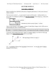
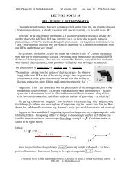
UIUC Physics 435 EM Fields & Sources I Fall Semester, 2007 Lecture Notes 14 Prof. Steven ErredeLECTURE NOTES 14THE MACROSCOPIC MAGNETIC FIELD ASSOCIATED WITH THE RELATIVEMOTION OF AN ELECTRICALLY-CHARGED POINT-LIKE PARTICLEAn electrically charged point-like particle of charge +q (> 0) moving in the lab frame withrelative velocity v (with respect to a fixed coordinate system, origin ϑ ) generates an apparentsolenoidal magnetic field B in the lab reference frame ( cf with particle’s own reference frame:B = 0 there!)For the non-relativistic case (i.e. for v 0: ( ) =+ ( ) ˆqqˆxϕ Bqr Bqr ϕB r = B r − ˆ ϕ =−B r ˆ ϕFor +q > 0: ( ) =+ ( ) ˆFor –q < 0: ( ) ( )( ) ( )q q qˆrv = vzˆ,zˆŷout of pageThe macroscopic B -field associated with a moving electrically charged particle is a solenoidal B r = B r ϕ !field, i.e. ( ) ( ) ˆqq© Professor Steven Errede, Department of Physics, University of Illinois at Urbana-Champaign, Illinois2005-2008. All Rights Reserved.1

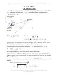
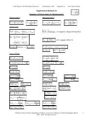
UIUC Physics 435 EM Fields & Sources I Fall Semester, 2007 Lecture Notes 14 Prof. Steven Errede Take cross-products e.g. v × r1 and v × r2 to determine the direction of B-field at observation/fieldP r and P( r 2 ), as shown in the figure below: B ( 2) ( 2)ˆqr =−Bqr yLocal Origin, ϑr 2Observationˆx ẑ r2Point P( r 2 )r 1r′v × r2r1q = r − r′ r1 1 ŷ r2= r2− r′ v × r1Observationv = vzˆ B r =+ B r ypoints ( ) 1Point ( ) 1P r ( ) ( )qˆ1 q 1⎛ μo⎞⎛ ˆ r ⎞ ⎛ μo⎞⎛ r ⎞( ) = N⎜ ⎟⎜ × = ×2 ⎟ ⎜ ⎟⎜ 3 ⎟ ( =Amp − m) Bqr qv qv Teslas⎝4π⎠⎝ r ⎠ ⎝4π⎠⎝ r ⎠This is the magnetic field observed in the lab frame due to a point-like particle with electriccharge q moving with relative velocity v

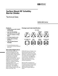
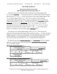
UIUC Physics 435 EM Fields & Sources I Fall Semester, 2007 Lecture Notes 14 Prof. Steven Errede= = r − r ′ = r − r ′ =At the distance of closest approach (t = 0): r rminrmin= minimum.Local Origin, ϑ ẑ r′ˆxŷqv = vzˆSource point S( r′ )r r = r − r′ (lies in x-z plane {here})obs sourcepoint pointObservation/field point P( r )(lies in x-z plane {here})μoqv μoqvB ( , 0) ˆ ˆqrt= = ϕ = yat the distance of closest approach (t = 0).2 24πr 4πr Note the similarity between Eqand Bq-fields of a point-like electrically charged particle: ⎛ 1 ⎞⎛qˆ r ⎞ ⎛ 1 ⎞⎛qr⎞ Eq( r) = ⎜ ⎟⎜ =2 ⎟ ⎜ ⎟⎜ 3 ⎟ Both Eqand Bq-fields decrease as21 r from point⎝4πεo ⎠⎝ r ⎠ ⎝4πεo ⎠⎝ r ⎠ ⎛ μo⎞⎛qv× ˆ r ⎞ ⎛ μo⎞⎛qv× r ⎞2Bq( r) = ⎜ ⎟⎜ =2 ⎟ ⎜ ⎟⎜ 3 ⎟ charge, due to 1 r flux law of virtual photons!!!⎝4π⎠⎝ r ⎠ ⎝4π⎠⎝ r ⎠The Macroscopic Magnetic Field B(r) due to a Steady Current I Flowing in an InfinitelyLong Filamentary WireThe principle of linear superposition tells us that we can view the macroscopic magnetic fielddue to a steady current I flowing in a long filamentary wire as the linear superposition ofmagnetic field contributions associated with each of the individual electric charges q flowing inthe filamentary wire that microscopically constitute/make up the macroscopic steady current I:NNˆi( to)B I ( r ⎛ μ ⎞ ⎛ ⎞, t) = ∑Bq( r , t)= qvi ⎜ ⎟ × ∑r2i= 1 ⎝4π⎠⎜i=1 i () t ⎟⎝ r ⎠Where we have assumed (here) that all charge carriers have the same electric charge q and movealong the filamentary wire with the same velocity v = vzˆ.In the limit that the number of electric charges that are microscopically involved in making upthe macroscopic current I becomes so large that the spacing between adjacent charge carriersbecomes extremely small, e.g. that of atomic dimensions, ~ O(10) Angstroms = 1 nm, then if weare only interested in the net/total macroscopic magnetic field associated with macroscopicdistance scales, e.g. r ~1μm(and larger), then we can safely replace the summation in the aboveexpression by an integral over a continuum of infinitesimal electric charge contributions dq allmoving along the filamentary wire with velocity v = vzˆ.For steady macroscopic currents I ≠ fcn ( t)the time dependence drops out/vanishes in the24N ~ Ο 10 total charge carriers, then the fluctuations aremicroscopic averaging process! Ifq ( )( 12−12σN= Nq~ Ο 10 ), thus fractional fluctuations σNNq 1 Nq~ ( 10 )qq= Ο - negligible!!!© Professor Steven Errede, Department of Physics, University of Illinois at Urbana-Champaign, Illinois2005-2008. All Rights Reserved.3

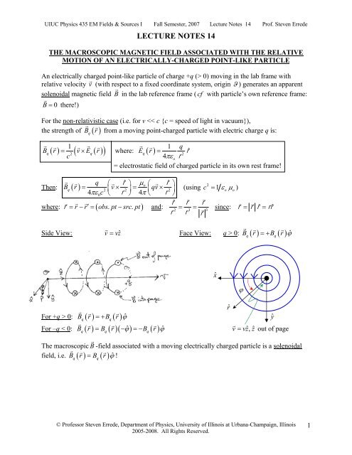
UIUC Physics 435 EM Fields & Sources I Fall Semester, 2007 Lecture Notes 14 Prof. Steven ErredeThus for a macroscopic, steady electric current I flowing in a long (one-dimensional) dB r due to afilamentary wire (of infinitesimal thickness), the infinitesimal contribution ( )macroscopic current I = λfreev= dqv/d flowing in an infinitesimal length d of currentcarryingfilamentary wire with associated infinitesimal source charge increment dq = Id / v is: ⎛ μo⎞ ⎛ r ⎞ dB ( r ) = ⎜ ⎟I ⎜d ( r′) ×3 ⎟ where r = r − r′⎝ 4π⎠ ⎝ r ⎠Connection:Source Point ( )S( r′ )I =qv ⇒ Id = dqvId = Id (since I d )d = vdt d r′dq = λd= λvdtλ line charge (Coulombs/m) r = r −r′I = dq dt = λv B( r )Id = λdv = dqv I , v,d ( r′ ) r′r Local Origin, ϑ P( r ) , Observation/field Point d r′P r n.b. figure drawn for ( ) contribution closest to observation/field point ( ) b ⎛ μ ⎞ bd( r′ ) × r ⎛ μ bd ( r ) ˆo ⎞ ′ × rB r = ∫ dB r = I =3 Ia⎜ ⎟ 24π∫a ⎜ ⎟n.b. assumed4π∫a⎝ ⎠ r ⎝ ⎠ roThen: ( ) ( ) to be constanteverywhere n.b. If I ≠ constant everywhere, I ( r′ ) d=I( r′) dI ( r′ )I ( r′ ) , d ( r′ )Source Point, S( r′ )bI ( r′ ) = r − r′r′ then I must remain inside the integral!a r B( r )ẑ P( r ) Observation/field pointˆx ϑ ŷIn general this integral can often be difficult to perform analytically, but it can be easy to do oncomputer, e.g. using numerical integration techniques!r 4© Professor Steven Errede, Department of Physics, University of Illinois at Urbana-Champaign, Illinois2005-2008. All Rights Reserved.

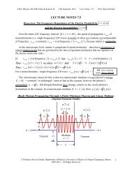
UIUC Physics 435 EM Fields & Sources I Fall Semester, 2007 Lecture Notes 14 Prof. Steven Errede ⎛ μ b ( ) bo ⎞ ⎛I r′ × r ⎞ ⎛ μo⎞ ⎛I( r′) d×r ⎞ I ( r′ ) d=I( r′) d B( r)= ⎜ ⎟ d =3 34π∫a ⎜ ⎟ ⎜ ⎟4π∫a⎝ ⎠ ⎝ ⎠ ⎜ ⎟r = r −r′⎝ r ⎠ ⎝ r ⎠@ Source point, r′ ⎛ μ bo ⎞ ⎛d( r′ ) × r ⎞If I( r′ ) = constant everywhere, this expression simplifies to: B( r)= ⎜ ⎟I34π∫a⎝ ⎠ ⎜ ⎟⎝ r ⎠Griffiths Example 5.5 - The Macroscopic Magnetic Field Due to a Steady Current Flowingin an Infinitely Long Wire: Find the magnetic field B( r )a perpendicular distance r away from an infinitely long straightfilamentary wire carrying a steady / constant / uniform current I. ⎛ μ d ( r ) d ( r ) ˆo ⎞ +∞ ⎛ ′ × r ⎞ ⎛ μ +∞o ⎞ ⎛ ′ × r ⎞ˆx B( r)= ⎜ ⎟I = I3 24π∫−∞⎜ ⎟ ⎜ ⎟4π∫−∞⎝ ⎠ ⎝ ⎠ ⎜ ⎟⎝ r ⎠ ⎝ r ⎠Observation / P( r )Field Point (in x-z plane) θ r = r −r′r 2 2 2r = r +r = r r = r = r + 2 2Local origin ϑ( ŷ out of page) r′r′ = For this problem, which way does ( )βα d r′ zˆ,I = Izˆ( )Source Point S( r′ ) d r′ × r point? Note that: d( r′ ) = d ( r′)ˆ z and that r lies in the x-z plane. By the right-hand rule, the cross product: d× r = dzˆ× ( r ˆ ˆ) ( ˆ ˆ) ( ˆ ˆ)ˆxx+ rzz = rxd z× x + rzd z× z = rxdy = y= 0 Thus, d( r′ ) × r = r ˆxdypoints in the ŷ direction (i.e. out of the page) here, because the fieldpoint P( r )(as drawn above) lies in the x-z plane. However as mentioned earlier, d( r′ ) × ractually points in the ˆϕ -direction (n.b. ˆ ϕ = yˆ when ϕ = 0 ). What is the magnitude of d( r′ ) × ˆ dr d αr ? From the definition of this cross product, dr′ and ˆ r .( ′) × ˆ r ≡ sinwhere α = opening angle between ( )© Professor Steven Errede, Department of Physics, University of Illinois at Urbana-Champaign, Illinois2005-2008. All Rights Reserved.5

UIUC Physics 435 EM Fields & Sources I Fall Semester, 2007 Lecture Notes 14 Prof. Steven ErredeππGeometrically: α = π − β and also: π = θ + β + , hence β = − θ22π π∴ α = π − β = π − + θ = + θ , thus:2 2= 0⎛π ⎞ ⎛π ⎞ ⎛π⎞sinα = sin ⎜ + θ⎟= sin ⎜ ⎟cosθ+ cos⎜ ⎟ sin cos⎝ 2 ⎠ ⎝ 2⎠ ⎝ 2⎠ θ = θ∴ d × ˆ r = d sinαϕˆ = d cosθϕˆrFrom the above figure, note that: cosθ = (or equivalently: r = r cosθ)r( )Then: ( )d r ⎛ μ ⎞ˆB ro +∞⎛ ′ × r ⎞2 2 2 = ⎜ ⎟I24π∫with: r = r + and:−∞⎝ ⎠ ⎜ ⎟( ) ˆ⎛ r ⎞d r′ × ˆ r = dcosθϕ= d⎜ ⎟ ˆ ϕ⎝ r ⎠⎝ r ⎠⎛ ⎞ ⎛ μo⎞ +∞ doI rThen: B( r)Ir⎜ ⎟ μˆ⎛ ⎞ μoI= ⎜ ⎟ ϕ 24π∫=−∞2 2( ) 3 ⎜ ⎟ ˆ ϕ = ˆ ϕ⎝ ⎠ ⎜22r + ⎟ ⎝4π⎠⎝r 2πr⎠ ⎛ μo⎞IB( r) = ⎜ ⎟ ˆ ϕ for an infinitely long filamentary wire carrying a steady current I.⎝2π⎠rAn alternative derivation of this result:∞Since r = r cosθ, we can equivalently express ∫ d in terms of an integral over θ :dsinα= d cosθbut note that: = r tanθ(or equivalently: tanθ = )r1 cosθNote also that: r = r cos θ ⇒ =r rrd = dθ is the Jacobian of the transformation from d → dθ2cos θππNow when =+∞ , θ = and when = −∞ , θ = −22Then:2 r dcosθπ 2 ⎛ μ d ( r ) ˆo ⎞ +∞ ⎛ ′ × r ⎞ ⎛ μo⎞ + ⎛cosθ ⎞⎛r ⎞2B( r)= ⎜ ⎟I = I2 24π∫−∞⎜ ⎟ ⎜ ⎟ π ⎜ ⎟⎝ ⎠ ⎝ r ⎠ ⎝4π∫ ⎜−2 ⎟cosθdθϕˆ⎠ 2 ⎝ r ⎠⎝cosθ ⎠ππ⎛ μo⎞ + cos2⎛θdθ ⎞ ⎛ μo⎞I+ˆ2= ⎜ ⎟Icos d ˆπ ϕ π θ θϕ4π∫ ⎜ ⎟ = ⎜ ⎟−2r 4πr∫−⎝ ⎠ ⎝ ⎠ ⎝ ⎠ 2⎛ μo ⎞I ⎡ ⎛π⎞ ⎛ π ⎞⎤⎛ μo ⎞I ⎛ μo⎞I= ⎜ sin sin ˆ ϕ [ 1 1]ˆ ϕ 2 ˆ ϕ4π ⎟r⎢ ⎜ ⎟− ⎜− ⎟ = −− =2 2⎥ ⎜4π ⎟ ⎜r 4π⎟⎝ ⎠ ⎣ ⎝ ⎠ ⎝ ⎠⎦⎝ ⎠ ⎝ ⎠r o∴ B( r) ˆ−∞⎛ μ ⎞I= ⎜ ⎟ ϕ for an infinitely long filamentary wire carrying steady current I.⎝2π⎠r falls off as 1 r where r = ⊥ distance from the infinitely long wire.Note that B( r )16© Professor Steven Errede, Department of Physics, University of Illinois at Urbana-Champaign, Illinois2005-2008. All Rights Reserved.

UIUC Physics 435 EM Fields & Sources I Fall Semester, 2007 Lecture Notes 14 Prof. Steven ErredeThe Macroscopic Magnetic Field due to a Steady Current Flowing in a Finite Length Wire:What is the B -field associated with a steady current I flowing down a finite length filamentarywire (of length )? Same configuration/geometry as before/above for infinite length wire.( )⎛ μ ⎞I dˆ ϕ ⎛ μ ⎞I⎝4π⎠r⎝4π⎠r2 θ2ooBfiniter = ⎜ ⎟ ∫ = cos d⎜ ⎟ ∫wire1 θ12 2( r + ) ⎛ μo⎞IB ( ) ( sin2sin1)ˆfiniter = ⎜ ⎟ θ − θ ϕwire ⎝4π⎠r1 2Where: sin θ1 = , sinθ2=r + r + 2 2 2 21 2θ θϕˆP( r )r θ1θ2 2rr1Iϑ 12= 2 −1ẑFall ’06 P435 Student – Michael Wiczer made plots of the magnitude of the B-field along finitelength wire for 5 different choices of current:M. Wiczer’s contour plot of magnitude of B-field for steady current I flowing down finite-lengthwire:© Professor Steven Errede, Department of Physics, University of Illinois at Urbana-Champaign, Illinois2005-2008. All Rights Reserved.7

UIUC Physics 435 EM Fields & Sources I Fall Semester, 2007 Lecture Notes 14 Prof. Steven ErredeGriffiths Example 5.6 - The Macroscopic Magnetic Field Due to Circular Steady CurrentOn the Symmetry Axis of a Current Loop:A circular filamentary current loop of radius R lies in x-y plane, with a steady current Icirculating anti-clockwise (viewed from above), as shown in the figure below:IẑObservation/Field PointP r = P z( ) ( )z r r = r − r′RLocal Origin,ϑϕ r′Iŷˆx ⎛ μ d ( r ) ˆo ⎞ ′ ×Bloop( r)= ⎜ ⎟ I24π∫ rC⎝ ⎠ ror: ( ) d( r′ )Source Point S( r′ )(lies in x-y plane) Bloopr = ⎜ ⎟ I ⎛ μ do ⎞ ( r′ ) ×34π∫ C⎝ ⎠ rrWhat is ( ) d r′ × r for this particular problem?By the arc-length formula S Rθ ,and: dr Rd x y( ′) = ( ϕ ) sinϕ( − ˆ)+ cosϕˆ= Rdϕ ( − sin ϕxˆ+ cosϕyˆ) d = d r = Rdϕ= the infinitesimal segment of current loop ( ′)( ) and: r ≡r − r′ = z −r′since r = z = zzˆ r = z − r ′ = zzˆ − R cosϕxˆ+sinϕyˆ∴ ( )ϑRdϕR dr′( )⇐ can see this easily e.g. when ϕ = 0 andand r′ = R( cosϕxˆ+sinϕyˆ)πϕ =28© Professor Steven Errede, Department of Physics, University of Illinois at Urbana-Champaign, Illinois2005-2008. All Rights Reserved.

UIUC Physics 435 EM Fields & Sources I Fall Semester, 2007 Lecture Notes 14 Prof. Steven ErredeThus: ( d( r′ ) × r ) = d( r′ ) × ( r − r′ ) = d( r′ ) × ( z− r′ ) = d( r′) × zzˆ − R( cosϕxˆ+sinϕyˆ)= Rdϕ( − sinϕxˆ+ cosϕyˆ) × zzˆ− R ( cosϕxˆ+sinϕyˆ)( )( )Now:xˆ× yˆ =+ zˆ yˆ× xˆ =− zˆ xˆ× xˆ= 0yˆ× zˆ =+ xˆ zˆ× yˆ =− xˆ yˆ× yˆ= 0zˆ× xˆ =+ yˆ xˆ× zˆ=− yˆzˆ× zˆ=0⇐ Very useful table…Thus:Finally: ⎧ ⎪( d( r′ ) × r ) = Rdϕ⎨− zsinϕ( xˆ× zˆ) + zcosϕ( yˆ×zˆ) ⎪⎩=− yˆ=+ xˆ( ˆ ˆ)+ Rsinϕcosϕx×x= 0( ˆ ˆ)2− R cos ϕ y×x=−zˆ⎫2⎪+ Rsin ϕ( xˆ× yˆ) − Rsinϕcosϕ( yˆ×yˆ)⎬=+ zˆ = 0⎪⎭2 2( d( r′ ) × r ) = Rdϕ { + zsinϕyˆ+ zcosϕxˆ+ Rcos ϕzˆ+Rsinϕzˆ}2 2{ sin ˆ cos ˆ ⎡cos sin ⎤ ˆ}= Rdϕ + z ϕy+ z ϕx+ R⎣ϕ+ϕ⎦z{ sin ˆ cos ˆ ˆ}= Rdϕ + z ϕy + z ϕx + Rz d r′ × = Rd z x+ y + Rz( ( ) r ) ϕ ( cosϕ sinϕ){ ˆ ˆ ˆ}Now:′2 2r = r = r − r = z + R and= +2 2 2r z R and also r3 = ( z2 + R2 ) 3 2Then: ⎛ μ ( ) 2 ( cos sin )o ⎞ dr′ × r ⎛ μ Rd z x y Rzo ⎞ π ϕ ϕ ϕBloop( r)= ⎜ I = I34π⎟ ∫C⎜4π⎟ ∫0 ⎝ ⎠ r ⎝ ⎠ 2 2 2+{ ˆ+ ˆ + ˆ}3( z R )2⎛ μ2 2 2o ⎞ Rzπ π ⎛ μ ⎞ IRπ= I ⎡ ϕdϕxˆ ϕdϕyˆ⎤⎜ dϕzˆ4π⎟ + +0 0⎜4⎟0⎝ ⎠ ⎝ ⎠ocos sin3 32 2 2⎢2 2 2( z R⎣∫ ∫ ⎥⎦π ∫+ ) ( z + R )n.b each of these 2 terms will individually vanish / cancelwhen integrated over all ϕ - i.e. from 0≤ ϕ ≤ 2π!! μ0oRz== 0⎛ ⎞2πloop ( ) = ⎜ ⎟+ sinϕ3 ⎢ ˆ0x − cos2 2 2B r I⎝4π⎠ +( z R )⎡ 22oIRϕ yˆ⎤ π μ⎥+ 2π⎛ ⎜ ⎞⎟⎣ ⎦ ⎝4π⎠ z + R( )0 32 2 2zˆ© Professor Steven Errede, Department of Physics, University of Illinois at Urbana-Champaign, Illinois2005-2008. All Rights Reserved.9

UIUC Physics 435 EM Fields & Sources I Fall Semester, 2007 Lecture Notes 14 Prof. Steven ErredeFinally:2 ⎛μo⎞ RB ( )ˆloopr = ⎜ ⎟ I z3⎝ 2 ⎠ 2 2 2( z + R )The B -field on symmetry axis of a steady current-carrying loop of radius R points in ẑ direction3Note also that B ( ˆloopr = zz)falls off as ∼ 1 z just as a magnetic dipole field should!!i.e. B ( ˆloopr = zz)is the on-axis B -field of a physical (i.e. spatially-extended) magnetic dipole!⇒ A loop carrying a current I generates a magnetic dipole field!!! B ( r )The B -field due to a current loop, on the symmetry ( ẑ)-axis of the loop: “3-D” Side View: ẑ B, nA ˆ,≡ Anˆ at I z B ( r )plane of pageAIRatplane of pageCurrent I coming out of page hereA2= π R = cross-sectional areaof current loopCurrent I going into page hereNote that at the observation point r = zzˆ,the “normal” components of B (i.e. those ⊥ to theẑ -axis) cancel, whereas the “parallel” components of B (i.e. those || to the ẑ -axis) add!The vector area of the current-carrying loop is A=Anˆ(where ˆn is defined by right-hand ruleassociated with direction of current circulation).The Magnetic Dipole Moment of a Current-Carrying Loop of Cross-Sectional Area A The magnetic dipole moment is defined as: m≡ IA( = π R 2Izˆhere) (SI units: Ampere-meters 2 )The vector area of the loop is: A R 2 2= π nˆ( nˆ = zˆhere), the scalar area of the loop: = π RloopThe Magnetic Field on the Symmetry Axis of an N-Turn Current-Carrying Loop:Instead of a single current-carrying loop, what would be the B -field associated with N turns(of very fine wire) for the planar current-carrying loop?Using the principle of linear superposition: ITOT= NI .Aloop10© Professor Steven Errede, Department of Physics, University of Illinois at Urbana-Champaign, Illinois2005-2008. All Rights Reserved.

UIUC Physics 435 EM Fields & Sources I Fall Semester, 2007 Lecture Notes 14 Prof. Steven ErredeThus on the symmetry axis of an N-turn planar loop of radius R carrying a steady current I:⎛2⎞21 R 1 RBturn loop ( ) 1-turn loop ( )ˆˆN−z = NB z = N⎜μoI z⎟=μ3 oNI z3of radius Rof radius R2 2 2 2 22 2⎜2( z R ) ⎟⎝+⎠ ( z + R )The superposition principle also works for / is valid for magnetic phenomena since it isintimately connected to electric phenomena via common / same microscopic physics!The Macroscopic Magnetic Fields Associated with Line, Surface and Volume Currents:For line, surface and volume currents, we summarize their corresponding magnetic fields below: ⎛ μ ( ) ˆ( ) ˆo ⎞ Id ′ r′ × r ⎛ μ I ro ⎞ ′ × rLine Currents: Bline( r)= ⎜ ⎟ =d ′2 24C4Ccurrent π ∫ ′⎜ ⎟π ∫′⎝ ⎠ r ⎝ ⎠ r ⎛ μ ( ) ˆo ⎞ K r′ ×Surface Currents: Bsurface( r)= ⎜ ⎟dA′24Scurrent π ∫ r where r = r − r′ , and r = r = r −r′′⎝ ⎠ r ⎛ μ ( ) ˆo ⎞ J r′ ×Volume Currents: Bvolume( r)= ⎜ ⎟ dτ′24vcurrent π ∫ r and ˆ r = r r = r −r′ r −r′′⎝ ⎠ rn.b. The primed variables denotes integration over the relevant source current distributions.© Professor Steven Errede, Department of Physics, University of Illinois at Urbana-Champaign, Illinois2005-2008. All Rights Reserved.11

UIUC Physics 435 EM Fields & Sources I Fall Semester, 2007 Lecture Notes 14 Prof. Steven ErredeThe Biot-Savart Law:The Calculation of Forces on Current-Carrying Conductors Due to Other Current-Carrying ConductorsWe have previously derived (in P435 Lecture Notes 13) that the net macroscopic magneticforce F mon a current-carrying wire immersed in an external magnetic field B ( r′ ) was:If I = I( r′ )F dF r = = I d r × B r iff I = constant/steady/uniform current!∫( ′) ( ′) ( ′)mCmCext∫is not constant/steady/uniform in space, then more generally: F = I r′ × B r′dm∫C( ) ( )extNow let us consider what F mwould be if Bext( r′ ) is due to a 2 nd current-carrying loop.For simplicity’s sake, we will assume that all currents involved are steady currents.Two Amperian Current Loops: Loop #2:Loop #1: dF ( r′ ) = I d ( r′ ) × B ( r′)m1 1 1extextC 1I 1 d ( r′ )Local r′Origin,ϑI 1 r12= r′ − r′′1C 1 I 2r′′C 2d1( r′′ )I 2C 2The infinitesimal force dFm 1( r′ ) acting on a line segment d1 ( r′ ) macroscopic magnetic field B ( r′ ) at the point r′flowing in loop #2.ext on loop #1 is due to the net that is created by the steady current I2Thus: dFm( r′ ) = I d ( r′ ) × Bext( r′) = infinitesimal force acting on line segment d( r′ )1 1 1of loop #1 due to net B -field from second current loop #2Then the net force on the original steady current-carrying loop (loop #1) is:F dF ( r ) I d m ( r ) B ( r = )1 ∫′ ′ ′Cm=11∫1×ext1 C1= magnetic field at source point r′ (on loop #1) at d r′ due to 2 nd current I 2 flowing in loop #21( )112© Professor Steven Errede, Department of Physics, University of Illinois at Urbana-Champaign, Illinois2005-2008. All Rights Reserved.

UIUC Physics 435 EM Fields & Sources I Fall Semester, 2007 Lecture Notes 14 Prof. Steven ErredeWhat is the net, macroscopic B -field at the point r′ arising from the steady current I2 flowing inthe second current loop #2? It is: ⎛ μo⎞ d2 ( r′′ ) × r12 Bext( r′ ) = ⎜ I2 34π⎟ ∫C where r12≡( r′ −r′′) and r12= r′ −r′′2⎝ ⎠ r12Then: Fm = ( ) ( ) ( )1 ∫dFm r′ =C 1 ∫I1d1r′ × Bextr′1 C1 ⎡ ⎛ μo⎞ d2 ( r′′ ) × r ⎤12= ∫Id11( r′) ×⎢ IC⎜ 2 31 4π⎟ ∫⎥C2⎢⎣⎝⎠ r12 ⎥⎦⎛ μ⎡ do ⎞ 2 ( r′′ ) × r ⎤12= ⎜ ⎟II 1 2d1( r′) ×⎢3⎥4π∫C ∫1 C2⎝ ⎠ ⎢⎣r12 ⎥⎦Or:Fm1⎛ μo⎞= ⎜ ⎟ I I4π ∫ ∫⎝ ⎠ d( r′ ) ×d ( r′′) ×1 2C31 C2r12( r )1 2 12 Now, Newton’s 3 rd Law of Motion holds here, i.e. that: F2→1=−F1 →2 ⎛ μ2( ) ( 1 ( ) 21)o ⎞ dr′′ × dr′× rThus: Fm= I2 ⎜ ⎟ 2I1 34π∫C∫2 C1⎝ ⎠ r≡ − =− − ≡−where ( r′′ r′ ) ( r′ r′′)21⇐ Biot-Savart Law= r ′′ − r ′ = r ′ − r ′′ =r21r12and r21r12 This relation can be / is easily obtained by permuting indices 1 2 and r′ r′′Explicit proof - Use the vector triple cross-product identity: A× B× C = B( AiC) −C( AiB) Expand out the integral for F m 2: d2 ( r′′ ) × ( d1 ( r′ ) × r21) d1 ( r′ ) d2 ( r′′ ) ir 21r21d2 r′′ id1r′∫ = −C ∫ 3 3 32 C ∫ 1 C ∫ 2 C ∫ 1 C ∫2 C1r21r21r21Why does∫ ∫C2 C1 d r d r i( r )( ′) ( ′′)1 2 21 3r21= 0???( ) ( ( ) ( ))C2 C 31 C 3 131 C2 C1 C2r21r ⎢21r21= 0 !!!Why? d1 ( r )( d2 ( r ) 21) d1 ( r )( d2 ( r ) 21)⎡ ′ ′′ ir ′ ′′ ir ( d2 ( r′′) ir21 ) ⎤ = = d( r′) ⎢⎥⎥⎣ ⎦∫ ∫ ∫ ∫ ∫ ∫n.b. Switched orderof integrationThis integral is carried outonly over closed contour C2of loop #2© Professor Steven Errede, Department of Physics, University of Illinois at Urbana-Champaign, Illinois2005-2008. All Rights Reserved.13

UIUC Physics 435 EM Fields & Sources I Fall Semester, 2007 Lecture Notes 14 Prof. Steven ErredeNow: i i =3 2rr ( d ( r′′ ) r ) d ( r′′)( ˆ r )2 21 2 2121 21since r21= r21r21ˆBut what is d2 ( r′′ ) ir ˆ21?? d2 ( r′′ ) i ˆ r21= d2cosθwhere θ = opening between d ( r′′ ) d ( r′′ ) i ˆ r = d cosθ= d( r′′ ) cosθ≡ dr ( r′′ ) = dr( r′′)2 21 2 2 21 21r d r ≡ d cosθ212 21 and ˆ r2 21θd2( r′′ )∴d r d r = rr( 2 ( ′′)i ˆ r21)212 221 21Then:d r ir d r ir d r ( ( ′′)) ( ′′)( ˆ )∫ ∫ ∫2 21 2 2121C =3 2 22 C =2 C2r21r21r21d rBut we know that ∫ 0C 2 ≡ around an (arbitrary) closed loop/contour C !!!re.g. Δ q d rˆq drV = Eq( r) d = i∫ i 0C 2 24πε∫C 4Cor πε ∫or=Thus finally: ⎛ μ21 ( 2 ( ) 1 ( ))o ⎞dr′′ idr′Fm=− I2 ⎜ ⎟ 2I1 34π∫C∫r2 C1⎝ ⎠ r21But:21≡( r ′′ − r ′) =−( r ′ −r r ′′)≡−r12And:21= r ′′ − r ′ = r ′ − r r ′′ = r12∴ Fm= −F2 m1 And: AB i = BA i ⎛ μ12 ( 1 ( ) 2 ( ))o ⎞dr′ idr′′Thus: Fm=− I1 ⎜ ⎟ 1I2 34π ∫C∫r1 CQ.E.D.2⎝ ⎠ r for a point electric charge!!!1214© Professor Steven Errede, Department of Physics, University of Illinois at Urbana-Champaign, Illinois2005-2008. All Rights Reserved.

UIUC Physics 435 EM Fields & Sources I Fall Semester, 2007 Lecture Notes 14 Prof. Steven ErredeExamples of the Use of the Biot-Savart Force Law:The Net Force Between Two Infinitely Long, Parallel Wires Carrying Steady Currents I 1 and I 2Referring to the figure below, let’s calculate the net force on wire #1 (carrying current I= Iz 1 1ˆ )due to the external magnetic field produced by the (parallel) wire #2 (carrying current I= Iz 2 2ˆ )located a perpendicular distance r = d away from wire #1. Both wires are infinitely long.Solenoidal B -field I= Iz 1 1ˆ= Iz 2 2ˆẑfrom wire #2 atfrom wire #2 herewire #1 points d d ˆx ŷ points into pageout of page d 1d 2wire #1 wire #2Solenoidal B -fieldThe magnetic field Bwire #2 ( r = d)arising from a steady current I= Iz 2 2ˆ flowing in wire # 2, at aperpendicular distance r = d away from wire # 2 is: ⎛ μo ⎞ I2d ˆˆ2× r ⎛ μo ⎞ I2d2×r ⎛ μo⎞I2See pages 5-6 ofB#2 ( )ˆwirer = d = ⎜ ⎟ = = ϕ2 24π ∫C⎜ ⎟2 4π ∫C⎜ ⎟2⎝ ⎠ r ⎝ ⎠ r ⎝2π⎠ d these lecture notesThe Biot-Savart Law:The net magnetic force on current-carrying wire #1 due to B-field of current-carrying wire #2 is: Fm = ( ) ( ) ( )1 ∫ dFCmr′ = I1 ∫ 1d1 r′ × Bwire#2r′= d#1 1 Cwire1 = I dr′ × B r′ = d = I dr′ × B r′= d∫But here: ( )( ) ( ) ( ) ( )C1 1 wire#2 1 1 wire#21 C1 d ˆ1r′ = dzz⎛ μo ⎞I2 ⎛ μo ⎞I1I2 ⎛ μo⎞I1I2F ˆ ˆ ˆ ˆ ˆ ˆm= I1 1∫ dzz × z dz z dzC⎜ ⎟ ϕ = ⎜ ⎟ × ϕ = × ϕ#11 2 2C1 2Cwireπ d π d∫ ⎜ ⎟⎝ ⎠ ⎝ ⎠ ⎝ π ⎠ d∫1∴ ( ) ( )Which way does ( ẑ ˆ ϕ )∫× point? If ║-wires are in the y-z plane and separated by distance d:Wire # 1 Wire # 2 ẑ= Iz 1 1ˆ= Iz 2 2ˆdBwire #2 ( y =−d)y = −d y = 0 ŷpoints in the ˆϕ ˆx ϑ = Local Originˆϕ -directionNote that ˆϕ at wire # 1 points in the ˆx -direction ( ˆ ϕ of the page.ˆx at wire # 1) – i.e. ˆϕ and ˆx both point out© Professor Steven Errede, Department of Physics, University of Illinois at Urbana-Champaign, Illinois2005-2008. All Rights Reserved.15

UIUC Physics 435 EM Fields & Sources I Fall Semester, 2007 Lecture Notes 14 Prof. Steven Erredez× ˆ = zˆ× xˆ =+ yˆ(referring to useful table on p. 8 of these lecture notes). ⎛ μo⎞II1 2Then: F ( ˆ)ˆmr =− dy = y dz1⎜ ⎟#12Cwire⎝ π ⎠ d∫1Then: ( ˆ ϕ )But if current-carrying wire #1 is infinitely long, then: dz = dz =∞+∞=∞C1−∞⇒ The net magnetic force Fm() r on an infinitely long wire carrying current I= Iz11 1ˆ due towire#1another infinitely long, parallel wire carrying current I= Iz 2 2ˆ a ⊥ distance r away is infinite!!!∞∫ ∫ !!!∫L1dzHowever, note that the magnetic force per unit length is finite: = L01 ⎛ ⎞ ⎛ μo⎞I1I2Define force per unit length as: f ( ˆ) ( )ˆmr =−dy ≡ F1 ⎜ mr =− d L11 ⎟=⎜ ywire#1 wire#12π⎟⎝⎠ ⎝ ⎠ dThen by Newton’s 3 rd Law, the magnetic force per unit length acting on wire #2 due to the B -field a perpendicular distance d away from wire #1 is: ⎛ ⎞ ⎛ μo⎞I1I2 ⎛ μo⎞I1I2f ( 0) ( )( ˆ)ˆmr = ≡ F2 ⎜ mr =+ d L22 ⎟= ⎜ − y =− ywire#2 wire#22π⎟d⎜2π⎟⎝⎠ ⎝ ⎠ ⎝ ⎠ d Thus we see that: Fm=−F2 m or: f1m=−f2 m as they must by Newton’s 3 rd Law1wire#2 wire#1wire#2 wire#1Note that: f = ( + yˆ) and f = ( −yˆ)m1 m~~~ 2wire#1 wire#2~~~“For every action there is anequal and opposite reaction”i.e. parallel wires carrying currents in the same direction attract each other!⇒ parallel wires carrying currents in opposite directions repel each other!16© Professor Steven Errede, Department of Physics, University of Illinois at Urbana-Champaign, Illinois2005-2008. All Rights Reserved.

UIUC Physics 435 EM Fields & Sources I Fall Semester, 2007 Lecture Notes 14 Prof. Steven Errede Line I = λvMacroscopic Magnetic Forces and Torques on Surface Current Densities K VolumeJ 1.) Moving point charge q located at r′ Fm= qv( r′ ) × Bext( r′) τm= r× Fm = qr× ⎡⎣v( r′ ) × Bext( r′) ⎤⎦In an External Magnetic Field B ( r ) in a externally-applied magnetic field B ( r′ )ext :2.) Filamentary line current carrying conductor in externally-applied magnetic field Bext( r′ )F I ( r ) B ( r ) d Id ′ ′ ( r = × = ′) × B ( r ′)∫∫mC′ extC′ext τ = r′ × dF ( r′ ) = r′ × ⎡Id ( r′ ) × B ( r′) ⎤⎣⎦mC′ mC′ext∫∫ :3.) Surface/sheet current densities in externally-applied magnetic field B ( r′ ) Fm= ∫ K( r′ ) × Bext( r′ ) dA′S′ τm= r′ × dFm( r′ ) = r′ × ⎡K( r′ ) × Bext⎣ ( r′ ) ⎤⎦dA′∫∫S′ S′4.) Volume current densities in externally applied magnetic field Bext( r′ ) F = J( r′ ) × B ( r′ ) dτ ′m∫∫v′ext τ = r′ × dF ( r′ ) = r′ × ⎡J( r′ ) × B ( r′ ) ⎤⎣⎦dτ′mv′ mv′ext∫ext :ext : If Bext( r′ ) is e.g. due to a 2 nd current-carrying loop (loop #2), with current I2 / K2 / J2: ⎛ μo⎞ Id2 2 ( r′′ ) ×21i.e. Bext( r′ ) = ⎜ ⎟3⎝4π∫ r where r21≡ ( r′′ − r′) and r21= r′′ −r′⎠ r21 then plug this expression for Bext( r′ ) into any of the above relations to obtain Biot-Savart formulae for F , τ , etc.m1 m1© Professor Steven Errede, Department of Physics, University of Illinois at Urbana-Champaign, Illinois2005-2008. All Rights Reserved.17

UIUC Physics 435 EM Fields & Sources I Fall Semester, 2007 Lecture Notes 14 Prof. Steven Errede Macroscopic Magnetic Field Intensities B( r ) Produced by aMoving Point ChargeLine/Surface/VolumeCurrent Densityn.b. The primed variables in the formulae below denote integration over the relevant source current distributions, and r ≡r −r′, thus: r = r = r −r′and ˆ r = r r = r −r′ r −r′.cf to parallel expression for E-field:1.) B -field due to a moving point electric charge q ( v c):( rˆ−rˆ′) ⎛ μo⎞⎛ ˆ r ⎞ ⎛ μo⎞⎛ ⎞Bq( r) = qv( r ) qv( r )free ⎜ ′ × ⎟= ⎜ ′ × ⎟⎝4π⎠⎝r ⎠ ⎝4π⎠⎝r − r′⎠μoμ ⎛ ⎛ ⎞⎛ r ⎞ ⎛ o ⎞ ( r − r′) ⎞= ⎜ ⎟⎜qv ( r′ ) × = qv3 ⎟ ⎜ ⎟ ( r′) × 3⎝4π⎠⎝r ⎠ ⎝4π⎠ ⎜ r − r′⎟⎝⎠⎜ ⎟ 2 ⎜ ⎟ ⎜ 2 ⎟2.) B -field due to a line current I ( r′ ) (Amps): ⎛ μo⎞ d′ r′ ⎛ o ⎞ Id′ r′ r r′BI( r)= ⎜ ⎟ 224π∫=C′ ⎜ ⎟4πC′⎝ ⎠ r∫ ⎝ ⎠ r − r′ ⎛ μ Id ′ r′ Id ′ r′ r r′o ⎞ ⎛ o ⎞= ⎜ ⎟ =334π∫C′ ⎜ ⎟4π∫C′⎝ ⎠ r ⎝ ⎠ r − r′( ) × ˆ r μ ( ) × ( ˆ−ˆ )( ) × r μ ( ) × ( − )3.) B -field due to a surface/sheet current K( r′ ) (Amps/m): ⎛ μ ( ) ˆ( ) ( ˆ ˆo ⎞ K r′ × r ⎛ μo⎞ K r′ × r−r′)B K( r)= ⎜ ⎟ dA dA224π∫′ =S′ ⎜ ⎟′4πS′⎝ ⎠ r∫ ⎝ ⎠ r − r′ ⎛ μ Ko ⎞ ( r′ ) × r ⎛ μ Ko ⎞ ( r′ ) × ( r −r′)= ⎜ ⎟ dA′ =dA′334π∫S′ ⎜ ⎟4π∫S′⎝ ⎠ r ⎝ ⎠ r − r′4.) B -field due to a volume current J( r′ ) (Amps/m 2 ): ⎛ μ ( ) ˆ( ) ( ˆ ˆo ⎞ J r′ × r ⎛ μo⎞ J r′ × r−r′)BJ( r)= ⎜ ⎟ dτdτ224π∫′ =v′ ⎜ ⎟′4πv′⎝ ⎠ r ∫ ⎝ ⎠ r − r′ ⎛ μ Jo ⎞ ( r′ ) × r ⎛ μ Jo ⎞ ( r′ ) × ( r −r′)= ⎜ ⎟ dτ′ =dτ′334π∫v′ ⎜ ⎟4π∫v′⎝ ⎠ r ⎝ ⎠ r − r′ ⎛ 1 ⎞⎛qˆ r ⎞E r = ⎜ ⎟⎜ ⎟⎝4πεo ⎠⎝ r ⎠⇔ q ( )2 ⎛ 1 ⎞ λ ( r′) ˆEλr = ⎜ ⎟ d ′24πε ∫ rC′⎝ o ⎠ r⇔ ( ) ⎛ 1 ⎞ σ ( r′) ˆEσr = ⎜ ⎟ dA′24πε ∫ rS′⎝ o ⎠ r⇔ ( ) ⎛ 1 ⎞ ρ ( r′) ˆEρr = ⎜ ⎟ dτ′24πε ∫ rv′⎝ o ⎠ r⇔ ( )18© Professor Steven Errede, Department of Physics, University of Illinois at Urbana-Champaign, Illinois2005-2008. All Rights Reserved.