Lecture Notes 07 - University of Illinois High Energy Physics

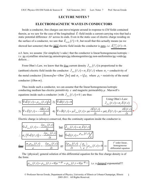
UIUC Physics 436 EM Fields & Sources II Fall Semester, 2011 Lect. Notes 7 Prof. Steven Errede−12Thus, after many charge relaxation time constants, e.g. 20τ relax≤Δ t 1 ps=10 sec, thenρfreert , ≥Δ t = 0 from then onwards}:Maxwell’s equations for a conductor become {with ( ) ∇ , = 01) ∇ i E( r, t)= 02) i B( r t) ∂B rt∇× =−∂t3) E( r,t)( , ) ∂E( r, t)⎛ ∂E r,t∇× B r, t = μσCE r, t + με = μ σCE( r,t)+ ε∂t⎜⎝∂t4) ( ) ( )Now because these equations are different from the previous derivation(s) of monochromaticplane EM waves propagating in free space/vacuum and/or in linear/homogeneous/isotropic nonconductingmaterials {n.b. only equation 4) has changed}, we re-derive the wave equations forE&B∇× to equations 3) and 4): from scratch. As before, we apply ( ) ∂ ∇× ( ∇× E) =− ( ∇× B)∇× ( ∇× B) = μ σC( ∇× E)+ ε ∂ ∇× E∂t∂t 2 ∂ ⎛ ∂E⎞ 22 ∂B∂ B= ∇( ∇iE) −∇ E =− ⎜μσCE+με ⎟ = ∇( ∇iB) −∇ B =−μσC−με2∂t⎝∂t⎠∂t∂t 22 ∂ E ∂E22 ∂ B ∂B= ∇ E = με + μσ2 C= ∇ B = με + μσ2 C∂t∂t∂t∂t2 22 ∂ E( r, t) ∂E( r,t)2 ∂ B( rt , ) ∂Brt( , )Again: ∇ E( r, t)= με + μσ2C and: ∇ B( r, t)= με + μσ2C∂t∂t∂t∂t Note that these 3-D wave equations for E and B in a conductor have an additional term thathas a single time derivative – which is analogous to a velocity-dependent damping term,e.g. for a mechanical harmonic oscillator.( )( ) ( )The general solution(s) to the above wave equations are usually in the form of an oscillatoryfunction * a damping term (i.e. a decaying exponential) – in the direction of the propagation of the EM wave, e.g. complex plane-wave type solutions for E and B associated with the abovewave equation(s) are of the general form:E z t( , )ikz ( −ωt)= E eo ikz ( −ωt)⎛ k ⎞ ˆ 1 B zt , = Beo= ⎜ ⎟k× E zt , = k×E zt ,⎝ω⎠ωand: ( )with {frequency-dependent} complex wave number: k( ω) = k( ω) + iκ( ω)where k( ω) =Re k ( ω)and κ( ω) m k( ω)( ) k k kˆk zˆ(in the ẑ( ω) = ( ω) = ( ω)( )Maxwell’s equations for acharge-equilibrated conductor( ) ( )=I and corresponding complex wave vector k ω = ( k ω + iκ ω )ˆ z.+ direction here), i.e. ( ) ( ) ( )⎞⎟⎠© Professor Steven Errede, Department of Physics, University of Illinois at Urbana-Champaign, Illinois2005-2011. All Rights Reserved.3

UIUC Physics 436 EM Fields & Sources II Fall Semester, 2011 Lect. Notes 7 Prof. Steven ErredeThis can be rewritten as:k⎡1( )μ 2σ 2 2 ⎤Cω⎡ 2 21 ( σ )⎤⎢ ⎥ 2 1⎡C2 σ ⎤C= μεω 1∓1+4( μεω ) ⎢1 1 ⎥ ⎛ ⎞( ) 1 12 ⎢ μεω24 μ 2 42⎥ = ∓ + = ⎢ ∓ + ⎥2 2( εω )2 ⎢ ( εω)⎥ ⎜ ⎟2 ⎢ ⎝εω⎢ ⎥⎠ ⎥⎣⎦ ⎣⎦ ⎣ ⎦2 2( )2Now we can see that on physical grounds ( k > 0 ), we must select the + sign, hence:k21⎡⎛σC ⎞⎤= ( μεω ) ⎢1+ 1+ ⎜ ⎟ ⎥2 ⎢ ⎝εω⎠ ⎥⎣⎦2 2and thus:k12 122 22 εμ⎡⎛σC⎞⎤εμ⎡⎛σC⎞⎤= k = ω ⎢1+ 1+ ⎥ = ω ⎢ 1+ + 1⎥⎜ ⎟ ⎜ ⎟2 ⎢ ⎝εω⎠ ⎥ 2 ⎢ ⎝εω⎠ ⎥⎣ ⎦ ⎣ ⎦2Having thus solved for k (or equivalently, k ), then we can use either of our original two2 2 2relations to solve for κ , e.g. k − κ = μεω , then:2 22 2 2 1⎡2 ⎛σC⎞⎤2 1⎡2 ⎛σC⎞⎤κ = k − μεω = ( μεω ) ⎢1+ 1+ ⎜ ⎟ ⎥− μεω = ( μεω ) ⎢ 1+ ⎜ ⎟ −1⎥2 ⎢ ⎝εω⎠ ⎥ 2 ⎢ ⎝εω⎠ ⎥⎣ ⎦ ⎣ ⎦Thus, we obtain:k( )εμ⎡2 ⎢⎣⎛σ⎞⎜ ⎟⎝εω⎠C( ω) =R e k ( ω)= ω ⎢ 1+ + 1⎥and: ( ) m k( )Note that the imaginary part of k , κ =Im( k)the monochromatic plane EM wave with increasing z:E z t = E e e( , )o−κ z ikz ( −ωt)2and: ( )⎤⎥⎦1 22εμ⎡⎛σC ⎞⎤κ ω =I ( ω ) = ω ⎢ 1+ ⎜ ⎟ −1⎥2 ⎢ ⎝εω⎠ ⎥⎣⎦ results in an exponential attenuation/damping of ( ) 1 −κz−ω 1 −κzB z, t = Boe e = k× E( z,t)= k×Eoe eωω( −ω)ikz t ikz tn.b. these solutions satisfy the above wave equations for any choice ofThe characteristic distance over whichE o . E and B are attenuated/reduced to11 e= e − = 0.3679δ ω ≡ 1 κ ω (SI units: meters).of their initial values (at z = 0) is known as the skin depth, ( ) ( )sc1 2i.e. δ ( ω)sc1 1= =κ( ω)2εμ⎡ σ ⎤Cω ⎢⎛ ⎞1+ ⎜ ⎟ −1⎥2 ⎢ ⎝εω⎠ ⎥⎣⎦1 2⇒( δ , )−1ikzE z =sct = Eoe e( δ , )−1ikzB z =sct = Boe e( −ωt)( −ωt)© Professor Steven Errede, Department of Physics, University of Illinois at Urbana-Champaign, Illinois2005-2011. All Rights Reserved.5

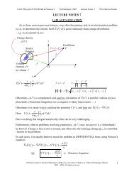
UIUC Physics 436 EM Fields & Sources II Fall Semester, 2011 Lect. Notes 7 Prof. Steven Errede( )The real part of k , i.e. k( ω) =Re k ( ω)determines the spatial wavelength λ ( ω ),the propagation speed v( ω ) of the monochromatic EM plane wave in the conductor, and also theindex of refraction:2π2πλ( ω)= =k R v( ω)and: n( ω)( )( ω) e k( ω)ω ω= =k R ( )( ω) e k( ω)( )()( ω) cRe k( ω)c ck= = =v ω ω ωThe above plane wave solutions satisfy the above wave equations(s) for any choice of E o .As we have also seen before, it can similarly be shown here that Maxwell’s equations 1) and 2) ( ∇ iE= 0 and ∇ i B=0)rule out the presence of any {longitudinal} z-components for E and B (for EM waves propagating in the + ẑ -direction) ⇒ E and B are purely transverse waves(as before), even in a conductor!If we consider e.g. a linearly polarized monochromatic plane EM wave propagating in thez ikz ( tẑE −κ −ωz,t = E e e )ˆ x , then:+ -direction in a conducting medium, e.g. ( ) 1 ⎛ k⎞−κzikz ( −ωt) ⎛k+iκ⎞ −κzikz ( −ωt)B ( zt , ) = k× E( zt , ) = ⎜ ⎟Ee ˆˆoe y=⎜ ⎟Ee oe yω ⎝ω⎠⎝ ω ⎠⇒ E( z, t) ⊥ B( z,t) ⊥ zˆ( + ẑ = propagation direction)oThe complex wavenumber = + = where:ik k ik Ke φ 2 2and ( )−1φk≡ tan κK ≡ k = k + κkIn the complex k -plane:()κ = Im kκ Kφk k = Re( k)k2 2K = k= k + κ6© Professor Steven Errede, Department of Physics, University of Illinois at Urbana-Champaign, Illinois2005-2011. All Rights Reserved.

UIUC Physics 436 EM Fields & Sources II Fall Semester, 2011 Lect. Notes 7 Prof. Steven ErredeThen we see that: ( , )and that: ( , )z ikz ( tE −κ −ωzt = Ee e )ˆ x has: iE = E e δEo −κzi( kz−ωt) k −κzi( kz−ωt)has:B zt = Be ˆ ˆ0e y= Eeoe yω io ok = Ke φki ki kφKeBB δo= Beo= Eo= Eeoω ωiφk2 2iδ Ke iδ K i( δ + φ ) k + κ i( δ + φ )Thus, we see that: Be = Ee = Ee = Eeω ω ω i.e., inside a conductor, E and B are no longer in phase with each other!!!Phases of E and B : δ = δ + φB E kBBE k E ko o o oWith phase difference: ΔϕB−E ≡δB− δE= φk⇐ magnetic field lags behind electric field!!!2BoK⎡⎛σC ⎞⎤1We also see that: = = ⎢εμ1+ ⎜ ⎟ ⎥ ≠Eoω ⎢ ⎝εω⎠ ⎥ c⎣⎦ The real/physical E and B fields associated with linearly polarized monochromatic planeEM waves propagating in a conducting medium are exponentially damped:( ) ( ) ˆ −κz( , ) =R ( , ) =ocos − ω + δEδ = δ + φB E kE zt e E zt Ee kz t x( ) ( )1 2B zt , =R e B zt , = Be cos kz− t+ y= Be cos kz− t+ + yˆ−κz−κz( ) ( ) ˆoω δB oω { δE φk}( )δi EBEooK ( ω)⎡⎛σC ⎞= = ⎢εμ1+ ⎜ ⎟ω ⎢ ⎝εω⎣⎠2⎤⎥⎥⎦12⎡⎛σC ⎞ω ≡ ω = ω + κ ω = ω⎢εμ1+ ⎜ ⎟⎢ ⎝εω⎣⎠2 2where K( ) k( ) k ( ) ( )2⎤⎥⎥⎦1 2δBδE φk= + , φ ( ω)k( )( ω)⎛ −1κ ω ⎞≡ tan⎜k ⎟⎝ ⎠Definition of the skin depth δ ( )sc and k( ω) = k( ω) + iκ( ω)z , k( ) ω = k( ω) = k( ω) + iκ( ω)ω in a conductor:( )ˆδsc( ω)1 1≡ =κ( ω)2εμ⎡ σ ⎤Cω ⎢⎛ ⎞1+ ⎜ ⎟ −1⎥2 ⎢ ⎝εω⎠ ⎥⎣⎦1 2=Distance over which the E and B fields fall to11 e= e − = 0.3679 oftheir initial values.The instantaneous power per unit volume in the conductor {ultimately dissipated as heat!} is: − κp z, t = J z, t iE z, t = σ E z, t iE z, t = σ E z, t = E e z cos kz− ωt+δ Watts m2 2 2 2 3( ) ( ) ( ) C ( ) ( ) C ( ) o ( E) ( )p zt ,1 2 2The time-averaged power per unit volume in the conductor is thus: ( ) −t=2zEe κo© Professor Steven Errede, Department of Physics, University of Illinois at Urbana-Champaign, Illinois2005-2011. All Rights Reserved.7

UIUC Physics 436 EM Fields & Sources II Fall Semester, 2011 Lect. Notes 7 Prof. Steven ErredeSpecial/Limiting Cases:a) Good conductors: σCSince k = k+ik and σC εω Conductivity of good conductor σ → ∞ ( ie .. ρ = 1σ→ 0).σ C⎛ ⎞ εω , i.e. ⎜ 1⎟⎝εω ⎠then:1 12 212 2 2C C CC C Cεμ⎡⎛σ ⎞⎤εμ⎡⎛σ ⎞⎤εμ ⎡ σ ⎤ ε μσk ≡ ω ⎢ 1+ ⎜ ⎟ + 1⎥ ω ⎢ 1+ ⎜ ⎟ ⎥ ω ⎢ ⎥ = ωCωμσ C2 ⎢ ⎝εω ⎠ ⎥ 2 ⎢ ⎝εω ⎠ ⎥ 2 ⎣ εω⎣ ⎦ ⎣ ⎦⎦ 2 ε ω = 2and:1 12 212 2 2C C Cεμ⎡⎛σ ⎞⎤εμ⎡⎛σ ⎞⎤εμ ⎡ σ ⎤ ε μσκ ≡ ω ⎢ 1+ ⎜ ⎟ − 1⎥ ω ⎢ 1+ ⎜ ⎟ ⎥ ω ⎢ ⎥ = ωCωμσ C2 ⎢ ⎝εω ⎠ ⎥ 2 ⎢ ⎝εω ⎠ ⎥ 2 ⎣ εω⎣ ⎦ ⎣ ⎦⎦ 2 ε ω = 2∴ In a good conductorσC εω :kωμσ2C( ω) κ( ω) and skin depth: δ ( ω)sc≡ 1 2κ ω ωμσ.( )C8© Professor Steven Errede, Department of Physics, University of Illinois at Urbana-Champaign, Illinois2005-2011. All Rights Reserved.

UIUC Physics 436 EM Fields & Sources II Fall Semester, 2011 Lect. Notes 7 Prof. Steven ErredeFORMULAS FOR EM WAVE PROPAGATION IN A GOOD CONDUCTORkωμσ2C( ω) κ( ω) and: δ ( ω)2πWavenumber, k ( ω)≡ ⇒ ( )λ ( ω)n.b. in a perfect conductor:⇒ ( ) ( )CCsc1 2= skin depth ≡ κ ω ωμσ( ) ( )( )2π2π2λ ω = = 2πδsc( ω)= 2πk ω κ ω ωμσσ = ∞ φ ( ω) ( δ δ )k B E( )( ω)⎛κ ω ⎞≡ − ≡ ⎜k ⎟⎝ ⎠ωμσ−1 πk ω κ ω = =∞ But: tan () 1 = 45 =242π πλ ω = = 0⇒ φ = δB− δE= 45 =k ω4⇒ ( )δsc( ω)( )( )= 1 2 0κ ω ωμσ=⇒ B lagsCCC()−1 −1tan tan 1E by 45 in a good conductor. πn.b. In a perfect conductor: σC=∞, φ ≡ 45 =4In a typical good conductor (e.g. gold/silver/copper/…): ( σ εω) 116For optical frequencies/visible light region: ω 10 radians sec . A good conductor typically has7σC 10 Siemens m and ε 3εo , and at optical frequencies: ( ) 37.7 1Cσ εω is satisfied.If the conductor is non-magnetic (e.g. copper, aluminum, gold, silver, platinum… etc.)−7⇒ μ μ = 4π×10 Henrys/m .Then: k ( ω) κ( ω)o116 −7 7 2ωμσCωμoσ ⎡C10 × 4π× 10 × 10 ⎤8 ≈ = 2.51×10 radians/m2 2⎢2⎥ ⎣⎦−8λ ω = 2π k ω = wavelength in good conductor 2.51× 10 m=25.1 nmAnd: ( ) ( )82π 2πcc 2π× 3×10−7cf w/ vacuum wavelength: λo= = = = 1.885× 10 m=188.5 nm16k ω f 10goodvacuum⇒ λ( ω) 25.1 nm( conductor ) λo= 188.5 nm( wavelength )o⎛ λ ⎞o188.5 nmVacuum/conductor λ-ratio:⎜= 7.52λ( ω)⎟ at optical frequencies,⎝ ⎠ 25.1 nm1 λ( ω) −9Skin depth: δsc ( ω)= 4.0× 10 m=4.0 nm !!!κ( ω)2π⇒ This explains why metals are opaque at optical frequencies,{and also explains why/how silvered sunglasses work!}C16ω ≈ 10 radians/sec16ω ≈ 10 rad/sec.© Professor Steven Errede, Department of Physics, University of Illinois at Urbana-Champaign, Illinois2005-2011. All Rights Reserved.9

UIUC Physics 436 EM Fields & Sources II Fall Semester, 2011 Lect. Notes 7 Prof. Steven ErredeCompare these results for EM waves propagating in conductors at optical frequencies to thosefor EM waves propagating in conductors, but with very low frequencies – e.g. the AC linefrequency, f = 60 Hz ⇒ ω = 2π f = 120 π rad/sec , where the criterion for a goodACconductor, ( )15ACσ εω 10 1 is certainly well-satisfied:CACf−7 7⎧ ωμσ ⎡C120π× 4π× 10 × 10 ⎤kACκAC⎪ = 48.7 /2⎢2⎥ = radians m⎪⎣⎦⎪ 2π⎪λAC= = 0.129 m=12.9 cmk⎪λ = × m⎪6⎪λo5×10 mAC7= 3.87×10 !!⎪ λAC0.129 m⎪⎪AC λAC−260 Hz AC skin depth: δsc= 2.05× 10 m=2.05 cm!!⎪⎩2π6At = 60Hz: ⎨ o5 10 !!AC⇒ Need at least 3-4× ≈ several → 10 cm to screen out unwanted 60 Hz AC signals !!δsc⎛ ⎞Instantaneous EM Wave Energy Densities in a Good Conductor: ⎜ ⎟ 1⎝εω⎠ EM EM ⎛1 2⎞ ⎛ 1 2⎞ ⎛1 ⎞⎛ 1 π⎞ φk ≡ δB − δE =uEM = uE + uM= ⎜ εE ⎟+ ⎜ B ⎟= ⎜ εEiE⎟+⎜ BiB⎟⎝2 ⎠ ⎝2μ⎠ ⎝2 ⎠ ⎝2μ⎠ {in a good conductor}−κE z, t E e z−κ= cos kz− ωt+δ x B zt , = Be z cos kz− ωt+ δ + φ y( ) ( ) ˆWhere:o12 2K ( )⎡⎤⎢⎛ C ⎞o oεμ 1 ⎥oEω σ ε μσCB = E = + ⎜ ⎟ E ω ⎢ ⎝εω⎠ ⎥ ε ω⎣⎦And: k ( ω) ( )Then:v( ω)ωμσC κ ω ≈ ,2σ Cand ( ) ( ) ˆω ω 2ωc= = = for a good conductor.k( ω) ωμσ ωσCCn( ω)2oE( ) 445μσC= E o for a good conductor,ω1 1 EM1( ) 2 2 −, 2 κ zu cos2Ez t = ε E = εEi E = εEoe ( kz− ωt+δE)and:2 2 21 1 EM 12 2 −, 2 κz σcos 2 C 2 − 2 κzu cos2Mz t = B = BiB= Boe kz− ωt+ δE + φk Eoe kz− ωt+ δE + φk2μ 2μ 2μ 2ω( ) ( ) ( )10© Professor Steven Errede, Department of Physics, University of Illinois at Urbana-Champaign, Illinois2005-2011. All Rights Reserved.

UIUC Physics 436 EM Fields & Sources II Fall Semester, 2011 Lect. Notes 7 Prof. Steven Errede1≡τ ∫τu z t dtTime-averaging these quantities over one complete cycle: u( z, t) ( , )1 2 2 1 τ− κ z21 2 −2zu ( z, t) = ε E e cos ( kz− ωt+ δ ) dτ= ε Eeo∫κ4EME2oτ0E1=2σ 2 2 1 τC − κ z21 ⎛σC ⎞ 2 −2zu ( z, t) = E e cos ( kz− ωt+ δ + φ ) dτ= ⎜ ⎟Ee o∫κ4 ⎝ ω ⎠EMM2ωoτ0E k1=2EM EM EM 1 ⎛ σ ⎞ zuTot z, t = uE z, t + uM z, t = ε ⎜1+⎟Eoe κ4 ⎝ εω ⎠C 2 −2∴ ( ) ( ) ( )σ C⎛ ⎞But: ⎜ ⎟ 1εω1⎛σ⎞⎡1zu z,t ε E e κ ⎤ ⎜⎝⎟⎢⎠⎣⎥⎦⎝ ⎠ for a good conductor, ⇒ EM( ) C2 −2Toto2 εω 2( z,t)( z,t)0n.b. Exponentially attenuated in z !!!EMuM⎛σC ⎞i.e. the ratio:= 1EM ⎜uεω ⎟E ⎝ ⎠ or EM( , ) EMu ( , )Mz t uEz t for a good conductor.⇒ Vast majority of EM wave energy is carried by the magnetic field in a good conductor !!!Poynting’s Vector: 1 S = E×Bμ 1 1κ zS z, t = E× B = E cos ˆoBoe φkzμ 2μ−2⇒ ( )πφk=4 1 1 κzKI z = S z, t = EoBoe − cosφk = Eoe− ⎛ ⎜ cosφ⎞k ⎟2μ 2μ ⎝ω⎠2κz2 2EM wave intensity (aka irradiance): ( ) ( )But:ωμσ C2KcosφkμσC= =ω ω ω 2ω 1 ⎛ k ⎞ 1 σI z = S z,t = ⎜ ⎟Eoe = Eoe2μ ⎝ω⎠2 2μω2 −2κzC 2 −2 ∴ ( ) ( )κzb.) Special/Limiting Case of a Fair Conductor:c.) Special/Limiting Case of a Poor Conductor: (i.e. an insulator):Here:σCσ C⎛ ⎞ εω , i.e. ⎜ ⎟ 1⎝εω⎠Complex wavenumber: k = k+iκσC≈ εω ⇒ Must use exact formulae! . Conductivity of poor conductor: σ 0 ( ie . . ρ 1 σ ) , with k = Re ( k ) and Im( k )κ = .→ = →∞ .C C Ck( )121 12 2 2 2 2C1C1Cεμ⎡⎛σ ⎞⎤εμ ⎡ ⎛σ ⎞ ⎤ εμ ⎡ ⎛σ⎞ ⎤ω ≡ ω ⎢ 1+ ⎜ ⎟ + 1⎥ω ⎢1+ ⎜ ⎟ + 1⎥ = ω ⎢2+⎜ ⎟ ⎥ ω εμ2 ⎢ ⎝εω ⎠ ⎥ 2 ⎢⎣ 2⎝εω ⎠ ⎥⎦ 2 ⎢⎣ 2⎝εω⎣⎦⎠ ⎥⎦∴ ( ) k ω ω εμ for a poor conductor.© Professor Steven Errede, Department of Physics, University of Illinois at Urbana-Champaign, Illinois2005-2011. All Rights Reserved.11

UIUC Physics 436 EM Fields & Sources II Fall Semester, 2011 Lect. Notes 7 Prof. Steven ErredeLikewise:1 21 2ε2εμ⎡ σ ⎤2⎛( ) 1 C ⎞εμ ⎡ 1κ ω ω ⎢1⎥⎛σ ≡ + ⎜ ⎟ − ω 1C ⎞ ⎤2μσ+ ⎜ ⎟ −1= ωC1 μ⎢⎥σ2 22 ⎢ ⎝εω⎠ ⎥ 2 2 εω⎣⎦ ⎢⎣⎝ ⎠ ⎥⎦4εω 2 C ε1 μ∴ κ( ω) σ for a poor conductor.2 C ε1μ⎛σ In a poor conductor C ⎞⎜ ⎟ 1⎝εω⎠ , the ratio: ⎛ 2σκ( ωC) ⎞ ε 1 ⎛σC ⎞⎜1k ( ω)⎟ = ⎜ ⎟ i.e. κ( ω) k ( ω).⎝ ⎠ ω εμ 2 ⎝εω⎠⇒ Complex wavenumber k ≡ k+iκ is primarily real, because κ k in a poor conductor.⎛1κ ω ⎞−−1⎛1⎛ωC⎞⎞1⎛σC⎞Phase angle in a poor conductor: φk ≡δB − δE= tan⎜tan 1k ( ω)⎟= ⎜ ⎜ ⎟⎟⎜ ⎟⎝ ⎠ ⎝2⎝εω⎠⎠2⎝εω⎠ ⇒ δ B= δ E+ φ k δ E, i.e. B and E are nearly in phase with each other in a poor conductor(i.e. losses very small in a poor conductor).In a typical poor conductor, e.g. pure water:Water has a huge static electric permittivity (due to permanent electric dipole moment ofεHO 81ε at zero Hz, . . 02oie f = ( at P= 1 ATM and T = 20 C), however, at16−1210 rad sec ε ω ≈ 1.777ε, where ε o= 8.85× 10 Farads m .water molecule): ( )ω ≈ : ( )optical frequencies ( )H2O( )−7Since water is non-magnetic: μHOμo= 4π× 10 Henrys m⇒ index of refraction: ( ) ( )2n ω = ε ω μ ε μ 1.333 at optical frequencies.HO 2 HO 2 HO 2 o oHO 2 HO 2 5 −6The conductivity of pure water is: σC = 1 ρC 1 2.5× 10 Ω -m= 4.0×10 Siemens m−11( at P= 1 ATM and T = 20 C). Thus, the criteria for a poor conductor ( σCεω) 2.54×10 1is certainly satisfied at optical frequencies.The wavenumber in pure HO2at optical frequencies is:kHO 2( )ω ω εμ ≈ ω εμ = 10 1.777× 8.85× 4π× 10 4.45×10o16 −7 7oradians m−7The wavelength in pure HOis: λ 2 1.413 10 141.32 HO= π k2 HO= × m= nm at optical frequencies.2−7cf w/ the vacuum wavelength: λo = c f = 2πc ω = 1.885× 10 m=188.5 nm12© Professor Steven Errede, Department of Physics, University of Illinois at Urbana-Champaign, Illinois2005-2011. All Rights Reserved.

UIUC Physics 436 EM Fields & Sources II Fall Semester, 2011 Lect. Notes 7 Prof. Steven Errede⎛ λ ⎞o188.5 nmNote that the optical wavelength ratio: = = 1.333 = n⎜2λ ⎟⎝ HO141.3 nm2 ⎠since λ = λ n in a poor conductor!!!H2O o H2OH O,Skin depth: δ ( ω)sc≡ 1 1κ ω σ μεfor a poor conductor ⎛ ⎞⎜ ⎟⎝εω⎠ 1 .( )1For pure H 2 O at optical frequencies:1 μ 1 μ 1 1 4π×10κ ω σ σ2 ε 2 ε 2 ⎝2.5× 10 ⎠ 1.777× 8.85×102C−7o ⎛ ⎞−4HO( ) 5.65 102C≈C= ⎜× rad m5 ⎟−12σ CδHO 2sc( ω)1≡ = × m=κHO 231.7688 10 1.77kmn.b. neglects/ignores Rayleigh scattering process – visible lightvisphotons elastically scattering off of H 2 O molecules. λ 10attenmRatio:1 μ⎛κ ( )CHOω ⎞ σ1 1 1 12 2 ε ⎛σC ⎞ ⎛ ⎞= = = = ×⎜ 5 −12 16k HO ( ω)⎟ ω εμ 2⎜εω⎟ ⎜ ⎟⎝⎝ ⎠ 2 ⎝2.5× 10 ⎠1.777× 8.85× 10 × 102 ⎠−111.27 10 1−1 HO 2−11Phase difference: φ ≡δ − δ = tan ⎜ ⎟ 1.27×10 radians ( 1)k B E⎛κ⎜⎝k HO 2⎞ i.e. δB= δE + φk δE⎟⎠ ⇒ B and E are nearly in phase with each other in pure H2 O at optical frequencies.For pure H 2 O at low frequencies – e.g. 60 Hz AC line frequency ( ω 2π f 120πrad sec)ACThe electric permittivity at f = 60 Hz is ε ( )HO 2AC= = :−12f 60Hz 80εo= 80× 8.85×10 Farads mAC−7HO 2 −6and μ μ = 4π×10 Henrys m. Conductivity of pure HO:2σ C= 4.0×10 Siemens mHO 2oACNote that the criteria for a poor conductor:⎛6σ ⎞−C4.0×1015 1AC ⎜ −12εHOω ⎟⎝80 8.85 10 1202 AC⎠× × ⋅ πis not satisfied at the 60 Hz AC line frequency – i.e. at low enough frequencies,even poor conductors such as pure water are actually quite good conductors !!!Thus, for the following, we must use the good conductor approximations:−7 −6ω μ σ ω μ σ 120π ⋅ 4π× 10 ⋅ 4×10≈ = = ×2 2 2HO 2HO 2 HO 2AC AC C AC o Ck AC ( ω) κ AC ( ω)λHO 2AC( ω)HO 2k AC( )−53.08 10 rads m 2π52.04 10 mω = × cf w/ vacuum wavelength: 2πc6λo= c fAC= = 5.00×10 mωAC© Professor Steven Errede, Department of Physics, University of Illinois at Urbana-Champaign, Illinois2005-2011. All Rights Reserved.13

UIUC Physics 436 EM Fields & Sources II Fall Semester, 2011 Lect. Notes 7 Prof. Steven ErredeVacuum/good conductor wavelength ratio:⎛ λ ⎞o5.00×10⎜ HO⎟=2⎝λAC⎠ 2.04×1065m 24.495mAC AC4Skin depth for pure H 2 O at 60 Hz AC line frequency: δHO≡ 1 κ 3.25 10 32.52 HO× m=km2This may seem like a large distance scale associated with the attenuation of the 60 Hz EMwaves propagating in pure water, however compare the skin depth to the wavelength at thisACHO 2 6AC ACfrequency: δ = 32.5 km vs. λ = 1.77× 10 m , i.e. we see that δ λ , as we expectHO 2for the case of a good conductor !!!AC ACThe ratio ( κHOkHO)2 2ACH2OH2O 1 for pure H 2 O at 60 Hz AC line frequency, which is what we expect fora good conductor {this ratio should be 1 for a poor conductor}.π≡ − = tan tan 1 = = 454which again is what we expect for a good conductor, i.e. B lags E by 45 o !− AC AC−Thus, the phase difference is: φ δ δ ( κ k ) ()1 1 ok B E H2O H2O⎛ ⎞Instantaneous EM energy densities in a poor conductor: ⎜ ⎟ 1⎝εω⎠ ⎛1 ⎞ ⎛ 1 ⎞ ⎛1 ⎞⎛ 1 ⎞= + = ⎜ ⎟+ ⎜ ⎟= ⎜ ⎟+⎜ ⎟⎝2 ⎠ ⎝2μ⎠ ⎝2 ⎠ ⎝2μ⎠EMEM( , ) ( , ) ( , )2 2uEM z t uE z t uMz t εE B εEiE BiBσ CThe physical E and B fields are:−κE z, t = E e z cos kz− ωt+δ x( ) ( ) ˆoE−κand B( zt , ) = Be z cos( kz− ωt+ δ + φ ) yˆo E k1 22K⎡ σ ⎤Cwhere: Bo E ⎢⎛ ⎞oεμ 1 ⎥⎛σ = = + ⎜ ⎟ Eo ≈ εμ Eofor a poor conductor, C ⎞⎜ ⎟ 1ω ⎢ ⎝εω⎠ ⎥εω⎣⎦⎝ ⎠ .ω1k ω εμ = where: v cv= εμ= nand: εμn = for a poor conductor.εoμo1 μand: κ σ k ω εμ , K ≡ k ω εμ for a poor conductor.2 c ε1 1 1Eio E and:2 2 21 1 EM1( ) 2 2 −, 2 κ zu cos2Mz t = B = BiB= Boe ( kz− ωt+ δE + φk)2μ 2μ 2μEMThen: ( ) 2 2 − 2 κ zu z, t = ε E = cE E = εE e cos2( kz− ωt+δ )Time-averaging these quantities:EM 1uEz t Eoe κ41 z 1uMz t = Boe κ εμ4μ4 μ2 −2zEM2 −2( , ) = ε and: ( , )2 −2κz1 2 −2( ) Eeo= ε Eeo4κz14© Professor Steven Errede, Department of Physics, University of Illinois at Urbana-Champaign, Illinois2005-2011. All Rights Reserved.

UIUC Physics 436 EM Fields & Sources II Fall Semester, 2011 Lect. Notes 7 Prof. Steven Errede1 1 1uTot z, t = uE z, t + uM z,t εEo e + εEo e = εEoe4 4 22 −2 2 −2 2 −2∴ ( ) ( ) ( )EM EM E κ z κz κz1zuTotz,t Eoe κ⎛ ⎞= ε for a poor conductor ⎜ ⎟ 12⎝εω⎠ .EM2 −2Thus: ( )The ratio of {time-averaged} electric/magnetic energy densities for a poor conductor:1 2 −2κzEMu ( , )oEz t ε Ee4 κ = 1 φEMkδB δ⎛ ⎞− 1 μ≡ −E= ⎜ ⎟u ( , ) 1 2 2 zMz t− κε Ee⎝ ⎠o4 ⇒ EM wave energy is shared ≈ equally by the E and B fields in a poor conductor!σ C1 HO 2otan 1 κH⎜ k HO⎟2O σc kH2O ω εμo2 ε2Instantaneous Poynting’s Vector for EM waves propagating in a poor conductor: 1 S z t E z t B z tμ( , ) = ( , ) × ( , ) 1 ε κ zS z,t E ˆoe z for a poor conductor.2 μ2 −2∴ ( )oIntensity of EM waves propagating in a poor conductor: 1 ε 2 −2zI ( z) = S( z,t) = Eoe κ2 μo 1 εμS z, t = E z, t × B z, t E e cosφzˆμ2μo 2 −2κz⇒ ( ) ( ) ( ) oko≈1© Professor Steven Errede, Department of Physics, University of Illinois at Urbana-Champaign, Illinois2005-2011. All Rights Reserved.15

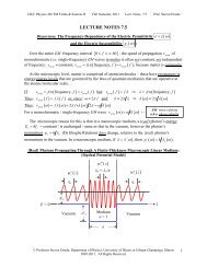
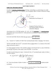
UIUC Physics 436 EM Fields & Sources II Fall Semester, 2011 Lect. Notes 7 Prof. Steven ErredeReflection of EM Waves at Normal Incidence from a Conducting Surface:In the presence of free surface charges σfreeand/or free surface currents, K freethe boundaryconditions obtained from (the integral forms of) Maxwell’s equations for reflection andrefraction at e.g. a dielectric-conductor interface become:BC 1): (normal D ⊥ ⊥at interface): ε1E1 − ε2E2 = σfreeBC 2): (tangential E at interface): E1 − E2 = 0E= E ⇒ 1 2⊥ = normal to plane of interface = parallel to plane of interfaceBC 3): (normal B ⊥ ⊥⊥at interface): B1 − B2 = 0 ⇒ B1 = B2⊥BC 4): (tangential H at interface):1 1 B − B = K ˆfree× nμ|| ||1 21μ2→21where ˆn → is a unit vector ⊥ to the interface, pointing from medium (2) into medium (1).21{n.b. do not confuse ˆn → with the EM wave polarization vector ˆn !!!}21 Note: For Ohmic conductors (i.e. “normal” conductors obeying Ohm’s Law Jfree= σCE)there can be no free surface currents, i.e. Kfree= 0 because Kfree≠ 0 would require an infiniteE -field at the boundary/interface!Suppose ∃ a boundary/interface (located in the x-y plane at z = 0) between a non-conductinglinear/homogeneous/isotropic medium (1) and a conductor (2). A monochromatic plane EMwave is incident on the interface, that is linearly polarized in + ˆx direction, traveling in the+ ẑ direction, approaching the interface/boundary from the left, in medium (1) as shown in thefigure below:16© Professor Steven Errede, Department of Physics, University of Illinois at Urbana-Champaign, Illinois2005-2011. All Rights Reserved.

UIUC Physics 436 EM Fields & Sources II Fall Semester, 2011 Lect. Notes 7 Prof. Steven Erredeikz ( 1 t)Incident EM wave {medium (1)}: E −ω( z,t)= E e xˆand: ( , )inci( k1z t)Reflected EM wave {medium (1)}: E − =ω( z,t)= E e xˆand: ( , )refloincoreflikz 1Binczt = Eoe yincv1 1 ikz (2 −ωt)Transmitted EM wave {medium (2)}: E ( z,t)= E e xˆand: ( , )transotransn.b. complex wavenumber in {conducting} medium (2): k2= k2 + iκ2 In medium (1) EM fields are: E ( z, t) = E ( z, t) + E ( z,t)Tot1inc reflIn medium (2) EM fields are: E ( z, t) = E ( z,t)Tot2transApply BC’s at the z = 0 interface in the x-y plane:( − −ω )i k1z tBreflzt =− Eoe yreflv1 k2ikz (2 −ωt)B ˆtranszt = Eoe ytransω and: B ( zt , ) = B ( zt , ) + B ( zt , )and: B ( zt , ) = B ( zt , )Tot2Tot1inc refl⊥ ⊥BC 1): ε1E1 − ε2E2 = σfree but: E⊥ 1= E 1= 0 and: E⊥ = E = 0 ∴ 0 − 0 = σ ⇒ σ 02 2 freefree=zztrans( )1B = k ˆ × Ev 1 ( −ωt)ˆˆ BC 2): E1 = E2E + E = E∴ o inc o refl o trans⊥ ⊥BC 3): B1 = B2but: B⊥ = 1B = 10 and: B⊥ = B = 0 ⇒ 0=02 2zBC 4):1 || 1 ||1k2B ˆ1− B2= Kfree× n→but: Kfree= 0 ∴ ( E o− E )inc o− Erefl otransμ211μ2μ1v1 μ2ω= 0or: E o− E inc o= β E ⎛μ1vk⎞ ⎛1 2μ1v⎞1refl oβ ≡ ⎜ ⎟=ktrans⎜ ⎟ 2⎝ μω2 ⎠ ⎝μω2 ⎠⎛1−Thus we obtain: Eβ ⎞o= Erefl⎜ ⎟2oinc⎝1+and: Eo= Etransoincβ ⎠( 1+ β )or:⎛E⎞o ⎛refl 1− β ⎞ ⎛E⎞o 2⎛μ⎟=⎜⎜ ⎟E⎟⎝o1+and:trans=1vkβinc ⎠ ⎝ ⎠⎜ Ewith: ⎞ ⎛1 2μ1v⎞1β ≡ k⎟⎝ o ( 1+⎜ ⎟=⎜ ⎟βinc ⎠ )⎝ μω2 ⎠ ⎝μω2 ⎠Note that these relations for reflection/transmission of EM waves at normal incidence on anon-conductor/conductor boundary/interface are identical to those obtained for reflection /transmission of EM waves at normal incidence on a boundary/interface between two nonconductors,except for the replacement of β with a now complex β for the present situation.z2© Professor Steven Errede, Department of Physics, University of Illinois at Urbana-Champaign, Illinois2005-2011. All Rights Reserved.17

UIUC Physics 436 EM Fields & Sources II Fall Semester, 2011 Lect. Notes 7 Prof. Steven ErredeFor the case of a perfect conductor, the conductivity σ = ∞ {thus resistivity, ρ = 1σ= 0}⇒ bothand since:ωμ2σCk2 κ 2 =∞ and since: k2 = k2 + iκ22⎛μ1vk⎞ ⎛1 2μ1v⎞1β ≡ ⎜ ⎟=k⎜ ⎟ 2 ⇒ β = ∞⎝ μω2 ⎠ ⎝μω2 ⎠C then: k = ∞+ i∞=∞ ( + i )C21Thus, for a perfect conductor, we see that: E o=−E andrefl oE = 0 and thus for a perfectinctransconductor the reflection and transmission coefficients are:C22 *⎛Eo ⎞ E ⎛refl oE ⎞⎛refl oE⎞refl oreflR ≡ = = ⎟⎜ = 1⎜ E ⎟oE ⎜inc oE ⎟⎜inc oE⎟⎝ ⎠ ⎝ inc ⎠⎝oinc⎠and: T = 1− R = 0We also see that for a perfect conductor, for normal incidence, the reflected wave undergoes a180 o phase shift with respect to the incident wave at the interface/boundary at z = 0 in the x-yplane. A perfect conductor screens out all EM waves from propagating in its interior.For the case of a good conductor, the conductivity σCis finite-large, but not infinite.The reflection coefficient R for monochromatic plane EM waves at normal incidence on a goodconductor is not unity, but close to it. {This is why good conductors make good mirrors!}For a good conductor:⎛Eo ⎞ E ⎛refl oE ⎞⎛refl oE ⎞refl orefl1− β ⎛1− β ⎞⎛1− β ⎞R ≡ = = ⎟⎜ = =⎜ E ⎟oE ⎜⎜ ⎟⎜ ⎟1 1 1inc oE ⎟⎜inc oE ⎟⎝ ⎠ ⎝ inc ⎠⎝o+ β + β + βinc ⎠⎝ ⎠⎝ ⎠2 2 *2 *Where:⎛μvk⎞ ⎛ μv⎞⎝ ⎠ ⎝ ⎠ 1 1 2 1 1≡ ⎜ ⎟=⎜ ⎟k2μω2μωand: k= k + iκ2 2 22β. For a good conductor:kκ2 2ωμ2σC2⎛ μv⎞ ⎛ μv⎞ ωμ σσ⎜ ⎟ 2 ⎜ ⎟1 1⎝μω 2 ⎠ ⎝μω 2 ⎠ 2 2μω2Thus: 1 1 1 1 2 CCβ = k = ( 1+ i) = μ v ( 1+i)Define: γ μ1v1σC2μ ω≡ Then: β = γ ( 1+i)2Thus, the reflection coefficient R for monochromatic plane EM waves at normal incidence ona good conductor is:with: γ ≡ μ1v12 2 * 2 2E o( 1refl 1− β ⎛1− β ⎞⎛1− β ⎞ ⎛1−γ −iγ ⎞⎛1− γ + iγ⎞ ⎡ − γ ) + γ ⎤R = = = =2 2E ⎜ ⎟⎜ ⎟ ⎜ ⎟⎜ ⎟=⎢ ⎥o1+ β 1+ β 1+ β 1+ γ + iγ 1+ γ −iγ( 1+ γinc⎝ ⎠⎝ ⎠ ⎝ ⎠⎝ ⎠ ⎢⎣ ) + γ ⎥⎦σC2μ ω218© Professor Steven Errede, Department of Physics, University of Illinois at Urbana-Champaign, Illinois2005-2011. All Rights Reserved.

UIUC Physics 436 EM Fields & Sources II Fall Semester, 2011 Lect. Notes 7 Prof. Steven ErredeObviously, only a small fraction of the normally-incident monochromatic plane EM wave istransmitted into the good conductor, since R < 1 and T = 1− R , i.e.:T( 1 γ)( 1 γ)2⎡2− + γ ⎤= 1− R= 1 −⎢ 12⎥2⎢⎣+ + γ ⎥⎦( )Note that the transmitted wave is exponentially attenuated in the z-direction; the E andB fields in the good conductor fall to 1/e of their initial {z = 0} values (at/on the interface) afterthe monochromatic plane EM wave propagates a distance of one skin depth in z into theconductor:δsc( ω)1 2≡ κ ω ωμ σ( )2 2Note also that the energy associated with the transmitted monochromatic plane EM wave isultimately dissipated in the conducting medium as heat.In {bulk} metals, since the transmitted wave is {rapidly} absorbed/attenuated in the metal, wecan only study/measure the reflection coefficient R. A full/detailed mathematical description of thephysics of reflection from the surface of a metal conductor as a function of angle of incidence i.e.k ω = ω v ω = ω c n ω withR ( ω, θinc ) requires the use of a complex dispersion relation ( ) ( ) ( ) ( )complex k ( ω) = k( ω) + iκ( ω)and complex propagation speed v ( ω ) = v ( ω ) + iv ( ω ) = c n( ω )with accompanying complex index of refraction n( ω) = n( ω) + iη ( ω), and thus is fairlycomplicated. So-called ellipsometry measurements of the EM radiation reflected from the surfaceof the metal as a function of angle of incidence yields information on the real and imaginary partsof the complex index of refraction of the metal n( ω) = n( ω) + iη( ω), and thus the real andimaginary parts of the complex dielectric constant and/or the complex electric susceptibility of the2n ω = ε ω ε = 1+ χ ω n ω = ε ω ε = 1+ χ ω .metal, since ( ) ( ) ( ) or ( ) ( ) ( )oeIf interested in learning more about this, e.g. please see/read Optics, M.V. Klein, p. 588-592,Wiley, 1970 {P436 reference book on reserve in the Physics library}. Please see/read also the UIUCP402 Optics/Light Lab Ellipsometry Lab Handout C4 and especially the references at the end.Available at: http://online.physics.uiuc.edu/courses/phys402/exp/C4/C4.pdfWe will discuss the dispersive nature of dielectric, non-conducting materials in the next lecture…Coe© Professor Steven Errede, Department of Physics, University of Illinois at Urbana-Champaign, Illinois2005-2011. All Rights Reserved.19

UIUC Physics 436 EM Fields & Sources II Fall Semester, 2011 Lect. Notes 7 Prof. Steven ErredeFull Maxwell Equations in Matter:The electromagnetic state of matter at a given observation point r at a given time t is describedby four macroscopic quantities:1.) The volume density of free charge: ρ free ( rt , ) 2.) The volume density of electric dipoles: P ( rt , ) ⇐ aka electric polarization 3.) The volume density of magnetic dipoles: M ( rt , ) ⇐ aka magnetization J r,t ⇐ aka {free} current density4.) The free electric current/unit area: ( )freeAll four of these quantities are macroscopically averaged - i.e. the microscopic fluctuationsdue to atomic/molecular makeup of matter have been smoothed out. The four above quantities are related to the macroscopic E and B fields by the four Maxwellequations for matter (see Physics 435 Lect. Notes 24, p. 14): 1i , where: ρboundεoεoD = ε E +Ρ & constitutive relation: D = ε E1) Gauss’ Law: ∇ TotE = ρ = ( ρ + freeρbound)Auxiliary relation:o = −∇ i Ρ ⎛ ε ⎞Electric polarization Ρ= ( ε − εo) E = ε0χeE, electric susceptibility χe= ⎜ −1⎟⎝εo ⎠∇ iD = εo∇ iE +∇ i Ρ= ρfree 2) No magnetic charges/monopoles: ∇ i B = 0 1 Auxiliary relation: H = B−Μ⇒ ∇ iH=−∇i M & constitutive relation: B = μHμo3) Faraday’s Law:B H MEμ0μ ∇× =− =− −0∂t ∂t ∂tMagnetization: ⎛ μ ⎞ ⎛ μ ⎞M − ⎜ ⎟H= χmH, magnetic susceptibility χm= ⎜ − 1 ⎟⎝μo−1⎠⎝μo⎠4) Ampere’s Law: ∇× B = μoJ ToT+ μoJED with JD= ε ∂o∂t mag P magP ∂PTotal current density: JToT = Jfree+ Jbound + JboundJbound= ∇× M J bound= ∂ t ∂P∂E∇× B= μoJfree+ μo∇× M + μo + μoεo∂t∂tDH μoJfreeμ ∂ ∇× = +o∂t20© Professor Steven Errede, Department of Physics, University of Illinois at Urbana-Champaign, Illinois2005-2011. All Rights Reserved.

UIUC Physics 436 EM Fields & Sources II Fall Semester, 2011 Lect. Notes 7 Prof. Steven ErredeWe also have Ohm’s Law: ∂ρJ = σCEand the 3 continuity eqn(s): Jα∇ iα=− ∂ tassociated withα = free, bound and total electric charge conservation.For many/most (but not all!!!) physics problems, e.g. in optics/condensed matter physics,materials of interest are frequently non-magnetic (or negligibly magnetic) and have no (free) charge densities present, i.e. ρfree= 0. If μ μo, then M = 0 and thus H = B μoin suchnon-magnetic materials.Then Maxwell’s equations in matter, for ρfree= 0 and M = 0 reduce to: 1) Gauss’ Law: ∇ i D = 0 or: 2) No magnetic charges: ∇ i B = 0 1 ∇ iE =− ∇ i P = ρfreeεoε ∂B3) Faraday’s Law: ∇× E =− ∂ t E P4) Ampere’s Law: B με ∂o o o oJfreetμ ∂∇× = + +∂ ∂tμ We also have Ohm’s Law Jfree= σcEand the Continuity eqn. ∇ i J free= 0 {here}.Then applying the curl operator to Faraday’s Law: 2 2∂ ∂ E ∂ P ∂J free1 ∇× ( ∇× E) =− ( ∇× B) =−με −μ − μ =∇2 2( ∇iE)−∇ E = ∇ρ−∇ E∂t ∂t ∂t ∂to2 2o o o o boundεoWe thus obtain the inhomogeneous wave equation:∂ E2 22 1 1 P free∇ E − = ∇ ρ2 2 bound+ μo + μ2 oc ∂ t εo∂ t ∂ t∂source terms∂J{and a similar/analogous one for B }For nonconducting/poorly-conducting media, i.e. insulators/dielectrics, the first two terms onthe RHS of the above equation are important – e.g. they explain many optical effects such asdispersion (wavelength/frequency-dependence of the index of refraction), absorption, double –refraction/bi-refringence, optical activity, . . . . Note that the ∇ ρ bound=−∇( ∇ i P)term is often zero, e.g. if the electric polarization P is uniform, ∂P∂Px y ∂Pz∂ ∂ ∂or since: ∇ i P = + + and ∇= xˆ + yˆ + zˆ∂x ∂y ∂z∂x ∂y ∂z e.g. for P ∝ E (i.e. P proportional to E) where: E( z, t) = E cos( kz− ωt+δ ) xˆo© Professor Steven Errede, Department of Physics, University of Illinois at Urbana-Champaign, Illinois2005-2011. All Rights Reserved.21

UIUC Physics 436 EM Fields & Sources II Fall Semester, 2011 Lect. Notes 7 Prof. Steven Errede∂Jfree ∂EFor good conductors (e.g. metals), the conduction term μo = μoσC∂t∂tis the most important, because it explains the opacity of metals (e.g. in the visible light region)and also explains the high reflectance of metals.All source terms on the RHS of the above inhomogeneous wave equation are of importancefor semiconductors – however a proper/more complete physics description of EM wavepropagation in semiconductors also requires the addition of quantum theory for rigoroustreatment…22© Professor Steven Errede, Department of Physics, University of Illinois at Urbana-Champaign, Illinois2005-2011. All Rights Reserved.