LECTURE NOTES 18 - University of Illinois High Energy Physics

UIUC Physics 436 EM Fields & Sources II Fall Semester, 2011 Lect. Notes 18 Prof. Steven Errede
LECTURE NOTES 18
RELATIVISTIC ELECTRODYNAMICS
Classical electrodynamics (Maxwell’s equations, the Lorentz force law, etc.) {unlike classical
/ Newtonian mechanics} is already consistent with special relativity – i.e. is valid in any IRF.
However: What one observer interprets (e.g.) as a purely electrical process in his/her IRF,
another observer in a different IRF may interpret it (e.g.) as being due to purely magnetic
phenomena, or a “mix” of electric and magnetic phenomena – but the particle motion(s), viewed
/ seen / observed from different IRFs are related to each other via Lorentz transformations from
one IRF to another (and vice versa)!
The problems / difficulties Lorentz and others had working in late 19 th Century lay entirely
with their use of non-relativistic, classical / Newtonian laws of mechanics in conjunction with
the laws of electrodynamics. Once this was corrected by Einstein, using relativistic mechanics
with classical electrodynamics, these problems / difficulties were no longer encountered!
The phenomenon of magnetism is a “smoking gun” for relativity!
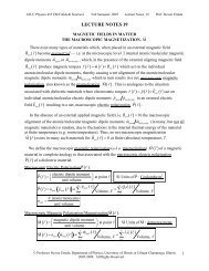
* Magnetism – arising from the motion of electric charges – the observer
is not in the same IRF as that of the moving charge – thus magnetism is
a consequence of the space-time nature of the universe that we live in
μ
(Lorentz contraction / time dilation and Lorentz invariance Δx Δ x = I ).
μ
B -gun
* “Magnetism” is not “just” associated with the phenomenon of electromagnetism, but ∀ four
fundamental forces of nature: EM, strong, weak and gravity (and anything else!) – because
space-time is the common “host” to all of the fundamental forces of nature – they all live /
exist / co-exist in space-time, and all are subject to the laws of space-time – i.e. relativity!
We can e.g. calculate the “magnetic” force between a current-carrying “wire” and a moving
(test) charge Q T without ever invoking laws of magnetism (e.g. the Lorentz force law, the Biot-
Savart law, or Maxwell’s equations (e.g. Ampere’s law)) – just need electrostatics and relativity!
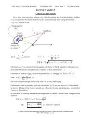
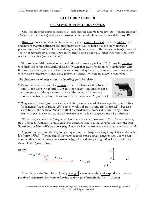
Suppose we have an infinitely long string of positive charges moving to right at speed v in the
lab frame, IRF(S). The spacing of the +ve charges is close enough together such that we can
consider them as continuous / macroscopic line charge density λ = q (Coulombs/meter) as
shown in the figure below:
IRF(S):
λ = q (> 0)
ˆx
I = λ v ϑ ẑ
v = vzˆ
ŷ
Since the positive line charge density λ = q is moving to right with speed v, we have a
positive filamentary / line current flowing to the right of magnitude I = λv
(Amps).
© Professor Steven Errede, Department of Physics, University of Illinois at Urbana-Champaign, Illinois
2005-2011. All Rights Reserved.
1

UIUC Physics 436 EM Fields & Sources II Fall Semester, 2011 Lect. Notes 18 Prof. Steven Errede
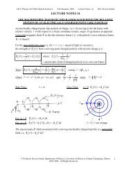
Now suppose we also have a point test charge Q T moving with velocity u =+ uzˆ
(i.e. to the
right) in IRF(S) {n.b. u = u is not necessarily = v = v}. The test charge Q T is a ⊥ distance ρ
from the moving line charge / current as shown in the figure below.
IRF(S):
λ = q (> 0)
ˆx
I = λ v ϑ ẑ
v = + vzˆ
ρ
ŷ
u = + uzˆ
Q T IRF(S') = rest frame of test charge
Let’s examine this situation as viewed by an observer in the rest frame of the test charge Q T
= the proper frame of the test charge Q T . Call this rest/proper frame = IRF(S').
By Einstein’s “ordinary” velocity addition rule, the speed of +ve charges in the right-moving
line charge density / filamentary line current as viewed by an observer in the rest frame IRF(S')
of the test charge Q T {which is moving with velocity u = + uzˆ
in the lab frame IRF(S)} is:
v−
u
v′ = with: v = + vzˆ
1 − vu
c
2
and:
u = + uzˆ
However, in IRF(S'), due to Lorentz contraction the {infinitesimal} spacing between positive
charges in the right-moving line charge / filamentary line current is also changed, which
therefore changes the line charge density as observed in IRF(S'), relative to the lab IRF(S)!
1 1
In IRF(S'): λ′ = γλ ′
0 where: γ ′ ≡ =
1− β′
1−
v′
c
( )
2 2
and: λ
0
= q
0 , λ′ = q ′
⇒ ′ =
0
γ ′
Where λ
0
= q
0 ≡ linear charge density as observed in its own rest frame IRF(S 0 ).
Once the line charge density λ
0
starts moving at speed v in IRF(S), then: → and 0
λ0
→ λ .
1 1
In IRF(S): λ = γλ0
where: γ ≡ =
1−
β 1−
vc
( )
2 2
and: λ
0
= q
0 , λ = q ⇒ =
0
γ
But:
∴
1
v−
u
γ ′ ≡
and: v′ = where: v = vzˆ
and: u = uzˆ
in IRF(S).
1−
( v′
c) 2 1 − vu
c
2
2
1 1
( c − vu)
γ ′ = = =
2 2 2
2
2
2 2
1 ( v−u) c ( v−u)
1 1
( c −vu) −c ( v−u
−
−
)
2
2
2
2
c ⎛ vu ⎞
1
( c − vu)
⎜ −
2 ⎟
⎝ c ⎠
2
© Professor Steven Errede, Department of Physics, University of Illinois at Urbana-Champaign, Illinois
2005-2011. All Rights Reserved.

UIUC Physics 436 EM Fields & Sources II Fall Semester, 2011 Lect. Notes 18 Prof. Steven Errede
Or:
⎛ uv ⎞
γ ≡
2
2
( c − uv
1
)
1
⎜ − ⎟
c
uv
γ′ ⎛ ⎞
= = i
⎝ ⎠
= γγ 1
2 2 2 2
2 2
u ⎜ −
2 ⎟ with:
( c −v ) −( c −u ) ⎛v⎞ ⎛u⎞
⎝ c ⎠
1−⎜ ⎟ 1−
γ
u
≡
⎜ ⎟
⎝c⎠ ⎝c⎠
1−
1
1−
( vc)
1
2
( uc)
2
Thus: γ uv
′ = γγ u ⎜
⎛ 1−
⎞
2 ⎟
⎝ c ⎠ with: v
= vzˆ
and:
u = uzˆ
Thus the line charge density λ′ as observed in the rest frame of the test charge Q T , i.e. in IRF(S') is:
λ′ ⎛
0
1 uv ⎞ ⎛
u 2 0 u
1 uv ⎞ ⎛
γλ γγ λ γ γλ
2 0
γu
1
uv ⎞
= ′ = ⎜ − ⎟ = ⎜ − ⎟ = ⎜ − λ
2 ⎟
⎝ c ⎠ ⎝ c ⎠ ⎝ c ⎠
Check: If u
= v
, does λ′ = λ ? 0
When u = v , the test charge QT is moving with the same velocity as the line charge, thus
the test charge Q T is in the rest frame of the line charge, i.e. IRF(S') coincides with IRF(S 0 )!
≡λ
If u
= v
then: u v
γ ≡
= and:
( ) 2
1
1−
vc
= γ
u
≡
1−
1
( uc) 2
Then:
⎡
2
⎛ u ⎞ ⎤
⎢
⎛ ⎞
1−
⎜ ⎟
⎥
⎜
uv
c ⎟
⎛ ⎞ ⎢ ⎝ ⎝ ⎠ ⎠ ⎥
λ′ = γγu
⎜1− λ
2 ⎟ 0
= ⎢ ⎥λ0 = λ0
⎝ c
2
⎠ ⎢ ⎛ ⎛u
⎞ ⎞ ⎥
⎢
1−
⎜ ⎜ ⎟
⎝c
⎠ ⎟ ⎥
⎢⎣
⎝ ⎠ ⎥⎦
YES! λ′ = λ0
.
Note that the line charge density λ as observed in the lab frame {i.e. in IRF(S)}, in terms of
the line charge density λ
0
in the rest frame of the line charge itself (i.e. IRF(S 0 )) is:
1
λ = γλ0 = λ
2
0
1−
vc
( )
since: γ ≡
1
( ) 2
1−
vc
Check: If u = 0 , does λ′ = λ ?
When u = 0 , the test charge Q T is not moving in the lab frame IRF(S), thus IRF(S')
coincides with IRF(S)!
If u = 0
then: u = 0 and:
1
γ
u
≡ = 1
1−
( uc) 2
⎡ uv ⎤
and thus: λ′ ⎛ ⎞
= ⎢γu
⎜1− λ = λ
2 ⎟
c
⎥ Yes!
⎣ ⎝ ⎠⎦
© Professor Steven Errede, Department of Physics, University of Illinois at Urbana-Champaign, Illinois
2005-2011. All Rights Reserved.
3

UIUC Physics 436 EM Fields & Sources II Fall Semester, 2011 Lect. Notes 18 Prof. Steven Errede
An observer in the proper / rest frame IRF(S') of the test charge Q T sees a radial ( ) ˆρ
electrostatic field in IRF(S') associated with the infinitely long line charge density
E′ =
λ′
⎡ uv ⎤
ρ with λ′ ⎛ ⎞
= γu
1 λ
2
πε ρ
⎢ ⎜ − ⎟
c
⎥ and λ = γλ0
⎣ ⎝ ⎠⎦
( ρ ) ˆ
2 o
n.b. ˆρ is the radial unit vector ⊥ to v = vzˆ
{and u = uzˆ
}.
⇒ ρ and ˆρ are unaltered / unaffected by Lorentz boosts along the ẑ -direction.
1 1 uv 1 uv
E ρ 1 1
2 2
2 λ ⎡
o
2 γ ⎤
o
c
λ ⎡
2
γ ⎤
′
⎛ ⎞ ⎛ ⎞
= ′ =
πε ρ πε ρ
⎢ ⎜ − ⎟⎥ = −
πε
oρ
⎢ ⎜ ⎟
c
⎥
⎣ ⎝ ⎠⎦ ⎣ ⎝ ⎠⎦
γ λ
∴ In IRF(S'): ( ) u
u
0
λ′ = q ′ of:
λ = q in IRF(S) λ0 ≡ q
0 in IRF(S 0 )
In the special case when u
= v
when IRF(S') ≡ IRF(S0 ) coincide → the test charge Q T and
the line charge λ0
are both at rest/in the same rest frame/same IRF:
1 1
Then: E′ ( ρ ) = λ′
= λ ≡ E ( ρ)
λ = q
u v
0 0 ← Purely electrostatic field,
=
0 0
2πε oρ
2πε oρ
n.b. Notice that when IRF(S') ≡ IRF(S 0 ) coincide, that F0 = QT
E0
⊥ ( u = v)
:
QT
Q ⎛
T
q ⎞
q
F0( ρ ) = Q
0( ) ˆ
ˆ
T
E ρ = λ0ρ = ⎜ ⎟ρ
where: λ
0
=
2πε oρ
2πε oρ
⎝
0 ⎠
0
For the more general case where u ≠ v , the force acting on the test charge QT in its own rest
frame IRF(S') is:
But: I
QT
QT
⎡ uv ⎤
F′ ⎛ ⎞
TOT ( ρ ) = QT E′ TOT ( ρ) = λ′
= γu
1 λ
2
2πε oρ
2πε oρ
⎢ ⎜ − ⎟
c
⎥ where:
⎣ ⎝ ⎠⎦
Q Q uv
F′ ⎛ ⎞
ρ = γ λ − γ λ⎜ ⎟
T
T
Or: TOT ( ) u u 2
2πε ρ 2πε ρ ⎝c
⎠ where: u
( ) 2
Or: F ( ρ )
o
o
γ ≡
QT
λ λv
⎛ 1 ⎞ QTu
′ = − ⎜ ⎟
2πε oρ 1−
2πε c ρ 1
TOT
≡ λv
in IRF(S) {the lab frame} and
2
( uc) o ⎝ ⎠ −( uc)
2 2
2
1 c ε
oμo
= :
1
1−
uc
q
λ =
In IRF(S)
Thus: F ( ρ )
QT
λ ⎛ μoI
⎞ QTu
′ = − ⎜ ⎟
2πε oρ
1−
2πρ
1
TOT
( uc) ⎝ ⎠ −( uc)
2 2
in IRF(S')
Or: F′ ( ρ ) = Q E′ ( ρ) − Q uB′ ( ρ) = Q E′
( ρ)
and: E′ ( ρ ) = E′ ( ρ) − uB′
( ρ)
TOT T T T TOT
TOT
4
© Professor Steven Errede, Department of Physics, University of Illinois at Urbana-Champaign, Illinois
2005-2011. All Rights Reserved.

UIUC Physics 436 EM Fields & Sources II Fall Semester, 2011 Lect. Notes 18 Prof. Steven Errede
1 λ
⎛ μo
⎞ I
Where: E′ ( ρ ) =
and: B′ ( ρ ) = ⎜ ⎟
in IRF(S') !!!
2πε oρ
1−
( uc) 2
⎝2πρ
⎠ 1−
( uc) 2
Vectorially, in the general IRF(S') / rest frame of the test charge Q T , for u ≠ v {necessarily}
F′ TOT ( ρ ) = QT E′
TOT ( ρ ) ← n.b. in the radial / ˆρ direction only.
Very Useful Table
∴ F′ ( ) ( ) ˆ ( ) ˆ
TOT
ρ = QT E′ ρ ρ−QT
uB′
ρ ρ
Cylindrical Coordinates:
ˆ ρ × ˆ ϕ = zˆ
ˆ ϕ× ˆ ρ =−zˆ
But: u = uzˆ
∴ u× B′ ( ρ ) =−uB′
( ρ) ˆ ρ ⇒ B′ = B′
ˆ ϕ then: uB′ ( zˆ
× ˆ ϕ ) =−uB′
ˆ ρ ˆ ϕ × zˆ
= ˆ ρ zˆ× ˆ ϕ =− ˆ ρ
=− ˆ ρ
zˆ× ˆ ρ = ˆ ϕ ˆ ρ× zˆ
=−ˆ
ϕ
F′ TOT ( ρ ) = QT E′ TOT ( ρ) = QT E′ ( ρ) + QT
( u×
B′
( ρ)
) ← Lorentz Force Law in IRF(S') !!!
1 λ ⎛ μo
⎞ I
E′ ( ρ ) =
ˆ ρ B′ ( ρ)
= ⎜ ⎟
ˆ ϕ
2πε oρ
1−
( uc) 2
⎝2πρ
⎠ 1−
( uc) 2
Where:
in IRF(S')
γλ
u
γγλ
u 0
= ˆ ρ = ˆ ρ
⎛ μo
⎞ ⎛ μo
⎞
= γ ˆ
ˆ
uIϕ = γγuI0ϕ
2πεoρ
2περ
⎜ ⎟ ⎜ ⎟
o
⎝2πρ
⎠ ⎝2πρ
⎠
I
≡ = = I′ ≡ γ
uλv= γγuλ0v=
γγuI0
0
≡ λ0v
I λv γλ0v γ I0
I′ = γ
uI
ẑ in IRF(S')
ρ Q B′
( ρ ) ˆ ϕ
T
u = uzˆ
QT
λ
⎛ μoI
⎞ 1
F′ ( )
ˆ
ˆ
TOT
ρ = ρ − Q
2
2
Tu⎜ ⎟ ρ
πε
2
oρ
1−( uc) ⎝2πρ
⎠ 1−( uc)
in IRF(S')
= QE′ T ( ρ) + Qu
T
× B′
( ρ)
repulsive
force
attractive
force
For like charges q = λ and Q T If u || v
{remember: I = λv
}
Next, we Lorentz transform the IRF(S') results (defined in the rest / proper frame of Q T )
to the IRF(S) (lab frame), using the rule(s) for Lorentz transformation of forces:
1 λ
λv
I
E
2πε
oc
ρ 1−
F Q E Q E Q u B
′( ρ ) =
ˆ ρ and: B′ ( ρ ) =
2πε oρ
1−
( uc) 2
′ ( ρ ) = ′ ( ρ) = ′( ρ) + × ′( ρ)
TOT T TOT T T
in IRF(S)
n.b. Parallel currents attract
each other!!! {2 nd current is
test charge Q T !!!}
( uc)
2 2
QT
QT
⎡ uv ⎤
F′ ( ) ˆ
⎛ ⎞
1 ˆ
TOT
ρ = λρ ′ = γu
⎜ − λρ
2 ⎟
2πε oρ
2πε oρ
⎢
c
⎥ where: γ
u
=
⎣ ⎝ ⎠⎦
The test charge Q T is moving with velocity u = uzˆ
in the lab frame, IRF(S).
ˆ ϕ
1−
1
( uc) 2
© Professor Steven Errede, Department of Physics, University of Illinois at Urbana-Champaign, Illinois
2005-2011. All Rights Reserved.
5

UIUC Physics 436 EM Fields & Sources II Fall Semester, 2011 Lect. Notes 18 Prof. Steven Errede
Note that {here}: u = uzˆ = u zˆ
z
{i.e.
u = u , u zˆ
}, note also that: F
′
TOT
⊥ u
and F′ = F 0 z
′ =
z
.
Then the Lorentz transformation of the forces from IRF(S') to IRF(S):
F 1 F′ ⊥ ⊥
1 u c F′
⊥
γ ′
In IRF(S): = = −( ) 2
∴ In IRF(S):
Again:
F
TOT
u
( ) F ( )
where:
γ ′ ≡
u
1−
1
( uc) 2
and: F = F′
(= 0)
1 1 QT
1 QT
⎡
ρ ′ ˆ
TOT
ρ ρλρ ′
⎛ uv ⎞⎤
= = =
γ
u
1 ˆ
2
γu γu 2πεo γ
u
2πε oρ
⎢ ⎜ − ⎟
c
⎥λρ
⎣ ⎝ ⎠⎦
QT ⎛ uv ⎞ QTλ
QTλv
1
= ⎜1− ˆ ˆ u ˆ but: I v and
2 ⎟λρ = ρ − ∗ ρ ≡ λ = ε
2 2 oμo
2πε oρ ⎝ c ⎠ 2πε oρ 2πε
oc c
⎛ λ ⎞ ⎛ μoI
⎞
= Q ˆ
ˆ
T ⎜ ρ⎟ − QT
⎜u∗
ρ⎟
⎝2πε oρ
⎠ ⎝ 2πρ
⎠
u = uzˆ
, ẑ ˆ ϕ ˆ ρ
B
μ I o
ρ = ϕ
2πρ
× =− thus: ( ) ˆ
Note the cancellation of γ
u
factors !!!
∴ In IRF(S): ( )
⎛ λ ⎞ ⎛ μoI
⎞
F ˆ
ˆ
TOT
ρ = QT ⎜ ρ⎟ + QT
u×
⎜ ϕ⎟
⎝2πε oρ
⎠ ⎝2πρ
⎠
≡E
( ρ ) ≡B( ρ )
F Q E Q E Q u B
( ρ ) = ( ρ) = ( ρ) + × ( ρ)
TOT T TOT T T
← Lorentz Force Law in IRF(S) !!!
In IRF(S): E ( )
B
( q )
λ
ρ = ˆ ρ = ˆ ρ
2πε ρ 2περ
( )
o
o
( )
μoI
μoλv
μo
q v
ρ = ˆ ϕ = ˆ ϕ = ˆ ϕ
2πρ 2πρ 2πρ
where: λ = q = γλ = γ ( q )
0 0
where: I = λv= ( q ) v = γλ = γ ( )
v q v
0 0
Thus, an observer at rest in either the lab frame IRF(S) or the rest frame of the test charge IRF(S')
will see both a static electric field {different in each IRF} and a static (but velocity-dependent)
magnetic field {different in each IRF} due to the {infinitely long} filamentary line charge density
λ = q that is moving with velocity v = vzˆ
in IRF(S) = filamentary line current I = λv
in IRF(S).
The magnetic field arises simply from the relativistic effect(s) of electric charge in {relative} motion!
For an observer in the rest frame IRF(S 0 ) of the filamentary line charge density
see only a static, radial electric field!
λ = q
, he/she will
6
© Professor Steven Errede, Department of Physics, University of Illinois at Urbana-Champaign, Illinois
2005-2011. All Rights Reserved.

UIUC Physics 436 EM Fields & Sources II Fall Semester, 2011 Lect. Notes 18 Prof. Steven Errede
Let’s summarize these results by inertial reference frame:
IRF(S) IRF(S') IRF(S 0 )
Laboratory Frame Rest Frame of Test Charge Rest Frame of Line Charge
Moving with u = uzˆ = u zˆ
in lab
Moving with v = vzˆ = v zˆ
z
z
in lab
v−
u
v′ =
1 −
2
( uv c )
Speed of line
charge in IRF(S')
γ =
1
( ) 2
1−
vc
γ uv
′ = γγ ⎛ u ⎜1−
⎞
2 ⎟ γ
u
=
c
⎝ ⎠ ( ) 2
1
1−
uc
( q )
0
0
q
0 u
1
2 0 0
q
0
λ = q = γλ = γ
⎡ uv ⎤
λ′ ⎛ ⎞
= ′ = γλ ′ = γγ ⎢ − ⎜ ⎟ λ
c ⎥
⎣ ⎝ ⎠⎦
λ =
uv
=
0
γ
′ = 0 γ′
=
0
γγ ⎡ u ⎢1
− ⎛ ⎞⎤
⎜ 2 ⎟
c
⎥
0
⎣ ⎝ ⎠⎦
E
λ γλ
ρ ρ ˆ ρ
2πε ρ 2περ
0
( ) = ˆ =
I λv γλ v γ I
B
o
o
λ
γ
uλ
γγuλ0
E′ ( ρ ) = ˆ ρ = ˆ ρ
2πε ρ 2περ
≡ =
0
=
0
I0 ≡
0v
I
u
v
uI u 0v uI0
μ I μγI
ρ ϕ ˆ ϕ
2πρ
2πρ
o
o 0
( ) = ˆ =
F = Q E + Q u×
B
TOT T T
o
o
E
λ
0
( ρ ) =
ρ
ˆ
0
2πε o
ρ
′ ≡ γ λ = γ = γγ λ = γγ No current in IRF(S 0 )
μoI′
μγ
o uI μγγ
o uI0
B′ ( ρ ) = ˆ ϕ = ˆ ϕ = ˆ ϕ No B-field in IRF(S 0 )
2πρ 2πρ 2πρ
F′ = Q E′ + Q u×
B′
≠ TOT T T
≠ F′ ( ρ ) = Q E ( ρ )
0TOT
T 0
n.b. In the rest
frame IRF(S') of
the test charge Q T ,
the Lorentz force
F′ uses the
TOT
velocity u of the
test charge as
observed in the lab
frame IRF(S).
We see that the observed line charge densities λ and λ′ as seen in the lab frame IRF(S) and
the test charge rest frame IRF(S'), respectively are larger by factors of γ and γ ′ respectively
compared to the line charge density as observed in the rest frame IRF(S 0 ) of the line charge
density itself. This difference arises due to the effect of the {longitudinal} Lorentz contraction of
the moving line charge densityλ 0
, as viewed from the lab frame IRF(S) and the rest frame
IRF(S') of the test charge, respectively.
Because of this, the electric fields as seen in the lab frame IRF(S) and rest frame of the test
charge IRF(S') are larger by factors of γ and γγ
u
, respectively than that observed in the rest
frame IRF(S 0 ) of the line charge density itself, hence the magnitude of the electrostatic forces are
larger by these same amounts in their respective IRF’s, and are thus {in general} not equal.
An important point here is that in all 3 inertial reference frames, what we call the electric field
in each IRF is such that a.) they are all oriented in the same direction {here, the radial direction
and b.) they all have the same functional dependence (here, ~1 ρ ), differing only by γ -factors
from each other.
© Professor Steven Errede, Department of Physics, University of Illinois at Urbana-Champaign, Illinois
2005-2011. All Rights Reserved.
7

UIUC Physics 436 EM Fields & Sources II Fall Semester, 2011 Lect. Notes 18 Prof. Steven Errede
In the rest frame IRF(S 0 ) of the line charge density λ
0
the electromagnetic field seen there is
purely electrostatic, oriented in the radial ( ˆρ ) direction, whereas in the lab frame IRF(S) and the
rest frame of the test charge IRF(S'), the electromagnetic field observed in each of these two
reference frames is a combination of a static, radial electric field and a static, azimuthal magnetic
field.
The “appearance” of azimuthal magnetic fields in the lab frame IRF(S) and the rest frame of
the test charge IRF(S') is due to the relativistic effects associated with the motion of the line
charge density relative to an observer in the lab frame IRF(S) and/or the rest frame of the test
charge, IRF(S').
We say that the relative motion of the electric line charge density λ = γλ0
{as viewed by an
observer in the lab frame IRF(S)} constitutes an electric current I ≡ λv= γλ0v
{as viewed by that
same observer in the lab frame IRF(S)}.
We then connect / associate the “appearance” of azimuthal magnetic fields B
and B′ in the
lab frame IRF(S) and the rest frame of the test charge IRF(S'), respectively with the existence of
the electric currents I and I′ as observed in their respective inertial reference frames.
The B -field in each IRF is linearly proportional to {the magnitude of} the electric current | I | as
observed in that IRF, i.e. | B |~| I | = | λv
| .
Another interesting/important aspect of the magnetic fields B that “appear” in IRF(S) and/or
IRF(S') is that they are mutually ⊥ to both E
.and. I = λv
in that IRF.
Note that we could instead refer to electric currents I alternatively and equivalently,
exclusively and explicitly as to what they are truly are – the {relative} motion(s) of charges qv ,
line charge densities λv
, surface charge densitiesσ v
and/or volume charge densities ρv
.
Then we also wouldn’t have to explicitly use the descriptor “magnetic” field to describe the
resulting component of the electromagnetic field that does arise from the relative motion(s) of
electric charge(s) as viewed by an observer who is not in the rest frame of these electric
charge(s). We could call it something else instead – e.g. “the relativity field”.
We humans call this field “the magnetic field” largely for historical inertia reasons. Magnetic
fields were discovered centuries before relativity and space-time were finally understood; thus
we simply keep calling this field “the magnetic field”. The magnetic field is truly and simply one
component of the overall electromagnetic field that is associated with a physical situation, and
one which only arises whenever that physical situation is viewed by an observer whose IRF(S) is
not coincident with the rest frame IRF(S 0 ) of the electric charge(s) that are present in that
particular physical situation.
The “traditional” way of equivalently saying the above is: “Magnetic fields are only produced
when electrical currents are present”.
8
© Professor Steven Errede, Department of Physics, University of Illinois at Urbana-Champaign, Illinois
2005-2011. All Rights Reserved.

UIUC Physics 436 EM Fields & Sources II Fall Semester, 2011 Lect. Notes 18 Prof. Steven Errede
Physical Electric Currents:
It is important to understand that there exist different kinds of physical electric currents.
• A “bare” filamentary line charge density λ = q e.g. moving with uniform velocity v = vzˆ
with respect to the lab frame IRF(S), creates a filamentary line current I = λvzˆ
in the lab
frame IRF(S). This filamentary line current is not equivalent to a physical electrical current
flowing e.g. in an “infinitesimally-thin” physical wire at rest in the lab frame IRF(S). For an
observer in {any} IRF the “bare” filamentary line charge density has a net / overall electric
charge. An observer at rest in the lab frame IRF(S) sees both a static, non-zero radial electric
field and a static, non-zero azimuthal magnetic field arising from the “bare” filamentary line
charge density λ = q and “bare” filamentary line current I = λvzˆ
respectively, whereas an
observer at rest in IRF(S 0 ) of the filamentary line charge density λ
0
= q
0
sees no magnetic
field – only a static, radial electric field!
• In a physical wire (e.g. a copper wire, made up of copper atoms with “free” conduction
electrons), the “free” negatively-charged electrons move / drift through the macroscopic
volume of the copper wire e.g. with {mean} drift velocity v ˆ
D
= −vDz
and constitute a
wire
wire
physical electric current I J
A
n ev
= A
−i =− − i as viewed by an observer in the lab
phys
e
⊥
e
frame IRF(S). Microscopically, the copper wire is a 3-D “matrix” (or lattice) of bound / fixed
copper atoms with a “gas” of “free” conduction electrons drifting through it. In the lab frame
IRF(S), the copper atoms are at rest. Note importantly {also} that in the lab IRF(S), the
physical current-carrying copper wire has no net electric charge – because there is one “free”
conduction electron associated with each copper atom of the copper wire. Thus, an observer
at rest in the lab frame IRF(S) sees no net electric field but does see a static, non-zero
azimuthal magnetic field arising from the “free” conduction electron volume current density
J − =−n −ev
e e D , whereas an observer at rest in IRF(S0 ) “free” conduction electron charge
0 0
density ρ n e
e − =
e − sees no magnetic field associated with the “free” conduction electrons, but
does see {the same!} non-zero azimuthal magnetic field that is associated with volume
current density JCu =+ nCuevD
of the 3-D lattice of copper atoms that are moving with
{relative} velocity v =+ v zˆ
to an observer at rest in IRF(S 0 ) !!!
D
D
• In semiconducting materials (e.g. silicon, germanium, graphite, diamond, SiC, gallium, …)
electrical conduction occurs either by mobile “drift” electrons and/or “holes” {= the absence
of an electron). The number densities of electrons and/or “holes” are both typically
number density of semiconductor atoms and depend on details associated with the
condensed matter physics of the semiconductor. In general n − ≠ n
e hole
and both are strong
(exponential) functions of {absolute} temperature. The drift velocities of electrons and holes
are not in general the same. Thus, in the lab frame IRF(S), an observer will, in general see
static electric field contributions arising from both electron and hole charge density
distributions as well as magnetic field contributions from both electron and hole current
densities. An observer at rest either in IRF(S 0 ) of the electrons or at rest IRF(S * 0 ) of the holes
will again see static electric field contributions from both electrons and holes, but a B-field
contribution only from holes (electrons), respectively.
D
⊥
© Professor Steven Errede, Department of Physics, University of Illinois at Urbana-Champaign, Illinois
2005-2011. All Rights Reserved.
9

UIUC Physics 436 EM Fields & Sources II Fall Semester, 2011 Lect. Notes 18 Prof. Steven Errede
• The situation of a “bare” filamentary line charge λ = q moving with {relative} velocity
v = vzˆ
in IRF(S), producing a filamentary line current I = λv
in IRF(S) can be physically
realised e.g. as “beam” of +ve current of protons (+q) {or e.g. +ve ions, or e.g. –ve electrons}
flowing in a vacuum (e.g. made via laser photo-ionized hydrogen, argon, or thermionic
emission of electrons, respectively):
Vacuum Chamber (Lab IRF(S))
→
v = vzˆ
Protons/ions moving with constant velocity
v = vzˆ
in drift region.
Protons/ions accelerated here, gain kinetic
2
energy E = eΔ V = ( γ − 1) m c
kin
e
Having discussed the EM field(s) and EM force(s) acting on a test charge Q T associated with a
single filamentary line charge / filamentary line current as observed in different IRF’s, we now
discuss the problem of two counter-moving, opposite-charged filamentary line charges /
filamentary line currents superimposed on top of each other.
Consider two opposite-charged filamentary line charges (both infinitely long) that are initially
stationary in the lab frame IRF(S). One initially stationary filamentary line charge has negative
charge per unit length λ0 −
≡−q
0 and the other initially stationary filamentary line charge has
positive charge per unit length λ
0 +
=+ q
0 . The two line charges are then set in motion parallel
to / along their axes (in the ẑ -direction). The negative line charge moves to the left
( −ẑ
direction) with velocity v =− vzˆ
− in the lab frame IRF(S), and the positive line charge moves
to the right (+ ẑ direction) with velocity v = + vzˆ
+ in the lab frame IRF(S) {i.e. it has the same
exact speed, but moves in the opposite direction to that of the first line charge}.
The two counter-moving filamentary line charges are superimposed on top of each other /
coaxial with each other, but we draw them as slightly displaced (transverse to their motion) for
clarity’s sake in the figure below, as seen by an observer at rest in the lab IRF(S):
ˆx
In IRF(S): v =− vzˆ
−
λ −
= − q IRF(S)
ϑ ẑ
λ +
=+ q v = + vzˆ
+
ŷ
In IRF(S), the moving filamentary line charges have charge per unit length λ ±
=± q , whereas
in the respective rest frame(s) IRF(S ± ) of the filamentary line charges, we have λ0 =± q 0
≡± λ . 0
±
10
© Professor Steven Errede, Department of Physics, University of Illinois at Urbana-Champaign, Illinois
2005-2011. All Rights Reserved.

UIUC Physics 436 EM Fields & Sources II Fall Semester, 2011 Lect. Notes 18 Prof. Steven Errede
Because of the respective motions of the line charge densities:
Then: λ γλ0
1 1
γ = =
=± where: ±
1−( v c) 1−( v c)
±
2 2
v = ± vzˆ
±
In the lab frame IRF(S): A negative current I
positive current I
= λ v flowing to the left is superimposed on a
− − −
= λ v flowing to the right, as shown in the figure below:
+ + +
In IRF(S): I− = λ−v
ˆ
−
v =− −
vz
ˆx
I
= λ v v =+ vzˆ
+
+ + +
ŷ
ϑ
ẑ
Using the principle of linear superposition, the net/total current {as observed in the lab frame
IRF(S)} is:
I = I + I = λ v + λ v but: λ = − λ and: v = − v
TOT
+ − + + − −
− +
∴ ( )( ) 2
TOT
− +
I = λ v + −λ − v = λ v + λ v = λ v flowing to the right (i.e. in + ẑ direction)
+ + + + + + + + + +
⇒ ITOT
= 2λ+ v+
= 2λv
flowing in the ẑ -direction: with: λ ≡ + +
λ =+ q , v
=+ vzˆ
+
ẑ and: λ ≡ − −
λ =− q , v
=−vzˆ
−
Note that because we have superimposed these two counter-moving, filamentary oppositelycharged
line-charges / counter-moving, filamentary line currents, the net electric charge Q TOT
{as observed in the lab frame IRF(S)} is zero because:
λ = λ + λ =+ λ− λ = 0 in the lab frame IRF(S).
TOT
+ −
If Q TOT = 0 in IRF(S), then we also know that the net electric field ETOT
( r ) = 0 in the lab
frame IRF(S) due to these two counter-moving, superimposed oppositely-charged filamentary
line charges/line currents in IRF(S).
Now additionally suppose that we also have a test charge Q T moving with velocity u = uzˆ
(i.e. to the right) in IRF(S). As before, u
is not necessarily = v = vzˆ
, the velocity of right
moving line charge. The test charge Q T is a ⊥ distance ρ from the superimposed oppositecharged,
opposite-moving filamentary line charges λ+ and λ : −
ˆx
In IRF(S): λ −
=−q
v =− vzˆ
−
I− = λ−v−
IRF(S)
ITOT
= 2λv
ϑ ẑ
λ +
=+ q v =+ vzˆ
+
I+ = λ+ v+
ŷ
ρ
u = + uzˆ
Q T
© Professor Steven Errede, Department of Physics, University of Illinois at Urbana-Champaign, Illinois
2005-2011. All Rights Reserved.
11

UIUC Physics 436 EM Fields & Sources II Fall Semester, 2011 Lect. Notes 18 Prof. Steven Errede
Let’s examine the situation as viewed by an observer in IRF(S') – i.e. the rest frame of the test
charge Q T . There are four distinct cases to consider for the 1-D Einstein velocity addition rule:
a.) In the lab frame IRF(S), the test charge Q T is moving with velocity u =+ uzˆ
,
the +ve filamentary line charge density λ = + λ is moving with velocity v
=+ vz ˆ
+ .
+
Lab Frame IRF(S):
ˆx
ẑ
ŷ ϑ
λ+ =+ λ =+ q v
= + vz ˆ
+ v−
u
ẑ
v′ +
= =
vu
ρ
1−
2
c
u = + uzˆ
Q IRF( S′ ) = rest frame of test charge
T
b.) In the lab frame IRF(S), the test charge Q T is moving with velocity u =+ uzˆ
,
the −ve filamentary line charge density λ = −λ
is moving with velocity v
=−vz
ˆ
− .
−
Relative
speed of +λ
viewed from
IRF(S')
ŷ
ŷ
Lab Frame IRF(S):
ϑ
ˆx
ẑ
−v−
u
v′ −
=
vu
1+
2
c
c.) In the lab frame IRF(S), the test charge Q T is moving with velocity u =−uzˆ
,
the +ve filamentary line charge density λ = + λ is moving with velocity v
=+ vz ˆ
+ .
Lab Frame IRF(S):
ϑ
ˆx
ẑ
λ− =− λ =−q
v
= −vz
ˆ
−
ρ
u = + uzˆ
Q IRF( S′ ) = rest frame of test charge
T
λ+ =+ λ =+ q v
= + vz ˆ
+
+
ρ
u = −uzˆ
Q IRF( S′ ) = rest frame of test charge
T
v+
u
v′ +
=
vu
1+
2
c
d.) In the lab frame IRF(S), the test charge Q T is moving with velocity u =−uzˆ
,
the −ve filamentary line charge density λ = −λ
is moving with velocity v
=−vz
ˆ
− .
−
ẑ
ẑ
=
=
Relative
speed of −λ
viewed from
IRF(S')
n.b. only v reversed
relative to case a.) above
Relative
speed of +λ
viewed from
IRF(S')
n.b. only u reversed
relative to case a.) above
Lab Frame IRF(S):
ˆx
ẑ
ŷ ϑ
λ− =− λ =−q
v
= −vz
ˆ
−
ẑ
ρ
u = −uzˆ
Q IRF( S′ ) = rest frame of test charge
T
− v+
u
v′ −
=
vu
1−
2
c
=
Relative
speed of −λ
viewed from
IRF(S')
n.b. both u and v reversed
relative to case a.) above
12
© Professor Steven Errede, Department of Physics, University of Illinois at Urbana-Champaign, Illinois
2005-2011. All Rights Reserved.

UIUC Physics 436 EM Fields & Sources II Fall Semester, 2011 Lect. Notes 18 Prof. Steven Errede
The above four relative 1-D speed formulae can be more compactly written as two specific cases:
i.) For
ii.) For
u =+ uzˆ
:
u =−uzˆ
:
± v−
u
v′ ±
=
vu
1
c
± v+
u
v′ ±
=
vu
1
c
v u
v ′ = ∓
±
vu
1∓
c
1-D general:
v−
u
v′ =
vu i
1−
c
∓
2
2
±
2 the u = −uzˆ
case. Then his formula agrees
2
Thus, for an observer in IRF(S') (= rest frame of Q T ) moving to the right with velocity
in IRF(S) we see that v′ > v′
.
− +
u = + uzˆ
Because v′ −
> v′
+ for an observer in IRF(S'), the Lorentz contraction of the –ve filamentary line
charge density λ −
=−q
will be more “severe” than that associated with the +ve filamentary
line charge density λ +
=+ q .
1
In IRF(S'): λ′ ±
=± γλ ′
± 0 where: γ ±
′ ≡
1−
( v′
c) 2
±
And: ± λ0 = q
0 = filamentary line charge densities in their own rest frames.
± v−u
v =+ vzˆ
But: v′ ±
= for:
vu
in IRF(S)
1∓
u =+ uzˆ
2
c
Thus:
1 1 1
′ = = = =
2
( c ∓ vu)
2
( c ∓ vu)
( ∓ ) ( )
γ ±
2 2 2 2
2
2
2
2
⎛v′ ± ⎞ 1 ( ± v− u) c ( ± v−u)
1− c vu − c ± v−u
⎜ ⎟ 1− 1−
2
2
2
2
⎝ c ⎠ c ⎛ vu ⎞
1∓
( c ∓ vu)
2
⎜
⎝
n.b. Equation 12.76, p. 523 in Griffith’s
book is correct, however the proper use of
his equation explicitly requires placing a
− (minus) sign in front of the formula for
the v −
′ case. Note that (obviously) u must
also be explicitly signed in his formula for
with the 4 that are explicitly given here.
c
⎟
⎠
( )
2
c ∓ vu
=
=
4
2 2 2 2
2 2 4 2 2 2 2
c ∓ 2vuc
+ ( vu)
− c v ± 2vuc
− cu c −c v − c u + vu
⎛ vu ⎞
2
1
2
( c ∓ vu)
1
⎜ ∓ ⎟
c ⎛ uv ⎞
= = i
⎝ ⎠
= γγ 1
2 2 2 2
2 2
u ⎜ ∓
2 ⎟
( c −v )( c −u ) ⎛v⎞ ⎛u⎞
⎝ c ⎠
1−⎜ ⎟ 1−⎜ ⎟
⎝c⎠ ⎝c⎠
( )
2 2
uv
Or: γ′ ⎛ ⎞
±
= γγu
⎜1∓ 2 ⎟ where: γ ≡
⎝ c ⎠
1
⎛v
⎞
1− ⎜ ⎟
⎝c
⎠
2
and: γ
u
≡
1
⎛u
⎞
1− ⎜ ⎟
⎝c
⎠
2
© Professor Steven Errede, Department of Physics, University of Illinois at Urbana-Champaign, Illinois
2005-2011. All Rights Reserved.
13

UIUC Physics 436 EM Fields & Sources II Fall Semester, 2011 Lect. Notes 18 Prof. Steven Errede
⎛
0 0
1 uv ⎞ ⎛
u 2 u 0
1 uv ⎞ ⎛
1
uv ⎞
λ± =± γ±
λ =± γγ λ ⎜ ⎟=± γ γλ ⎜ γ
2 ⎟=±
uλ⎜ 2 ⎟
⎝ ∓ c ⎠ ⎝ ∓ c ⎠ ⎝ ∓ c ⎠
Then in IRF(S'): ′ ′
( )
where: γ =
u
1−
1
( uc) 2
and: γ ≡
1
( ) 2
1−
vc
But: ± λ =± γλ0
= charge per unit length in the lab frame, IRF(S).
∴In IRF(S'):
⎡
uv
⎤
⎢ ⎛ ⎞
1
2
uv
⎜ − ⎟
⎥
c
λ′ ⎛ ⎞ ⎢ ⎥
+
=+ γuλ 1 λ
⎝ ⎠
⎜ −
2 ⎟=
c
2
⎝ ⎠
⎢ ⎥
⎢ ⎛u
⎞
1− ⎥
⎢ ⎜ ⎟
⎣ ⎝c
⎠ ⎥
⎦
and:
⎡
uv
⎤
⎢ ⎛ ⎞
1
2
uv
⎜ + ⎟
⎥
c
λ′ ⎛ ⎞ ⎢ ⎥
−
=− γuλ 1 λ
⎝ ⎠
⎜ +
2 ⎟=−
c
2
⎝ ⎠
⎢ ⎥
⎢ ⎛u
⎞
1− ⎥
⎢ ⎜ ⎟
⎣ ⎝c
⎠ ⎥
⎦
In IRF(S'):
ˆx
v ′ =− vz ′ ˆ
−
I′ −
= λ′ −v′
−
λ −
′ = − q ′
IRF(S')
I′ TOT
= 2λ′′
v ϑ ẑ
λ +
′ =+ q ′ I′ +
= λ′ +
v′
ˆ
+
v ′ = + +
vz ′
ŷ
ρ
u = + uzˆ
{in lab frame IRF(S)}
Q T
At rest in IRF(S')
∴ In the rest frame IRF(S') of the test charge Q T , the total/net line charge density is: λ′ TOT
= λ′ +
+ λ′
− .
In IRF(S'): λ 1 uv uv
′ λ ′ λ ′ γ λ ⎛ ⎞
TOT u
1
2 u 2 u
c
γ λ ⎛ ⎞
c
γ λ ⎛uv
⎞
uv
=
+
+
−
= ⎜ − ⎟− ⎜ + ⎟=
−γλ
u ⎜ 2 ⎟−
γλ
u
−γλ ⎛
u ⎜ ⎞
2 ⎟
⎝ ⎠ ⎝ ⎠
⎝c
⎠
⎝c
⎠
2
uv ( uv c )
λ′ ⎛ ⎞
TOT
=− 2γuλ⎜
2λ
0!!!
2 ⎟=− ≠
c
2
⎝ ⎠ 1−
uc
( )
⇒ In IRF(S') {= rest frame of the test charge Q T (which moves with velocity u = uzˆ
in IRF(S))}
2
( uv / c )
∃ a net –ve line charge density λ′ TOT
=−2λ
!!!
2
1−
( uc)
Whereas in the lab frame IRF(S), ∃ no net line charge, i.e. λ
TOT
= 0 in IRF(S) !!!
⇒ The non-zero λ′
TOT
observed in IRF(S') (= rest frame of Q T ) is due to / arises from the
unequal Lorentz contraction of the +ve vs. –ve filamentary line charge densities, as observed
in IRF(S') (= rest frame of Q T ).
⇒ A current-carrying “wire” that is electrically neutral ( λ
TOT
= 0) in one IRF(S) will NOT be so
in another IRF(S') !!! It will have a net electrical charge in IRF(S') ≠ IRF(S) !!!
14
© Professor Steven Errede, Department of Physics, University of Illinois at Urbana-Champaign, Illinois
2005-2011. All Rights Reserved.

UIUC Physics 436 EM Fields & Sources II Fall Semester, 2011 Lect. Notes 18 Prof. Steven Errede
Thus in IRF(S'), where there exists a net –ve line charge density of:
a corresponding (radial-inward) electric field exists: E ( )
λ′ =−2λ
TOT
2
( uv / c )
1−
( uc)
2
( uv / c )
λ′
TOT
λ
′ ρ = ˆ ρ =−
ˆ ρ .
2πε 2
oρ
πε
oρ
1−
( uc)
Thus an observer in the rest frame IRF(S') of the test charge Q T “sees” a radial-inward (i.e.
attractive) electrostatic force acting on the test charge Q T (for Q T > 0) of:
But: E ( ρ)
TOT
F ( ρ ) Q ( ) ˆ
TE ρ Q λ ′
′ = ′ =
T
ρ
2πε ρ
2
λ′
2λ
( uv / c )
TOT
′ = ˆ ρ =−
2πε ρ 2πε ρ
o
o
o
( uc)
2
( uv / c )
1 λ
1
ˆ ρ =−
1−
πε ρ 1−
( uc)
2 2
o
n.b. Lorentz-invariant !!!
Valid in any/all IRF’s
ˆ ρ
2
1
and:
2
c
= ε μ
o
o
∴ E ( ρ )
λεo
μ0
′ =−
uv
ρ
1
μλ
o
v u
ˆ ρ =−
πρ
πε
2 2
o 1−( uc) 1−( uc)
ˆ ρ
But: I = 2λv
in lab IRF(S).
∴ In IRF(S') (= rest frame of Q T ): E ( ρ )
μ I u
o
′ =−
2πρ
1−
Therefore equivalently, the force F′ ( ρ ) = Q E′
( ρ )
μoQI
T
u
F′ ( ρ ) = QT
E′
( ρ)
=−
ρ
2πρ
1−
T
ˆ
( uc) 2
ˆ
( uc) 2
ρ ⇐ n.b. points radially inward!
acting on Q T in its own rest frame IRF(S') is:
This force is none other than the magnetic Lorentz force acting on Q T :
In IRF(S') (= rest frame of Q T ): F′ ( ρ ) = QT
( u×
B′
( ρ )
Where
)
u = + uzˆ
= velocity of
test charge Q T in IRF(S)
E′ ( ρ ) = u×
B′
( ρ ) μoI
1
μoI
1
B′ ( ρ ) = ˆ ϕ = γ ˆ
u
ϕ where: γ
u
≡
{ zˆ
× ˆ ϕ =− ˆ ρ}
2πρ
1−
uc 2πρ
1−
uc
⇐
( ) 2
( ) 2
If ∃ a force F′ in IRF(S') (where QT is at rest), then there must also be a force F in the lab
frame IRF(S) {the laws of physics are the same in all inertial reference frames…}.
We can Lorentz transform the force in IRF(S') to obtain the force F in the lab frame IRF(S),
where we already know that λ
TOT
= 0 in the lab frame IRF(S).
F ρ ~ ρ {i.e.
Again, since Q T is at rest in IRF(S') and ′( ) ˆ
n.b. Q T is attracted
towards wire if Q T > 0.
⊥ u
= uzˆ
in IRF(S)}
Parallel currents
attract each other !!!
{The test charge Q T is
the 2 nd current !!!}
© Professor Steven Errede, Department of Physics, University of Illinois at Urbana-Champaign, Illinois
2005-2011. All Rights Reserved.
15

UIUC Physics 436 EM Fields & Sources II Fall Semester, 2011 Lect. Notes 18 Prof. Steven Errede
Then in IRF(S):
where: γ ′ ≡
u
F
= 1
F
γ ′
⊥ ⊥ ′
1−
1
u
( uc) 2
and: F
= F′
(= 0 here) ⊥ and refer to ⊥ and to
u - the Lorentz boost direction
= Lorentz factor to transform from IRF(S') (Q T at rest) to lab frame
IRF(S). IRF(S) moves with velocity −u
with respect to IRF(S').
F 1 F′ ⊥ ⊥
1 u c F′
⊥
γ ′
Then in IRF(S): = = −( ) 2
u
and: F
= F′
(= 0 here)
∴ In the lab frame IRF(S):
F Q E u c
μ QI
( ) ( ) 1 ( ) 2
o T
ρ =
T
ρ = − ∗⎢−
2 ˆ ρ
πρ
⎥
⎢ 1−
( uc) 2
⎥
⎣
⎦
μoQI
T
= − u ˆ ρ = Q E ( ρ)
2πρ
In the lab frame IRF(S): The test charge Q T is moving with velocity u = + uzˆ
in IRF(S)
An observer in lab frame IRF(S) “sees” a force F( ρ ) = QT
E( ρ ) acting on moving test charge Q T .
The “effective” electric field in lab frame IRF(S) is:
T
⎡
⎢
u
Radial E-field in
lab frame IRF(S)
⎤
⎥
μ I ⎡μ
I ⎤
E u u u B
2πρ
⎢
2πρ
⎥
⎣ ⎦
o
o
( ρ ) =− ˆ ρ = × ˆ ϕ = × ( ρ)
μ I o
ϕ
2πρ
where: B ( ρ ) = ˆ
From the perspective of a stationary observer in the lab frame IRF(S), where the net linear
charge density λ
TOT
= 0 , no true electrostatic field exists. However, a “magnetic”, velocitydependent
attractive force F ( ρ ) does indeed exist, acting radially inward for a +ve test charge
Q T , when it is moving with velocity u = + uzˆ
in IRF(S).
⎡μ
I ⎤
T T ⎢
T
2πρ
⎥
where: I = 2λv
⎣ ⎦
Suppose the test charge Q T was instead moving with velocity u = −uzˆ
in IRF(S). What
be in the lab frame IRF(S)? One can explicitly go through all of
the above for this case; one will discover that one {simply} needs to change u →− u in all of the
above formulae…
ˆx
In IRF(S'): λ −
′ =−q
′ v ′ =− vz ′ ˆ
−
I′ −
= λ′′
−v−
IRF(S')
I′ TOT
= 2λ′′
v ϑ ẑ
λ +
′ =+ q ′ v ′ =+ vz ′ ˆ
+
I′ +
= λ′ +
v′
+
ŷ
ρ
u = −uzˆ
{in lab frame IRF(S)}
o
∴ In the lab frame IRF(S): F( ρ ) = Q E( ρ) =−Q ∗ u ˆ ρ = Q u×
B( ρ)
would the resulting force ( ) F ρ
Q T
At rest in IRF(S')
16
© Professor Steven Errede, Department of Physics, University of Illinois at Urbana-Champaign, Illinois
2005-2011. All Rights Reserved.

UIUC Physics 436 EM Fields & Sources II Fall Semester, 2011 Lect. Notes 18 Prof. Steven Errede
An observer in the rest frame IRF(S') of the test charge Q T “sees” a net +ve line charge
2
uv ( uv c )
density λ′ TOT
2γuλ ⎛ ⎞
=+ ⎜ 2
2 ⎟=+
λ
when the test charge Q T is moving with velocity
c
2
⎝ ⎠ 1−
( uc)
u =−uzˆ
in the lab frame IRF(S).
λ′
TOT
A corresponding (radial-outward) electric field thus exists in IRF(S'): E′ ( ρ ) = ˆ ρ .
2πε ρ
The observer in IRF(S') also “sees” a radial-outward electrostatic force acting on the test charge
TOT
Q T of: F ( ρ ) Q ( ) ˆ
TE ρ Q λ ′
′ = ′ =
T
ρ
2πε ρ
o
Transforming these results to the lab frame IRF(S) in the same manner as we have already done
F ρ = Q E ρ acting on
once {see above}, an observer in lab frame IRF(S) “sees” a net force ( ) ( )
the moving test charge Q T . The “effective” electric field in the lab frame IRF(S) is:
T
o
μ I ⎡μ
I ⎤
E u u u B
2πρ
⎢
2πρ
⎥
⎣ ⎦
o
o
( ρ ) =+ ˆ ρ = × ˆ ϕ = × ( ρ)
μ I o
ϕ
2πρ
where: B ( ρ ) = ˆ
which corresponds to a lab-frame force acting on the test charge Q T of:
⎡ μoI
⎤
F( ρ ) = Q ( ) ( ) ˆ
TE ρ = QTu× B ρ = QTu× ⎢ ϕ
2πρ
⎥
⎣ ⎦
where: I = 2λv
There are two limiting cases that are of special / particular interest to us:
a.) When the lab velocity u =+ uzˆ
of the test charge Q T is equal to the lab velocity v =+ vzˆ
+ of
the +ve filamentary line charge density, i.e. u = + uzˆ
= v = + vzˆ
+ , then the rest frame IRF(S') of
the test charge Q T coincides with the rest frame IRF(S + ) of the +ve filamentary line charge
density λ
0 +
=+ q
0 . Note that this corresponds to the true lab frame {i.e. the rest frame of
copper atoms} of a physical copper wire carrying a steady {conventional} current I !!!
b.) When the lab velocity u =−uzˆ
of the test charge Q T is equal to the lab velocity v =− vzˆ
− of
the −ve filamentary line charge density, i.e. u = −uzˆ
= v = − vzˆ
− , then the rest frame IRF(S') of
the test charge Q T coincides with the rest frame IRF(S − ) of the −ve filamentary line charge
density λ0 −
=−q
0 . Note that this corresponds to the rest frame of the electrons flowing in a
physical copper wire carrying a steady {conventional} current I !!!
© Professor Steven Errede, Department of Physics, University of Illinois at Urbana-Champaign, Illinois
2005-2011. All Rights Reserved.
17

UIUC Physics 436 EM Fields & Sources II Fall Semester, 2011 Lect. Notes 18 Prof. Steven Errede
For situation a.), when the test charge Q T ′s lab velocity u = + uzˆ
= v = + vzˆ
+ lab velocity of
the +ve filamentary line charge density in IRF(S), then an observer in IRF(S') = IRF(S + ) will
“see” a linear superposition of two electrostatic fields: a pure, radial-outward electrostatic field
E′
0 ( ρ ) associated with the stationary/non-moving +ve filamentary line charge density
λ λ q
E′
ρ {i.e. an
=+ =+ and a {lab velocity-dependent} radial-inward electric field ( )
0+ 0 0
2
azimuthal magnetic field} associated with the v− 2v ( 1 β )
line charge density of λ′ γλ ′ γ( 1 β 2 ) λ γ 2 ( 1 β 2
− − −
) λ0
2
filamentary line current of I′ −
= λ′ v′
− −
=+ ⎡ 2
γ ( 1+ β ) λ ⎤ 2v
( 1 + β )
′ =− + left-moving −ve filamentary
= =− + =− + , which in turn corresponds to a
Thus in IRF(S') = IRF(S + ) with u =+ uzˆ
= v = + vzˆ
+ :
E
λ
0
( ρ )
′ ˆ
0
=+
2πε o
ρ
ρ
⎢⎣
and: E ( )
⎡ ⎤ 2
⎥
=+ 2γλv
=+ 2γ λ0v
⎦⎢⎣
⎥⎦
( 1+ 2 ) 2 ( 1+
2
)
λ′
γ β λ γ β λ
−
0
′ ˆ ˆ ˆ
v
ρ = ρ =− ρ =−
ρ
2πε ρ 2πε ρ 2πε ρ
o o o
The net/total electrostatic field observed in IRF(S') = IRF(S + ) is then:
TOT
( ) ( ) ( )
( − )
2 2
( 1 ) λ ⎡
0 0
1− γ ( 1+
β )
2 2
λ γ β λ
0
ρ = ˆ ˆ ˆ
0
ρ +
v
ρ =+ ρ− ρ =
ρ
2πε oρ 2πε oρ 2πε oρ
E′ E′ E′
2
1 γ λ
2 2 2 2 2 2 2 2
0 γβλ0 γβλ0 γβλ0 2γβλ0
= ˆ ρ− ˆ ρ =− ˆ ρ− ˆ ρ =− ˆ ρ
2πε ρ 2πε ρ 2πε ρ 2πε ρ 2πε ρ
o o o o o
+ ⎤
⎣ ⎦
Notice the (amazing!) partial cancellation of the pure radial-outward electric field
E′
0 ( ρ )(due to the static +ve filamentary line charge density) with a portion of the velocitydependent
radial inward electric field E′
v ( ρ ) (due to the –ve left-moving filamentary line current
density) that is associated with the terms in the numerator of this equation:
⎛ 1 ⎞
1− γ ( 1+ β ) = 1− ( γ + γ β ) = ( 1−γ ) − γ β = ⎜1− ⎟−γ β
⎝ 1 − β ⎠
2
2
⎛ 1 − β + 1 ⎞
2 2 β 2 2 2 2 2 2 2 2
= ⎜
γ β γ β γ β γ β 2γ β
2 ⎟ − =−
2 − =− − =−
⎝ 1−β
⎠ 1−β
2 2 2 2 2 2 2 2 2 2
2
The net electric field is thus: E ( ρ)
2
λ′
TOT
′ = ˆ ρ =−
2πε ρ
o
2 2
2γβ λ γβ λ γ v λ
ˆ ρ =− ˆ ρ =− ˆ ρ
2
2πε ρ πε ρ πεc
ρ
Thus an observer in the rest frame IRF(S') = IRF(S + ) of the test charge Q T / rest frame of the
+ve filamentary line charge density “sees” a radial-inward/attractive electrostatic force (for Q T >
0) acting on the test charge Q T of:
o
o
o
v
′
F′ ( ρ ) = Q E′
( ρ)
= Q ˆ ρ =− Q ˆ ρ =−Q
ˆ ρ
πε ρ περ πε ρ
2 2
λTOT
γβ λ γ v λ
T T T T 2
2
o o oc
1
But:
2
c
= ε μ
o
o
18
© Professor Steven Errede, Department of Physics, University of Illinois at Urbana-Champaign, Illinois
2005-2011. All Rights Reserved.

UIUC Physics 436 EM Fields & Sources II Fall Semester, 2011 Lect. Notes 18 Prof. Steven Errede
∴ In IRF(S') = IRF(S + ): E ( ρ )
μγλ
o
v
′ =−
πρ
2
ˆ ρ
But: I = 2λv
in the lab IRF(S).
μ γ I
2πρ
o
∴ In IRF(S') = IRF(S + ): E′ ( ρ ) =− vˆ
Therefore equivalently, the force F′ ( ρ ) = Q E′
( ρ )
ρ ⇐ n.b. points radially inward!
T
acting on Q T in its own rest frame IRF(S') is:
μoQTγ
I
F′ ( ρ ) = Q ( ) ˆ
T
E′
ρ =− vρ
2πρ
⇐
n.b. Q T is attracted
towards wire if Q T > 0.
Parallel currents
attract each other !!!
{The test charge Q T is
the 2 nd current !!!}
Again, this force is none other than the magnetic Lorentz force acting on Q T :
Where ˆ
F′ ρ = Q v×
B′
u = + uz = v = + vzˆ
ρ
( )
In IRF(S') = IRF(S + ): ( ) ( )
E′ v B′
( ρ ) = × ( ρ )
{ zˆ
× ˆ ϕ =− ˆ ρ}
T
μoγI
μoI
B′ ( ρ ) = ˆ ϕ = γ ˆ ϕ where:
2πρ
2πρ
1 1
γ ≡ =
1−
β 1−
vc
( )
2 2
If ∃ a force F′ in IRF(S') = IRF(S+ ) (where Q T and +ve filamentary line charge density are at
rest), then there must also be a force F in the lab frame IRF(S) {the laws of physics are the same
in all inertial reference frames…}.
We again Lorentz transform the force F′ in IRF(S') = IRF(S+ ) to obtain the force F in the lab
frame IRF(S), where we already know that λ
TOT
= 0 in the lab frame IRF(S). Again, since Q T is at
rest in IRF(S') and F′
( ρ ) ~ ˆ ρ {i.e. ⊥ u
= uzˆ
in IRF(S)}
1
Then in IRF(S): F = ⊥
F⊥ γ ′
′ and: F
= F′
(= 0 here)
1
where: γ ′ ≡ = γ =
1−
vc
( ) 2
F 1 ⊥
= F′ ⊥
= 1− v c F′
⊥ and: F
= F′
(= 0 here)
γ
Then in IRF(S): ( ) 2
μ I
ρ
T
ρ ρ
2πρ
o
∴ In the lab frame IRF(S): F( ) = Q E( ) =− vˆ
In the lab frame IRF(S): The test charge Q T is moving with velocity u = + uzˆ
= v =+ vzˆ
in IRF(S)
F ρ = Q E ρ acting on moving test charge Q T .
An observer in lab frame IRF(S) “sees” a force ( ) ( )
= velocity of test charge
Q T and +ve filamentary line charge density in IRF(S)
⊥ and refer to ⊥ and to
u - the Lorentz boost direction
Lorentz factor to transform from IRF(S') (Q T at rest) to lab frame
IRF(S). IRF(S) moves with velocity −u
with respect to IRF(S').
T
Radial E-field in
lab frame IRF(S)
© Professor Steven Errede, Department of Physics, University of Illinois at Urbana-Champaign, Illinois
2005-2011. All Rights Reserved.
19

UIUC Physics 436 EM Fields & Sources II Fall Semester, 2011 Lect. Notes 18 Prof. Steven Errede
The “effective” electric field seen by a test charge Q T moving with velocity
in the lab frame IRF(S) is:
u =+ uzˆ
= v = + vzˆ
μ I ⎡μ
I ⎤
E v v v B
2πρ
⎢
2πρ
⎥
⎣ ⎦
o
o
( ρ ) =− ˆ ρ = × ˆ ϕ = × ( ρ)
where: B( ρ ) = ˆ
μ I o
ϕ and: I = 2λv
.
2πρ
From the perspective of a stationary observer in the lab frame IRF(S), where the net linear
charge density λ
TOT
= 0 , no true electrostatic field exists. However, a “magnetic”, velocitydependent
attractive force F ( ρ ) does indeed exist, acting radially inward for a +ve test charge
Q T , when it is moving with velocity u = + uzˆ
= v = + vzˆ
in IRF(S).
⎡μ
I ⎤
T T ⎢
T
2πρ
⎥
⎣ ⎦
o
∴ In the lab frame IRF(S): F( ρ ) = Q E( ρ) =−Q ∗ v ˆ ρ = Q v×
B( ρ)
where: I = 2λv
For situation b.), when the test charge Q T lab velocity u = −uzˆ
= v = − vzˆ
− lab velocity of the
−ve filamentary line charge density in IRF(S), then an observer in IRF(S') = IRF(S − ) will “see” a
linear superposition of two electrostatic fields: a pure, radial-inward electrostatic field E′
0 ( ρ )
associated with the stationary/non-moving −ve filamentary line charge density
λ λ q
E′
ρ {i.e. an
=− =− and a {lab velocity-dependent} radial-outward electric field ( )
0− 0 0
2
azimuthal magnetic field} associated with the v+ 2v ( 1 β )
line charge density of λ′ γλ ′ γ ( 1 β 2 ) λ γ 2 ( 1 β 2
+ + +
) λ0
2
filamentary line current of I′ +
= λ′ v′
+ +
=+ ⎡ 2
γ ( 1+ β ) λ ⎤ 2v
( 1 + β )
′ =+ + right-moving +ve filamentary
= =+ + =+ + , which in turn corresponds to a
Thus in IRF(S') = IRF(S − ) with u =−uzˆ
= v = − vzˆ
− :
E
λ
0
( ρ )
′ ˆ
0
=−
2πε o
ρ
ρ
⎢⎣
and: E ( )
⎡ ⎤ 2
⎥
=+ 2γλv
=+ 2γ λ0v
⎦⎢⎣
⎥⎦
( 1+ 2 ) 2 ( 1+
2
)
λ′
γ β λ γ β λ
+
0
′ ˆ ˆ ˆ
v
ρ = ρ =+ ρ =+
ρ
2πε ρ 2πε ρ 2πε ρ
o o o
The net/total electrostatic field observed in IRF(S') = IRF(S − ) is then:
TOT
( ) ( ) ( )
( − )
2 2
( 1 ) λ ⎡
0
0
1− γ ( 1+
β )
2 2
λ γ + β λ
0
ρ = ˆ ˆ ˆ
0
ρ +
v
ρ =− ρ+ ρ =−
⎣ ⎦
ρ
2πε oρ 2πε oρ 2πε oρ
E′ E′ E′
2
1 γ λ
2 2 2 2 2 2 2 2
0 γβλ0 γβλ0 γβλ0 2γβλ0
=− ˆ ρ+ ˆ ρ =+ ˆ ρ+ ˆ ρ =+ ˆ ρ
2περ 2περ 2περ 2περ 2περ
o o o o o
Notice again the (amazing!) partial cancellation of the pure radial-outward electric field
E′
0 ( ρ )(due to the static −ve filamentary line charge density) with a portion of the velocitydependent
radial inward electric field E′
v ( ρ ) (due to the +ve right-moving filamentary line
current density) that is associated with the terms in the numerator of this equation:
v
⎤
20
© Professor Steven Errede, Department of Physics, University of Illinois at Urbana-Champaign, Illinois
2005-2011. All Rights Reserved.

UIUC Physics 436 EM Fields & Sources II Fall Semester, 2011 Lect. Notes 18 Prof. Steven Errede
⎛ 1 ⎞
− 1+ γ ( 1+ β ) =− 1+ ( γ + γ β ) =−( 1− γ ) + γ β == ⎜1− ⎟+
γ β
⎝ 1 − β ⎠
2
2
⎛ 1 − β + 1 ⎞
2 2 β 2 2 2 2 2 2 2 2
=−⎜
γ β γ β γ β γ β 2γ β
2 ⎟ + =+
2 + =+ + =+
⎝ 1−β
⎠ 1−β
2 2 2 2 2 2 2 2 2 2
2
The net electric field is thus: E ( ρ)
2
λ′
TOT
′ = ˆ ρ =+
2πε ρ
o
2 2
2γβ λ γβ λ γ v λ
ˆ ρ =+ ˆ ρ =+ ˆ ρ
2
2πε ρ πε ρ πεc
ρ
Thus an observer in the rest frame IRF(S') = IRF(S − ) of the test charge Q T / rest frame of the
−ve filamentary line charge density “sees” a radial-outward/repulsive electrostatic force (for Q T >
0) acting on the test charge Q T of:
o
o
o
′
F′ ( ρ ) = Q E′
( ρ)
= Q ˆ ρ =+ Q ˆ ρ =+ Q ˆ ρ
πε ρ περ πε ρ
∴ In IRF(S') = IRF(S − ): E ( ρ )
2 2
λTOT
γβ λ γ v λ
T T T T 2
2
o o oc
μγλ
o
v
′ =+
πρ
2
1
But:
2
c
ˆ ρ But: I = 2λv
in the lab IRF(S).
= ε μ
o
o
μ γ I
2πρ
o
∴ In IRF(S') = IRF(S − ): E′ ( ρ ) =+ vˆ
Therefore equivalently, the force F′ ( ρ ) = Q E′
( ρ )
ρ ⇐ n.b. points radially outward!
T
acting on Q T in its own rest frame IRF(S') is:
μoQTγ
I
F′ ( ρ ) = Q ( ) ˆ
T
E′
ρ =+ vρ
2πρ
⇐
n.b. Q T is repelled from
wire if Q T > 0.
Opposite currents
repell each other !!!
{The test charge Q T is
the 2 nd current !!!}
Again, this force is none other than the magnetic Lorentz force acting on Q T :
Where ˆ
F′ ρ = Q v×
B′
u = −uz
= v = −vzˆ
ρ
( )
In IRF(S') = IRF(S − ): ( ) ( )
E′ v B′
( ρ ) = × ( ρ )
{ zˆ
× ˆ ϕ =− ˆ ρ}
T
μoγI
μoI
B′ ( ρ ) = ˆ ϕ = γ ˆ ϕ where:
2πρ
2πρ
= velocity of test charge
and −ve filamentary line charge density in IRF(S)
1 1
γ ≡ =
1−
β 1−
vc
( )
2 2
If ∃ a force F′ in IRF(S') = IRF(S− ) (where Q T and +ve filamentary line charge density are at
rest), then there must also be a force F in the lab frame IRF(S) {the laws of physics are the same
in all inertial reference frames…}.
We again Lorentz transform the force F′ in IRF(S') = IRF(S− ) to obtain the force F in the lab
frame IRF(S), where we already know that λ
TOT
= 0 in the lab frame IRF(S). Again, since Q T is at
rest in IRF(S') and F′
( ρ ) ~ ˆ ρ {i.e. ⊥ u
= uzˆ
in IRF(S)}
Q T
© Professor Steven Errede, Department of Physics, University of Illinois at Urbana-Champaign, Illinois
2005-2011. All Rights Reserved.
21

UIUC Physics 436 EM Fields & Sources II Fall Semester, 2011 Lect. Notes 18 Prof. Steven Errede
1
Then in IRF(S): F = ⊥
F⊥ γ ′
′ and: F
= F′
(= 0 here)
1
where: γ ′ ≡ = γ =
1−
vc
( ) 2
F 1 ⊥
= F′ ⊥
= 1− v c F′
⊥ and: F
= F′
(= 0 here)
γ
Then in IRF(S): ( ) 2
μ I
ρ
T
ρ ρ
2πρ
o
∴ In the lab frame IRF(S): F( ) = Q E( ) =+ vˆ
⊥ and refer to ⊥ and to
u - the Lorentz boost direction
Lorentz factor to transform from IRF(S') (Q T at rest) to lab frame
IRF(S). IRF(S) moves with velocity −u
with respect to IRF(S').
Radial E-field in
lab frame IRF(S)
In the lab frame IRF(S): The test charge Q T is moving with velocity u = −uzˆ
= v =−vzˆ
in IRF(S)
An observer in lab frame IRF(S) “sees” a force F( ρ ) = QT
E( ρ ) acting on moving test charge Q T .
The “effective” electric field in lab frame IRF(S) is:
μ I ⎡μ
I ⎤
E v v v B
2πρ
⎢
2πρ
⎥
⎣ ⎦
o
o
( ρ ) =+ ˆ ρ = × ˆ ϕ = × ( ρ)
where: B( ρ ) = ˆ
μ I o
ϕ and: I = 2λv
.
2πρ
From the perspective of a stationary observer in the lab frame IRF(S), where the net linear
charge density λ
TOT
= 0 , no net electrostatic field exists. However, a “magnetic”, velocitydependent
repulsive force F ( ρ ) does indeed exist, acting radially outward for a +ve test charge
Q T , when it is moving with velocity u = −uzˆ
= v = −vzˆ
in IRF(S).
⎡μ
I ⎤
T T ⎢
T
2πρ
⎥
⎣ ⎦
o
∴ In the lab frame IRF(S): F( ρ ) = Q E( ρ) =+ Q ∗ v ˆ ρ = Q v×
B( ρ)
where: I = 2λv
Before leaving this subject, we wish to point out some additional fascinating aspects of the
physics:
As mentioned above, situation a.) corresponds to the true lab frame of a physical wire
carrying steady {conventional} current I where the lattice of {e.g.} copper atoms of the physical
wire are at rest in IRF(S + ), whereas situation b.) corresponds to the rest frame IRF(S − ) of the drift
electrons in the physical wire. What we have been calling the “lab” frame IRF(S) is the inertial
reference frame which is intermediate/“splits-the-difference” between these two “extremes”,
with right- (left-) moving +ve (−ve) filamentary line charge densities λ+ ( λ− ) moving with
velocities (in IRF(S)) of v =+
vzˆ
+ ( v = − vzˆ
− ) respectively.
22
© Professor Steven Errede, Department of Physics, University of Illinois at Urbana-Champaign, Illinois
2005-2011. All Rights Reserved.

UIUC Physics 436 EM Fields & Sources II Fall Semester, 2011 Lect. Notes 18 Prof. Steven Errede
In situation a.), the rest frame IRF(S + ) of the e.g. copper atoms of a physical filamentary wire,
an observer in IRF(S + ) “sees” both a static, radial-outward electric field (due to the static + λ0
)
and a velocity-dependent radial-inward electric field (due to the moving λ −
′ ). In IRF(S + ):
TOT
( ) ( ) ( )
( ρ )
( 1+
)
2 2
λ γ β λ
0
0
ρ =
0
ρ + ˆ
ˆ
v
ρ =+ ρ−
ρ
2πε oρ
2πε oρ
2 2 2
λ0 γ λ0 γ v λ0
=+ ˆ ρ− ˆ ρ−
ˆ ρ
2
2πε oρ 2πε oρ 2πε oc
ρ
2
( γ −1)
λ0
μo
ˆ
1
=− ρ + v×
( 2
I′
) ˆ
−
ϕ
2πε oρ
2πρ
E′ E′ E′
= E′
+ v× B ′ ρ
S+
S+
( )
with:
1
μo
=
c 2
ε
o
and:
λ′ =− γ + β λ
−
( 1
2
)
( 1 )
=− +
I′ −
= λ′ v′
− −
=+ 2γλv
2
=+ 2γ λ0v=
γI
I = 2λv=
I′
γ
2 2
γ β λ0
The EM field energy density, Poynting’s vector, linear momentum density and angular
momentum density as seen by an observer in IRF(S + ) respectively are:
u E iE B i B
(Joules)
4 4 2 2 2
1 1
γ β λ0
μoI− v
IRF( S ) ( ρ) = ε ′
o S ( ρ) ′
S ( ρ) + ′
S ( ρ) ′
S ( ρ)
= =
′
+ + + + +
2 2 2 2 2
2 2μo
8π εoρ 32π ρ c
( − )
( − )
γ 1 λ I′ γ 1 λ I′
S E B ˆ ˆ zˆ
(Watts/m 2 )
1
2 2
0 −
0 −
IRF( S ) ( ρ) = ′
S ( ρ) × ′
S ( ρ)
=
2 2
( − ρ× ϕ)
=−
+ + +
2 2
μo 8π εoρ 8π εoρ
=−zˆ
2
( γ − 1)
λ0I
EM
℘
IRF( S ) ( ρ) = εoμoSIRF( S ) ( ρ)
=−μo
zˆ
(kg/m 2 -s)
+ +
2 2
8π ρ
( 2 1)
( 2
0
1
EM
γ − λ I′ EM
−
γ − ) λ0I
′
−
IRF( ) ( ) IRF( ) ( )
2
( ˆ ˆ)
ˆ
S
ρ = ρ×℘ S
ρ = μo ρ×− z =+ μo
ϕ (kg/m-s)
+ +
2
8π ρ 8π ρ
In situation b.), the rest frame IRF(S − ) of the drift electrons in a physical filamentary wire, an
observer in IRF(S − ) also “sees” both a static, radial-outward electric field (due to the static − λ0
)
and a velocity-dependent radial-outward electric field (due to the moving λ +
′ ). In IRF(S − ):
E′ E′ E′
TOT
( ) ( ) ( )
( ρ )
− ′
+ ˆ ϕ
( 1+
)
2 2
λ γ β λ
0
0
ρ =
0
ρ + ˆ
ˆ
v
ρ =− ρ +
ρ
2πε oρ
2πε oρ
2 2 2
λ0 γ λ0 γ v λ0
=− ˆ ρ+ ˆ ρ+
ˆ ρ
2
2πε oρ 2πε oρ 2πε oc
ρ
2
( γ −1)
λ0
μo
ˆ
1
=+ ρ + v×
( 2
I′
) ˆ
+
ϕ
2πε oρ
2πρ
= E′
+ v× B ′ ρ
S−
S−
( )
with:
1
μo
=
c 2
ε
o
and:
λ′ =+ γ + β λ
+
−
( 1
2
)
( 1 )
=+ +
I′ +
= λ′ v′
+ +
=+ 2γλv
2
=+ 2γ λ0v=
γI
I = 2λv=
I′
γ
2 2
γ β λ0
−
© Professor Steven Errede, Department of Physics, University of Illinois at Urbana-Champaign, Illinois
2005-2011. All Rights Reserved.
23

UIUC Physics 436 EM Fields & Sources II Fall Semester, 2011 Lect. Notes 18 Prof. Steven Errede
The EM field energy density, Poynting’s vector, linear momentum density and angular
momentum density as seen by an observer in IRF(S − ) respectively are:
u E iE B i B
(Joules)
4 4 2 2 2
1 1
γ β λ0
μoI+ v
IRF( S ) ( ρ) = ε ′
o S ( ρ) ′
S ( ρ) + ′
S ( ρ) ′
S ( ρ)
= =
′
− − − − −
2 2 2 2 2
2 2μo
8π εoρ 32π ρ c
( − )
( − )
γ 1 λ I′ γ 1 λ I′
S E B ˆ ˆ zˆ
(Watts/m 2 )
1
2 2
0 + 0 +
IRF( S ) ( ρ) = ′
S ( ρ) × ′
S ( ρ)
=
2 2
( + ρ× ϕ)
=+
− − −
2 2
μo 8π εoρ 8π εoρ
=+ zˆ
2
( γ − 1)
λ0I
EM
℘
IRF( S ) ( ρ) = εoμoSIRF( S ) ( ρ)
=+ μo
zˆ
(kg/m 2 -s)
−
−
2 2
8π ρ
( 2 1)
( 2
0
1
EM
γ − λ I′ EM
+
γ − ) λ0I
′
+
IRF( ) ( ) IRF( ) ( )
2
( ˆ ˆ)
ˆ
S
ρ = ρ×℘ S
ρ = μo ρ×+ z =−μo
ϕ (kg/m-s)
−
−
2
8π ρ 8π ρ
We see that observers in IRF(S + ) vs. IRF(S − ) “see” the same energy densities. Observers in
IRF(S + ) vs. IRF(S − ) “see” the respective magnitudes of Poynting’s vector, the EM linear
momentum and angular momentum densities as being the same, however the directions of these
3 vector quantities in IRF(S − ) are opposite to what they are to an observer in IRF(S + ) !!!
An observer in IRF(S + ) “sees” that both the EM energy flow and EM linear momentum
density are pointing in the − ẑ direction, which physically makes sense because the negative
electrons {moving in the − ẑ direction} are the only objects in motion in IRF(S + ). Thus, an
observer in IRF(S + ) concludes that the EM power/energy present in the EM fields associated with
the infinitely long pair of filamentary wires in IRF(S + ) is supplied from the negative terminal of
the battery (or power supply) driving the circuit. In IRF(S + ), an observer “sees” the EM field
angular momentum density pointing in the + ˆϕ direction.
Contrast this with an observer in IRF(S − ) who “sees” that both the EM energy flow and EM
linear momentum density are pointing in the + ẑ direction, which physically makes sense
because the positive-charged copper atoms {moving in the + ẑ direction} are the only objects in
motion in IRF(S − ). Thus, an observer in IRF(S − ) concludes that the EM power/energy present in
the EM fields associated with the infinitely long pair of filamentary wires in IRF(S − ) is supplied
from the positive terminal of the battery (or power supply) driving the circuit. In IRF(S − ), an
observer “sees” the EM field angular momentum density pointing in the − ˆϕ direction.
Let’s now compare these two sets of results for IRF(S − ) and IRF(S − ) with those obtained in
our “original” rest frame, IRF(S), where both filamentary line current densities are in motion.
In our “original” lab frame IRF(S), the net line charge density is λTOT
= λ+ + λ−
=+ λ− λ = 0
where λ+ ≡+ λ =+ q =+ γλ , 0
λ− ≡− λ =− q =−γλ
and v
= + vzˆ
0 + , v = − vzˆ
− , however the net
current in IRF(S) is non-zero: ITOT
= λ+ v+ + λ−v−= λv+ λv= 2λv= 2γλ0v
flowing in the + ẑ -
direction. Thus, to an observer in IRF(S) there is no net electrostatic field, only a non-zero static
magnetic field.
+ ′
− ˆ ϕ
24
© Professor Steven Errede, Department of Physics, University of Illinois at Urbana-Champaign, Illinois
2005-2011. All Rights Reserved.

UIUC Physics 436 EM Fields & Sources II Fall Semester, 2011 Lect. Notes 18 Prof. Steven Errede
In IRF(S):
λ+
λ γλ0
E ( ) ˆ ˆ ˆ
+
ρ = ρ =+ ρ =+ ρ
2πε ρ 2περ 2περ
o o o
λ λ γλ
E
ˆ ˆ ˆ
−
ρ = ρ =− ρ =− ρ
2πε ρ 2περ 2περ
−
0
and: ( )
o o o
The filamentary line currents in IRF(S) are: I+ ≡ λ+ v+
=+ γλ0v
and: I− ≡ λ−v−
=+ γλ0v, thus:
I+ = I−
= I and: ITOT
= I+ + I−
= 2I = 2λv= 2γλ0v.
The magnetic fields associated with the currents I +
and I −
are equal, and both point in the
μo direction: B ( ) I
+
μ
ρ ˆ
+
=+ ϕ and: ( ) I o −
B
ˆ
−
ρ =+ ϕ
2πρ
2πρ
+ ˆϕ -
Then:
E E E v B v B v B
S
( ρ ) = ( ρ) + ( ρ) + × ( ρ) + × ( ρ) = × ( ρ)
IRF( S ) IRF( )
TOT
+ − − +
TOT
= 0
2 2
μoITOT
λv λv
= v× ˆ ϕ = ( zˆ
× ˆ ϕ)
=− ˆ ρ
2πρ πε c ρ πε c ρ
2 2
o
o
Thus, an observer in IRF(S) “sees” a non-zero static magnetic field:
IRF( S ) μoI+ μoI−
2μoI μoITOT
B ( ) ( ) ( ) ˆ ˆ ˆ ˆ
TOT
ρ = B+ ρ + B−
ρ =+ ϕ+ ϕ =+ ϕ =+ ϕ
2πρ 2πρ 2πρ 2πρ
which is equivalent to an electric field seen by a test charge Q T moving with velocityv in IRF(S) of:
2 2
IRF( S ) μoITOT
λv λv
E ( ) ( ) ( ) ( ) ˆ ( ˆ ˆ)
ˆ
TOT
ρ = v× B+ ρ + v× B−
ρ = v× BTOT
ρ = v× ϕ = z× ϕ =− ρ
2πρ πε c ρ πε c ρ
2 2
o
o
which gives rise to an attractive, radial-inward force acting on the test charge Q T (for Q T > 0) of:
μ I λv λv
F ρ Q E Q v B ρ Q v ˆ ϕ Q z ˆ ϕ Q ˆ ρ
πρ πε ρ πε ρ
2 2
IRF( S) IRF( S)
o TOT
( ) ( )
2
( ˆ
TOT
=
T TOT
=
T
×
TOT
=
T
× =
T
× ) =−
T 2
2
oc
oc
Thus, in IRF(S), even though there is no net λ
TOT
, a non-zero current ITOT
= 2λv≠0
exists.
If Q T > 0 and v =+ vzˆ
{or Q T < 0 and v = −vzˆ
} the {radial-inward} force acting on the test
charge Q T is attractive – parallel currents attract!
If Q T > 0 and v =−vzˆ
{or Q T < 0 and v = + vzˆ
} the {radial-outward} force acting on the test
charge Q T is repulsive – opposite currents repell!
© Professor Steven Errede, Department of Physics, University of Illinois at Urbana-Champaign, Illinois
2005-2011. All Rights Reserved.
25

UIUC Physics 436 EM Fields & Sources II Fall Semester, 2011 Lect. Notes 18 Prof. Steven Errede
It is also interesting to note that the two superimposed, oppositely-charged, counter-moving
filamentary line charge densities / line current densities are attracted to each other {parallel
F ρ F ρ seen by {any} one of the
currents attract!!!}, because in IRF(S) the force ( )
+
( − ( ))
+ve (−ve) “test charges” +q T (−q T ) associated with the moving positive (negative) filamentary
line charge density λ + ( λ − ) is, respectively:
And:
2 2
μoI λv λv
F ( ρ ) =+ q v × B ( ρ) =+ q v ( zˆ× ˆ ϕ) = q ( zˆ× ˆ ϕ)
=−q
ˆ ρ
πρ πε ρ πε ρ
+ T + −
T T 2 T 2
2 2
oc
2
oc
2 2
μoI λv λv
F ( ρ ) =− q v × B ( ρ) =+ q v ( zˆ× ˆ ϕ) = q ( zˆ× ˆ ϕ)
=−q
ˆ ρ
πρ πε ρ πε ρ
− T − +
T T 2 T 2
2 2
oc
2
oc
n.b. Both
radiallyinward
pointing
forces!!!
In IRF(S):
v =− vzˆ
−
v =+ vzˆ
+
λ −
=−q
I = λ v =+ λvzˆ =+ Izˆ
− − −
λ +
=+ q I = λ v =+ λvzˆ =+ Izˆ
− − −
F
−
F
+
( ρ )
( ρ )
ŷ
ˆx
IRF(S)
ϑ
ẑ
Since this mutually-attractive, radial-inward force between opposite-moving line charges λ +
& λ −
exists in IRF(S), this must also be true in all other inertial reference frames, e.g. IRF(S + ), IRF(S − ), etc.
– the laws of physics are the same in all IRF’s… we leave this as an exercise for the interested reader!
Obviously, since we have infinite-length line charge densities λ +
& λ −
, the net attractive force in
each case is infinite, even for slightly transversely-displaced line charge densities.
In IRF(S), the EM field energy density is non-zero, finite positive (except at ρ = 0 ):
1 1
u u u E E B B
ETOT
BTOT
IRF( ) IRF( )
( ρ ) = ( ρ) + = ( ρ) = ε ( ρ) i ( ρ) + ( ρ) i ( ρ)
EM net net S S
IRF( S) IRF( S) IRF( S) o IRF( S) IRF( S)
TOT TOT
2 2μo
= 0 = 0
1 1
= ε ⎡
o
E+ ( ρ) + E ( ρ) ⎤ ⎡
−
E+ ( ρ) + E ( ρ) ⎤
−
+ ⎡B+ ( ρ) + B− ( ρ) ⎤ ⎡B+ ( ρ) + B−( ρ)
⎤
2 ⎣ ⎦
i
⎣ ⎦ 2μ
⎣ ⎦
i
⎣ ⎦
o
1
2 2 1
2 2
= εo
{ E+ ( ρ) + 2 E+ ( ρ) iE−( ρ) + E− ( ρ)
} + { B+ ( ρ) + 2B+ ( ρ) iB−( ρ) + B−
( ρ)
}
2 2μ
1 2 2 2 1 2 2 2
= εo
{ E+ ( ρ) − 2 E+ ( ρ) + E+ ( ρ)
} + { B+ ( ρ) + 2B+ ( ρ) + B+
( ρ)
}
2 2μ
μ I
= =
8π ρ 2
λ
2 2 2
o TOT
ˆ ϕ
2 2 2 2 2
π εoρ
c
with: ITOT
= 2I = 2λv=
2γλ0v
o
= 0
2IRF( S )
= B TOT
v
o
( ρ )
(Joules)
26
© Professor Steven Errede, Department of Physics, University of Illinois at Urbana-Champaign, Illinois
2005-2011. All Rights Reserved.

UIUC Physics 436 EM Fields & Sources II Fall Semester, 2011 Lect. Notes 18 Prof. Steven Errede
EM
The net Poynting’s vector SIRF( S ) ( ρ ), net EM field linear momentum density
IRF( S ) ( ρ )
net EM field angular momentum density
EM
IRF( S ) ( ρ )
net
because E ( ρ ) = .
IRF( S )
0
℘
and
as seen by an observer in IRF(S) are all zero,
However, these net physical quantities are all zero because of the superposition principle –
each are sums of two counter-propagating contributions that cancel each other!
1 1
+− −+
SIRF( S) ( ρ ) = SIRF( S) ( ρ) + SIRF( S)
( ρ) = { E+ ( ρ) × B−( ρ)
} + { E− ( ρ) × B+
( ρ)
}
μo
μo
(Watts/m 2 )
λ+ I− λ− I+
λI λI
=
2 2
( ˆ ρ× ˆ ϕ) +
2 2
( ˆ ρ× ˆ ϕ)
=+ zˆ− zˆ = 0
2 2 2 2
4περ o
4περ o
4περ o
4περ
o
−+ +−
λI
Thus, we explicitly see that: SIRF( ) ( ) IRF( ) ( )
ˆ
S
ρ =− S
S
ρ =− z.
2 2
4π ερ
o
EM
+− −+
℘
IRF( S) ( ρ ) = εμ
o oSIRF( S) ( ρ) = εμ
o oSIRF( S) ( ρ) + εμ
o oSIRF( S)
( ρ)
Consequently/similarly:
+−
μλ
o
I μλ
o
I (kg/m 2 -s)
−+
=℘
IRF( ) ( ) IRF( ) ( ) ˆ ˆ
S
ρ +℘
S
ρ = + z− z = 0
2 2 2 2
4π ρ 4π ρ
μoλI ℘ ˆ
IRF( S) =−℘
IRF( S) =−
2 2 z .
4π ρ
−+ +−
Thus, we explicitly see that: ( ρ) ( ρ)
EM
+− −+ +− −+
( ρ ) = ρ×℘ ( ρ) = ρ×℘ ( ρ) + ρ×℘ ( ρ) = ( ρ) + ( ρ)
EM
IRF( S) IRF( S) IRF( S) IRF( S) IRF( S) IRF( S)
Similarly:
μλ
o
I μλ
o
I μλ
o
I μλ
o
I
=+
2
( ˆ ρ× zˆ) −
2
( ˆ ρ× zˆ)
=− ˆ ϕ+ ˆ ϕ = 0
2 2
4π ρ 4π ρ 4π ρ 4π ρ
(kg/m-s)
μoλI
ˆ
IRF( S) ρ =−
IRF( S) ρ =+ ϕ .
2
4π ρ
−+ +−
Thus, we explicitly see that: ( ) ( )
Thus, an observer in IRF(S) “sees” two counter-propagating fluxes of EM energy, linear
momentum density and angular momentum density, which respectively cancel each other out
such that the net fluxes of EM energy, linear momentum density and angular momentum density
are all zero in IRF(S)!
An observer in IRF(S) concludes that the EM power/energy present in the EM fields
associated with the infinitely long pair of oppositely-charged, opposite-moving filamentary line
charge densities λ +
& λ −
in IRF(S) is supplied equally from both the positive and negative
terminals of the battery (or power supply) driving the circuit!
Thus, we finally understand how electrical power is transported down a physical wire – it is
a manifestly relativistic effect; electrical power in a wire is transported by the combination of
the radial E-field and the azimuthal B-field associated with a current flowing in the wire!
© Professor Steven Errede, Department of Physics, University of Illinois at Urbana-Champaign, Illinois
2005-2011. All Rights Reserved.
27

UIUC Physics 436 EM Fields & Sources II Fall Semester, 2011 Lect. Notes 18 Prof. Steven Errede
Because we have an infinitely-long filamentary 1-D physical wire (i.e. zero radius), consisting
of an infinitely long pair of oppositely-charged, opposite-moving filamentary line charge
densities λ +
& λ −
, in any IRF the EM field energy UEM
= ∫ all
uEM
( ρ)
dτ
=∞. Similarly, the EM
space
P = S ρ i da =∞, the EM field linear momentum
power transported down such a wire ( )
p
EM
= ℘ dτ
=∞
∫
all
space
EM
( ρ)
EM
∫
all
space
in IRF(S), where the latter two quantities are zero.
and EM field angular momentum ( ρ)
⊥
L = dτ
=∞ except
For a real, finite-length physical wire of finite radius a, these four quantities are all finite, as
long as λ +
& λ −
are both finite and v +
& v −
are both < c.
Using the superposition principle, a real, finite-length physical wire of finite radius a can be
thought of as a collection of 2N parallel filamentary “infinitesimal” 1-D line charge densities. In
IRF(S), the N right-moving λ +
lines represent 1-D parallel strings of {e.g. copper} atoms and the
N left-moving λ −
lines represent 1-D parallel strings of drift electrons, as shown schematically in
the figure below:
EM
∫
all
space
EM
In IRF(S):
ˆx
λ −
v =− vzˆ
−
λ +
v = + vzˆ
+
ŷ
IRF(S)
ϑ
ẑ
Even though the net volume charge density in IRF(S) for a real physical wire of radius a is
ρTOT = ρ+ + ρ− = Nλ+ A⊥ + Nλ− A⊥ = Nλ A⊥ − Nλ
A⊥
= 0 , while there is no net pure
electrostatic field in IRF(S) (the net charge on the wire is zero), there is again a non-zero
IRF( )
azimuthal magnetic field B
S
TOT ( ρ ), which has two contributions – one from the N rightmoving
λ +
lines (copper atoms) and another, equal contribution from the N left-moving λ −
lines
(drift electrons). For an infinitely long real physical wire of radius a, we know that:
B
IRF( S )
TOT
μoI
ρ
≤ = ˆ ϕ
2
2π
a
( ρ a)
IRF( S )
and: B ( ρ a)
TOT
μoI
≥ = ˆ ϕ
2πρ
An interesting phenomenon occurs in a real physical wire, due to the fact that parallel currents
attract each other. The radial-inward Lorentz force F−( ρ ) =− qT
v− × B+
( ρ ) acting on the “gas”
of left-moving drift electrons exerts a radial-inward pressure on the “free” electron gas, and
compresses it (slightly)! The radial-inward Lorentz force F+ ( ρ ) =+ qT
v+ × B−( ρ ) acting on the
3-D lattice of right-moving copper atoms exerts a radial-inward pressure on the copper atoms,
but because they are bound together in the 3-D lattice, they undergo very little compression, if
any!
28
© Professor Steven Errede, Department of Physics, University of Illinois at Urbana-Champaign, Illinois
2005-2011. All Rights Reserved.

UIUC Physics 436 EM Fields & Sources II Fall Semester, 2011 Lect. Notes 18 Prof. Steven Errede
This manifest asymmetry between the “free” electron “gas” and the 3-D lattice of copper
atoms thus gives rise to a {slight} differential compression between electrons and copper atoms
– resulting in a {very thin} “skin” of positive charge {of thickness δ } on the surface of the wire
{n.b. the skin thickness δ is much thinner than the diameter of an atom, for “normal”/everyday
currents!}. Inside this “skin” of positive charge on the outer surface of the wire, there exists a
slightly higher negative volume charge density ρ− ( ρ < a − δ ) than positive volume charge
density ρ+ ( ρ < a − δ ). The net charge on the wire still remains zero.
The compression of the “free” electron “gas” is only a slight, but non-negligible amount.
The radial-inward Lorentz force F−( ρ ) =− qT
v− × B+
( ρ ) is countered by the repulsive, radialoutward
force associated with (local) electric charge neutrality of electrons & copper atoms, and
also by a quantum effect – since electrons are fermions {no two electrons can simultaneously
occupy the same quantum state}, there also exists a radial-outward quantum pressure on the
electrons preventing them from becoming too dense!
From the above discussion(s), while it can be seen that gaining an insight of the underlying
physics associated with electrical power transport, etc. in a wire via use of special relativity may
be somewhat more tedious than using the “standard” E&M approach, special relativity makes it
profoundly clear what the underlying physics actually is, whereas the “standard” E&M approach
does not do a very good job in elucidating the actual physics…
© Professor Steven Errede, Department of Physics, University of Illinois at Urbana-Champaign, Illinois
2005-2011. All Rights Reserved.
29