Lecture Notes 02: Gauss' Law, Divergence Theorem, Stokes'

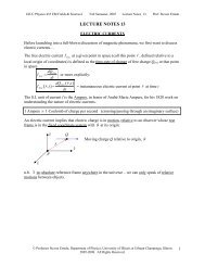
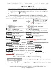
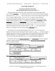
UIUC Physics 435 EM Fields & Sources I Fall Semester, 2007 Lecture Notes 2 Prof. Steven ErredeLECTURE NOTES 2Gauss’ Law / Divergence TheoremConsider an imaginary / fictitious surface enclosing / surrounding e.g. a point charge (or a smallcharged conducting object). For simplicity, use an imaginary sphere of radius R centered on chargeQ at origin:ẑnr ˆ,= Rrˆ E( r) = E( Rrˆ)Infinitesimal Area Element, dAQ θ RϕŷˆxSImaginary/Fictitious Surface, Saka Gaussian Surface of radius Rcentered on charge Q.Area element dA is a VECTOR quantity: dA = dAnˆ = dArˆ. By convention, ˆn is outward-pointingunit normal vector at area element dA. In this particular case (because of spherical symmetry ofproblem): nˆ= rˆΦ ≡∫ E r dAiFLUX OF ELECTRIC FIELD LINES (through surface S): ( )ΦE= “measure” of “number of E-field “lines” passing through surface S, (SI Units: Volt-meters).TOTAL ELECTRIC FLUX ( Φcharge enclosed by surface S.TOTEES) associated with any closed surface S, is a measure of the (total)n.b. charge outside of surface S will contribute nothing to total electric fluxpass through one portion of the surface S and out another – no net flux!)ΦE(since E-field linesConsider our point charge Q at origin. Calculate the flux of E passing through a sphere of radius r:(see above picture) Q 1ΦE= ∫E( r) i dA=rS24πε∫ ⎛ ⎞2rˆi( ⎜ ⎟ r sinθdθdϕrˆ)o S ⎝ r ⎠ = dAinfinitesimal vectorarea element forsphere of radius rdA dAr r d d rˆ2n.b. Vector area element of sphere of radius, r is = ˆ=( sinθ θ ϕ)coordinates.in spherical-polar©Professor Steven Errede, Department of Physics, University of Illinois at Urbana-Champaign, Illinois2005 - 2008. All rights reserved.1

UIUC Physics 435 EM Fields & Sources I Fall Semester, 2007 Lecture Notes 2 Prof. Steven ErredeQΦE=4πε∫θ= o ∫ i =ϕ=o θ= π ϕ=2πThus: sinθdθdϕ( rˆˆr)o2QQ=2 ε = εoo= 12πQ4πε2o∫θ=πθ = osinθdθ QΦE= ∫ E r i dA=sε∴ Gauss’ Law (in Integral Form): ( )enclosedElectric flux through closed surface S = (electric charge enclosed by surface S)/ εooIf ∃ (= there exists) lots of discrete charges q i (ALL enclosed by imaginary / fictitious / Gaussiansurface S), we know from principle of superposition that:N ENETr = ∑ Eir( ) ( )i=1 ( i ) q 1 QΦ = = = = =NNET i enclE ∫ENET r dA ∑S ∫ ESir dA ∑ ∑qii= 1 i= 1 εoεo i=1 εoThen: ( ) i( )If ∃ volume charge density ρ ( r ′), then: Q ( )encl= ∫ ρ r′ dτ′Then using the DIVERGENCE THEOREM: Q 1enclEE( r) dA ( E( r)) dτ ′ Φ = ∫ i = ∇ = = ρ( r)dτS ∫ ivε ε ∫′vThis relation holds for any volume v ⇒ the integrands of ( )v ρ∴ Gauss’ Law (in Differential Form): ( )( r )∇ i E r =oovε∫ dτ ′ must be equal, i.e.:o2©Professor Steven Errede, Department of Physics, University of Illinois at Urbana-Champaign, Illinois2005 - 2008. All rights reserved.

UIUC Physics 435 EM Fields & Sources I Fall Semester, 2007 Lecture Notes 2 Prof. Steven Errede The DIVERGENCE OF E( r) :( )∇ E i r∇ 1 ˆ r E r = r′ dτ′2πε ∫ rCalculate i E( r)directly from ( ) ρ ( )Remember that r is NOT a constant! r ≡r −r′4o vallspacefield sourcepoint pointP S⎡⎤ ⎢1 ˆ⎥⎛ r ⎞ 1 ⎛ ˆ r ⎞ ∇ iE( r) =∇ i⎢⎜ ρ2 ⎟ ( r′ ) dτ′ ⎥ = ∇ ⎜ ρ2 ⎟ ( r′ ) dτ′⎢4πε∫o4πεv ⎝ ⎠ ⎥∫ iro v ⎝ r ⎠⎢ all⎥all⎣ space⎦space ⎛ rˆ⎞ i ⎜ 2 ⎟(see equation 1.100, Griffiths p. 50)⎝r⎠ 3Now: ∇ = 4πδ( r )3−DDiracδ − fcn. ˆ⎛ ⎛ r ⎞ r − r′⎞ i⎜ 2 ⎟ i3⎝ r ⎠ ⎜ r − r′⎟⎝ ⎠3 3Thus: ∇ = 4πδ( r ) or: ∇ ⎜ ⎟ = 4πδ( r − r′) 13 ρ r∴ ∇ iE( r)= 4πδ ( r − r′ ) ρ( r′ ) dτ′=4πε∫εovallspaceGauss’ Law in Integral Form:ρ ( r ) i E( r), thus: i ( ) ∇ =εo( )∫ ( ) ∫ ⎜ ⎟ ∫on.b. now extended over all space!Gauss’ Law in Differential Form: ρ ( r )∇ i E( r)=ε⎛ρ( r′) ⎞ 1 1∇ E r′ dτ′ = dτ′ = ρ( r′ ) dτ′= Q⎝ εo ⎠ εo εoV v vNow apply/use the Divergence Theorem on the volume integral associated with E( r′ ) 1 1∇ E r′ dτ′ = E r dA= ρ r′ dτ′= Qenclεoεo Q ∫ E r′ i dA′=Gauss’ Law in Integral FormSε ( i ( )) ( ) i ( )∫ ∫ ∫v S vThus we obtain: ( )enclooencl∇ i :©Professor Steven Errede, Department of Physics, University of Illinois at Urbana-Champaign, Illinois2005 - 2008. All rights reserved.3

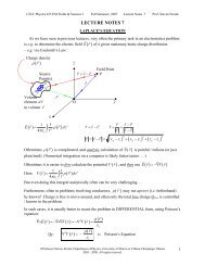
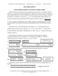
UIUC Physics 435 EM Fields & Sources I Fall Semester, 2007 Lecture Notes 2 Prof. Steven ErredeAPPLICATIONS OF GAUSS’ LAW - very explicit, detailed derivation - Griffiths Example 2.2: Find / determine the electric field intensity E( r)outside a uniformly chargedsolid sphere of radius R and total charge q:Rẑrn ˆ,ˆdraw concentric Gaussiansurface with radius r > Rcentered on solid chargedsphere of radius R.rField Point P @ r Ο ŷ on Gaussian surfaceInfinitesimal area elementdA = dAnˆ= dArˆ2dA = r d cosθdϕ= r2 sinθdθdϕCharged solid ( )Sphere ofRadius R,Total charge q ∫Gauss’ Law: ( ) E r( ) = E( r)ˆrSˆx 1 1 qE r i dA= Qencl= q=ε ε εo o odA = dAnˆ= dArˆ(for Gaussian sphere) ∴ E r dA= E r r dAr = E r dA r r = E r dA( ) i ( ( ) ˆ) i( ˆ) ( ) ( ˆiˆ) ( )= 1Fictitious / Imaginary sphericalGaussian surface S of radius rn.b. by symmetry of sphere:Esphere( r > R) = E( r)ˆri.e. E must be radial!! = ⇐NOTE: E( r) E( r)n.b. Here again, by symmetry,the magnitude of E is constant ∀ (for all)/for any fixed r!!!(on the Gaussian spherical surface). ∴q∫E( r) idA= E( r)dA=S ∫S εo 2= E r dA= E r 4πr =( ) ∫ ( )( )Sqεo q 1 q q 1 q∴ E( r) = 2 = or: E( r) = rˆ=rˆ22 24πεor4πεor4πεor4πεor= Electric field outside a charged sphere of radius R at radial distance r > R from center of sphere.n.b. the electric field (for r > R) for charged sphere is equivalent / identical to that of a point charge qlocated at the origin!!!4©Professor Steven Errede, Department of Physics, University of Illinois at Urbana-Champaign, Illinois2005 - 2008. All rights reserved.

UIUC Physics 435 EM Fields & Sources I Fall Semester, 2007 Lecture Notes 2 Prof. Steven ErredeGAUSS’ LAW AND SYMMETRYUse of (Geometrical / Reflection) symmetry (and any / all kinds of symmetry arguments in general)can be extremely powerful in terms of simplifying seemingly complicated problems!!⇒ Learn skill of recognizing symmetries and applying symmetry arguments to solve problems!Examples of use of Geometrical Symmetries and Gauss’ Lawa) Charged sphere – use concentric Gaussian sphere and spherical coordinatesb) Charged cylinder – use coaxial Gaussian cylinder and cylindrical coordinatesc) Charged box / Charged plane – use appropriately co-located Gaussian “pillbox” (rectangularbox) and rectangular coordinatesd) Charged ellipse – use concentric Gaussian ellipse and elliptical coordinatese) Charged planar equilateral triangle Think aboutf) Charged pyramid these!!APPLICATIONS OF GAUSS’ LAW (CONTINUED)- very explicit detailed derivationGriffiths Example 2.3 Consider a long cylinder (e.g. plastic rod) of length L and radius S that carriesa volume charge density ρ that is proportional to the distance from the axis s of the cylinder / rod –i.e.⎛coulombs⎞ρ(s) = ks⎜ ( meter ) 3 ⎟⎝ ⎠⎛coulombs⎞k = proportionality constant⎜ ( meter ) 4 ⎟⎝ ⎠ a) Determine the electric field E( r)inside this long cylinder / charged plastic rod- Use a coaxial Gaussian cylinder of length l and radius s: (with l

UIUC Physics 435 EM Fields & Sources I Fall Semester, 2007 Lecture Notes 2 Prof. Steven Errede2π s l E( r)=22πks 3l3εoor: ( )inside2 ksE ˆinr = r n.b. ( r≡ s ) ← as used in Griffith’s3εo= < book, page 73( s r S) b) Find ELECTRIC FIELD E( r)outside of this long cylinder / charged plastic rodAgain, use Coaxial Gaussian cylinder of length l ( S): ∫Gauss’ Law: ( )enclS QE r i dA=εEnclosed charge (for s > S):Long charge cylinder ofradius S and length LoQencl233= π klScoaxial Gaussian cylindernˆcyl.= rˆradius s > S and length l

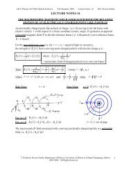
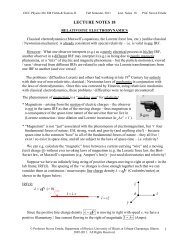
UIUC Physics 435 EM Fields & Sources I Fall Semester, 2007 Lecture Notes 2 Prof. Steven ErredeThen: = 0 = 0 ⎛ ⎞ ⎛ ⎞ ∫ E( r) idA= ( E( r)rˆ) ( dA ˆ) ( ( ) ˆ) ˆ ( ( ) ˆ)ˆS ∫ icylr + ∫ E r r i⎜− dALHS z⎟+∫ E r r i⎜dARHSz⎟⎝ endcap ⎠ ⎝ endcap ⎠cylindrical LHS RHSGaussian Gaussian endcapsurfaceendcap= E r sdld = slE rz= l ϕ=2π( ) ϕ 2π( )∫∫z= 0 ϕ = 0∴ Electric field outside charged rod (s = r > S) : E ( r)out332πklSkS= r=32 i π slεsεo3 oELECTRIC FIELD (INSIDE/OUTSIDE)vs. radial distance sLONG CHARGED CYLINDER(radius S, ρ(s) = ks)Inside (s < S):2 ksE ( ) ˆinr = s3ε Make a plot of E ( r )o E( r)vs. radial distance s:Outside (s > S):3 kS ⎛1 ⎞Eout( r)= ⎜ ⎟sˆ3ε⎝s⎠o( sˆ=rˆ)max( = )E s S2kS=ε3 oVaries as s 2Varies as ~1/s0 s = SRadialDistances8©Professor Steven Errede, Department of Physics, University of Illinois at Urbana-Champaign, Illinois2005 - 2008. All rights reserved.

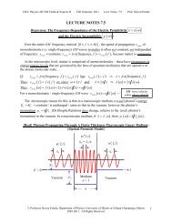
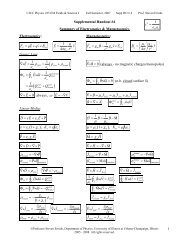
UIUC Physics 435 EM Fields & Sources I Fall Semester, 2007 Lecture Notes 2 Prof. Steven ErredeAPPLICATIONS OF GAUSS’ LAW - very explicit / detailed derivation –Griffiths Example 2.4: An infinite plane carries uniform charge σ (coulombs / meter 2 ).Find the electric field a distance z = z o above (or below) the plane.Use Gaussian Pillboxcentered on ∞ -plane:ẑ“Square”GaussianPillboxΟlhŷlˆxEdge-on Perspective:ẑy = −l/2z = +h/2ˆx (out of page)hz = −h/2ly = +l/2ŷAgain, from the symmetry associated with ∞ -plane, E r = E r zˆ= E z zˆ(above plane), =− (below plane)( ) ( ) ( )E( z) zˆThe Gaussian Pillbox has 6 sides – and thus has six outward unit normal vectors: :nˆˆ5,+ zA 2 (back) nˆˆ2,− xA 5 (top)nˆ,4yˆ−3nˆ, + yˆA 4 (RH side)A 3 (LH side)A 1 (front) nˆ, 1xˆ+ 6nˆ, − zˆA 6 (bottom)©Professor Steven Errede, Department of Physics, University of Illinois at Urbana-Champaign, Illinois2005 - 2008. All rights reserved.9

UIUC Physics 435 EM Fields & Sources I Fall Semester, 2007 Lecture Notes 2 Prof. Steven ErredeThen: E( r) idA= E( r) idA + E( r) idA + E( r)idA+ E r idA + E r idA + E r idA∫ ∫ ∫ ∫S A1 2 31 A2 A3dAdAdA( ) ( ) ( )∫ ∫ ∫4 5 6A4 A5 A6ˆ1=+ dydz xˆ3=+ dxdz yˆ5=+ dxdy zdA2 = dydz ( − xˆ)=− dydz xˆdA4 = dxdz ( − yˆ)=− dxdz yˆdA6 = dxdy ( − zˆ)=− dxdy zˆ E r =+ E z z E r = E z − zˆ=−E z zˆfor z > 0: ( ) ( )ˆfor z < 0: ( ) ( )( ) ( )Again, by symmetry (of plane)n.b. E(z) = constant (at least forfixed z).E r=± E z zNow because ( ) ( )ˆtwo separate regions:z > 0for respectively, we must break up integrals over z intoz < 0z=+ h/2 z= 0 z=+h/2∫ ∫ ∫dz = dz + dzz=− h/2 z=− h/2 z=0Then: y=+ l /2 z=+ h /2 y=+ lˆ/2 z=+hE r dA = E r dydz x + /2 i i E r i − dydz xˆ( ) ( ) ( ) ( ) ( ) ∫ ∫ ∫ ∫ ∫S y=− l/2 z=− h/2 y=− l/2 z=−h/2S y=−l/2x=+ l /2 z=+ h /2 x=+ l /2 z=+h /2 + ∫ E r dxdz y E r dxdz yx=− l/2 ∫ +z=− h/2 ∫ −x=− l/2 ∫z=−h/2x=+ l/2 y=+ l/2 x=+ l/2 y=+l/2 + E r i dxdy zˆ+ E r i − dxdy zˆ( ) i( ˆ) ( ) i ( ˆ)( ) ( ) ( ) ( )∫ ∫ ∫ ∫x=− l/2 y=− l/2 x=− l/2 y=−l/2 y=+l/2z= 0 z=+h/2E( r) • dA= ⎡∫−E( z)zˆixˆdydz + ( + E z zˆix) dydz⎤⎢⎣z=− h/2 z=0⎥⎦y=+l/2z= 0 z=+h/2+ ⎡∫( −E( z)zˆi−xˆ) dydz + ( + E ( z) zˆi−xˆ) dydz⎤y=−l/2⎢⎣z=− h/2 z=0⎥⎦x=+l/2z= 0 z=+h/2+ ⎡∫( −E( z)zˆiyˆ) dxdz + ( + E ( z) zˆiyˆ) dxdz⎤x=−l/2⎢⎣z=− h/2 z=0⎥⎦x=+l/2z= 0 z=+h/2+ ⎡∫( −E( z)zˆi−yˆ) dxdz + ( + E ( z) zˆi−yˆ) dxdz⎤x=−l/2⎢⎣z=− h/2 z=0⎥⎦ ∫( ) ( ) ˆ∫ ∫ ← side A 1 (front)∫ ∫ ← side A 2 (back)∫ ∫ ← side A 3 (RHS)∫ ∫ ← side A 4 (LHS)( ( ) ) ( )x=+ l /2 y=+ l /2 x=+ l /2 y=+l /2∫ ∫ ∫ ∫x=− l/2 y=− l/2 x=− l/2 y=−l/2( )+ −E z zˆi− zˆ dxdy+E z zˆizˆdxdyside A 6 (bottom)side A 5 (top)Now: ( zx ˆi ˆ)= 0 ( zy ˆi ˆ ) = 0 ( xz ˆi ˆ)= 0 ( )And: ( xx ˆi ˆ)= 1 ( yy ˆi ˆ)= 1 ( zz ˆˆ i ) = 1yz ˆi ˆ = 0 etc.10©Professor Steven Errede, Department of Physics, University of Illinois at Urbana-Champaign, Illinois2005 - 2008. All rights reserved.

UIUC Physics 435 EM Fields & Sources I Fall Semester, 2007 Lecture Notes 2 Prof. Steven Errede∴ Because xˆ ⊥ yˆ ⊥ zˆ, no contributions to(i.e. A 1 , A 2 , A 3 and A 4 )∫ E dA i (here) from 4 sides of Gaussian PillboxS⇒ Only remaining / non-zero contributions are from bottom and top surfaces of Gaussian Pillboxbecause nˆˆ5=− z and nˆˆ6=+ z which are (or anti-parallel) to E ( z) z ˆThus, we only have (here): x=+ l/2 y=+l/2 ∫ E ( r) i dA= ( −E( z) zˆ( − zˆ)) dxdyS ∫x l ∫i← side A 6 (bottom)y l=− /2 =− /2x=+ l/2 y=+l/2x=− l/2 y=−l/2( ( ) ˆˆ)∫ ∫ i ← side A 5 (top)+ + E z z z dxdyThese integrals are not over z, and E(z) = constant for z = fixed = z o∴ can pull E(z) outside integral, zz= ˆˆ i 1 − zz ˆˆ i =−1etc. x=+ l/2 y=+l/2∴ ∫ E ( r ) i dA = + E ( z)∫ ∫ dxdy ← side A 6 (bottom)S x=− l/2 y=−l/2x=+ l/2 y=+l/2( )dxdyx=− l/2 y=−l/2( ) ( ) 2 ( )E z+ ∫ ∫ ← side A 5 (top)= E z l + E z l = E z l2 2 22But: l = l× l ≡Α= surface area of top and bottom surfaces of Gaussian Pillbox QenclNow: ∫ E( r) i dA=What is Q encl (by Gaussian Pillbox)?Sεo⎛Coulombs⎞2 2Qencl= σ ⎜2 ⎟×Α ( meters ) = σl ( Coulombs)⎝ meter ⎠ Qencl∴ ∫ E( r) i dA= ⇒ 2E( z) l2 21= σ l εoor: E( z)Sε= ⎛ ⎞ σ σ⎜ ⎟⎝2⎠= εo 2εoozˆ, for z 0Vectorially: E( z) σ + >=⎛ ⎞⎜ ε ⎟{ − zˆ, for z

UIUC Physics 435 EM Fields & Sources I Fall Semester, 2007 Lecture Notes 2 Prof. Steven Errede E( r)from ∞ - plane (slight return):Note that in the initial process of setting up the Gaussian Pillbox, if we’d shrunk the height h of thePillbox to be infinitesimally small, i.e. h → δh and then took the limit δh→0, the contributions to∫ E S( r ) dA i from (infinitesimally small) sides of (A 1 , A 2 , A 3 and A 4 ) Gaussian Pillbox would(formally) have vanished (i.e. = 0) independently of whether integrand ( E ( r)dA i ) vanished on thesesides (or not). Only top and bottom surfaces contribute to ∫ E S( r ) dA i then (here).So using this “trick” of the shrinking Pillbox at a surface / boundary very often can be useful, tosimplify doing the problem.This explicitly shows that (sometimes) there is more than one way to correctly do / solve a problem– equivalent methods may exist.→ It is very important, conceptually-speaking to have a (very) clear / good understanding of how todo these Gauss’ Law-type problems the “long’ way and the “short” way!12©Professor Steven Errede, Department of Physics, University of Illinois at Urbana-Champaign, Illinois2005 - 2008. All rights reserved.

UIUC Physics 435 EM Fields & Sources I Fall Semester, 2007 Lecture Notes 2 Prof. Steven Errede The Curl of E( r) : ( ∇×E( r)) 1 ⎛ q ⎞= ⎜ ⎟rˆ4πεo ⎝r⎠(note: r ≡r − r ′ = rhere because r′ = 0 - charge q located at origin!!!) is radial (i.e. in ˆr − direction) due to spherical symmetry of problem (rotationalFirst, study / consider simplest possible situation: point charge at origin: E( r) 2Thus (here), E( r)invariance), thus static E -field has no rotation/swirl/whirl ⇒ no curl! (Read Griffith’s Ch. 1 on curl) ⇒∇× E r = (must = 0)( ) 0Let’s calculate:bLine integral ∫ E a( ) i as shown in figure below:ẑ ˆrˆxẑˆϕbr b θ θ ŷq ŷ Οr a d ϕ ˆϕad ˆxIn spherical coordinates: d = drrˆ+ rdθθ + r sinθdϕϕˆ 1 ⎛ q ⎞E( r) i d = rˆ drrˆ+ rd ⎜+ rsin2 ⎟ iπε ⎝r⎠4o{ θθ θϕϕˆ}Again: rr= ˆˆ i 1 rˆ i θ = 0 rˆ i ˆ ϕ = 0 ˆr , θ , and ˆϕ are mutuallyθθ= i 1 θ i rˆ= 0 θϕ= i ˆ 0 orthogonal basis vectorsˆ ϕi ˆ ϕ = 1 ˆ ϕ i rˆ = 0 ϕθ= ˆi 0 (form ortho-normal basis) 1 ⎛ q ⎞∴ E( r) i d = ⎜ dr2 ⎟πε ⎝r⎠∫b4ob 1 b q −1 ⎛q⎞1 ⎛ q q ⎞ q ⎛ 1 1 ⎞E r i d = dr4πε ∫ =a⎜ ⎟ = ⎜ − ⎟= ⎜ − ⎟or 4πε o ⎝ r ⎠ 4πε o ⎝ra rb ⎠ 4πεo ⎝ra rb⎠Thus: ( )2ar a = distance from origin Ο to point a. r b = distance from origin Ο to point b.The line integral ( )∫ E r di around a closed contour C is zero!rra©Professor Steven Errede, Department of Physics, University of Illinois at Urbana-Champaign, Illinois2005 - 2008. All rights reserved.13

UIUC Physics 435 EM Fields & Sources I Fall Semester, 2007 Lecture Notes 2 Prof. Steven Errede∫ E r d i = This is not a trivial result! (Not true ∀ vectors!!)C(But is true for static E -fields)i.e. ( ) 0Use Stokes’ Theorem (See Griffiths, Ch. 1.3.5, p. 34 and Appendix A-5)∫S ( ∇× E( r)) idA= E( r) id=0 ∫arbitrary closed arbitrary closedsurface S contour C (on S)∫ ( ∇× ) dA=0SSince E( r)C i must be / is true for arbitrary closed surface S, ∇× E r =this can only be true for all ∀ closed surfaces S IFF (if and only if): ( ) 0Can use the Principle of Superposition to show that:N E r E r∑i( ) = ( ) =2TOT i ii= 1 4πεo i=1 ri1N∑qrˆ = E1 r + E2 r + E3 r + ... + ENr( ) ( ) ( ) ( )← i = 1,2,3. . . N discrete charges, and r = ( r −r)ẑ r2r3i E( r)@ field point Psource points q 2 q 3 P@ r 1, r 2… r Nr1q 1 r r 2 3r r 1Ο ŷi N ∑N∑( ) Then: ∇× E ( r) =∇× E ( r) = ∇× E ( r)TOT i ii= 1 i=1ˆx ri = ri= r −riN⎛ 1 ⎛ q ⎞ ⎞i= ∑∇× ˆ⎜ ⎜ 02 ⎟r=ii=1 4πε⎟⇐ n.b. all individual terms = 0 !!!⎝ o ⎝ ri⎠ ⎠ N 1 ⎛ 1 ⎞∇× E ˆTOTr = ∑ qi ∇× ⎜ ⎟ ri= 04πε o i=1 ⎝ ri⎠or: ( )2It can be shown that ∇× E( r) = 0 FOR ANY STATIC CHARGE DISTRIBUTIONSTATIC = NO TIME DEPENDENCE / VARIATION14©Professor Steven Errede, Department of Physics, University of Illinois at Urbana-Champaign, Illinois2005 - 2008. All rights reserved.

UIUC Physics 435 EM Fields & Sources I Fall Semester, 2007 Lecture Notes 2 Prof. Steven Errede ∇× E r =( ) 0 HOLDS FOR:• Static Discrete/Point Charges q( r )• Static Line Charges λ ( r )• Static Surface Charges σ ( r )• Static Volume Charges ρ ( r )Again, this not trivial (we’ll see why, soon. . . )All Static Charge DistributionsOne other (very important) point about the mathematical & geometrical nature of vector fields: The nature of a (physically-realizable) vector field Ar ( ) is fully specified if both its divergence∇ Ar ∇× Ar are known.i ( ) and its curl ( )This is a consequence of the so-called Helmholtz theorem – see/read Appendix B of Griffiths book.The Helmholtz theorem also has an important corollary: Any differentiable vector function Ar ( ) that goes to zero faster than 1 r as r →∞can be expressedas the gradient of a scalar plus the curl of a vector: ⎛ 1 ∇′ iAr( ′) ⎞ ⎛ 1 ∇ ′ × Ar ( ′)⎞Ar ( ) =∇ − dτ′ +∇×dτ′⎜ 4π∫v′ ⎟ ⎜4π∫v′⎟⎝ r ⎠ ⎝ r ⎠ For the case of electrostatics: ∇ i E( r) = ρ ( r) εo and ∇× E( r) = 0 Thus: ⎛ 1 ∇′ iE r′ 1E( r)=∇ − dτ ′+∇× ⎜⎜ 4π∫v′⎟⎝r ⎠⎜4π∫v′r⎝1 ⎛ ρ ( r′) ⎞ =− ∇ ⎜ dτ′ ⎟ =−∇ V ( r)4πε∫v′o ⎝ r ⎠( ) ⎞ ⎛ ∇× ′ E( r′)⎞dτ′ ⎟⎟⎠i.e. E( r) =−∇V ( r)with V ( r)≡1 ρπε ∫ ′r4vo( r′)dτ′= Electrostatic PotentialSI Units:VoltsThis result is valid e.g. in electrostatics for localized (i.e. finite spatial extent) charge distributions.For infinite-expanse charge distributions (n.b. these are unphysical/artificial!), we must appeal to(more sophisticated) mathematical formalisms than the Helmholtz theorem…©Professor Steven Errede, Department of Physics, University of Illinois at Urbana-Champaign, Illinois2005 - 2008. All rights reserved.15