Lecture Notes 07.5 - University of Illinois High Energy Physics

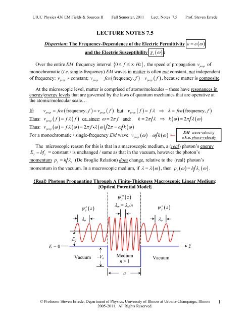
UIUC Physics 436 EM Fields & Sources II Fall Semester, 2011 Lect. Notes 7.5 Prof. Steven ErredeLECTURE NOTES 7.5Dispersion: The Frequency-Dependence of the Electric Permittivity ε = ε( ω)and the Electric Susceptibility χe( ω ) :0 ≤ ≤∞ , the speed of propagation vpropofmonochromatic (i.e. single-frequency) EM waves in matter is often not constant, not independentof frequency: vprop≠ constant; vprop= fcn( frequency, f ) = vprop( f ) , because matter is composite.Over the entire EM frequency interval { f Hz}At the microscopic level, matter is comprised of atoms/molecules – these have resonances inenergy/energy levels that are governed by the laws of quantum mechanics that are operative atthe atomic/molecular scale…If: vprop= fcn( frequency, f ) = vprop( f ) but: vprop( f ) = fλ ⇒ λ = fcn( frequency, f )Thus: vprop( f ) = fλ( f ) or, since: ω ≡ 2πf and: k ≡ 2π λ ⇒ k ( ω) ≡ 2π λ( ω)Thus: vprop( ω) = fλ( ω) = 2π fiλ( ω) 2π = ω k( ω)For a monochromatic / single-frequency EM wave v ( ω) = ω k( ω)←The microscopic reason for this is that in a macroscopic medium, a (real) photon’s energyEγ= hfγ= constant / is unchanged / same as that in the vacuum, however the photon’smomentum pγ= h λγ(De Broglie Relation) does change, relative to the {real} photon’sλ λ ω p ω = h λ ω .momentum in the vacuum. In a macroscopic medium, if = ( ) , then ( ) ( ){Real} Photons Propagating Through A Finite-Thickness Macroscopic Linear Medium:{Optical Potential Model}λ m = λ o /npropooψ ( z)ψγ ( z)γψmγ( z)γEM wave velocitya.k.a. phase-velocityγλ oλ oE = 0E γẑVacuum−V oMediumn > 1Vacuuma© Professor Steven Errede, Department of Physics, University of Illinois at Urbana-Champaign, Illinois2005-2011. All Rights Reserved.1

UIUC Physics 436 EM Fields & Sources II Fall Semester, 2011 Lect. Notes 7.5 Prof. Steven ErredeMacroscopically, the frequency-dependence of the wavelength λ λ( ω)( ) = 2π λ( ω), and linear momentum ( )= , or wavenumberk ωp ω associated with macroscopic EM wavespropagating in a macroscopic, linear/homogeneous/isotropic medium arises from the frequencydependenceof the macroscopic electric permittivity ε ( ω ) (or equivalently the electricsusceptibility χe( ω ) since:ε ω = ε 1+ χ ω .( ) o( e( ))The frequency dependence of the macroscopic electric permittivity ε ( ω ) is known as dispersion;a medium that has ε ≠ constant with varying frequency is known as a dispersive medium.For non-magnetic/non-conducting linear/homogeneous/isotropic media, the index of refraction= . Thus if ε = ε( ω) = εo( 1+ χe( ω)) then n( ω) ε( ω) εon ε ε o= .For a wave packet (= a group {= superposition/linear combination} of waves of many frequencies– as explained by Mssr. Fourier), the envelope of the wave packet travels with (in general,frequency-dependent) group velocity:vgroup( ω)( ω)" "dω1 ⎡dk⎤≡ = = ⎢ ⎥dk ( ω) dk ( ω)dω ⎣ dω⎦A propagating wave packet: vp( ω) = vphase( ω) = ω k( ω)( ) ( ) ( )−1vgω = vgroupω ≡⎡dk ω dω⎤−⎣ ⎦1If the phase velocity vp( ω) ω k( ω)−1( ω) = ⎡ ( ω) ω⎤≠ ( ω)v dk d vgroup= is frequency dependent, and⎣ ⎦ phase{e.g. as in the case for surface waves on water, wherevp= 2vg} the exact relationship between vphaseand vgroupdepends on the detailed nature of themedium (as we shall soon see. . . ).Note that energy carried by a wave packet travels at the group velocity, vgroupand not at thephase velocity vphase. Note that in certain circumstances, vphasecan exceed c {= speed of light inthe vacuum} but in these situations, no energy (and/or information) is transmitted – these aretransmitted at vgroup< c always, by causality… A physical/mechanical example: calculate thephase velocity of the intersection point of the two halves of a scissors as the blades of thescissors are closed. {Ans:vscissorsp→∞!!!}2© Professor Steven Errede, Department of Physics, University of Illinois at Urbana-Champaign, Illinois2005-2011. All Rights Reserved.

UIUC Physics 436 EM Fields & Sources II Fall Semester, 2011 Lect. Notes 7.5 Prof. Steven ErredeAn Important Detail:Physically, the phase velocity vphase( ω) ≡ ω k( ω)= a single point on the ω vs. ( )whereas the group velocity v ( ω) ≡ " dω dk( ω)"= the slope of the ω vs. ( )groupk ω curve,k ω curve:← Technically, making this plot is wrong !!!Why is this plot technically wrong ???Because ω is the independent variable {always plotted on the axis of abscissas (i.e. the x-axis)}and k ( ω)is the dependent variable {always plotted on the axis of ordinates (i.e. the y-axis)}Thus, the technically correct way is to plot k ( ω ) vs. ω : {i.e. k depends on ω , not vice-versa!}Then: v ( ω)group( ω) ⎞ ⎡dk( ω)⎛dk⎤≡ 1 ⎜ ⎟=⎢ ⎥⎝ dω⎠ ⎣ dω⎦−1i.e. vgroup( ω) ≡ { k( ω)vs ω}1 slope of . graph :© Professor Steven Errede, Department of Physics, University of Illinois at Urbana-Champaign, Illinois2005-2011. All Rights Reserved.3

UIUC Physics 436 EM Fields & Sources II Fall Semester, 2011 Lect. Notes 7.5 Prof. Steven ErredeDispersion Phenomena in Linear DielectricsIn a non-conducting, linear, homogeneous, isotropic medium there are no free electrons(i.e. ρfree ( r ) = 0 ). Atomic electrons are permanently bound to nuclei of atoms comprising themedium. ⇒∃ no preferential direction / no preferential directions in such an {isotropic} medium.Suppose each atomic electron (charge –e) in a dielectric is displaced by a small distance r E r .from its equilibrium position, e.g. by application of a static electric field ( )The resulting macroscopic electric polarization (aka electric dipole moment per unit volume) is: 3Ρ ( r) = nep( r)where: n e = (atomic) electron number density (#e m ) p r = −er{here}, where r is theand the {induced} atomic/molecular electric dipole moment is: ( ){vector} displacement of the atomic electron from its equilibrium { E = 0} position. Ρ r = n p r =−n erThus: ( ) ( )eeThe atomic electrons are each elastically bound to their equilibrium positions with a force constant ke. The force equation for each atomic electron is thus: Fe( r) =− eE( r)= kerThe static polarization is therefore given by: ( ) ( ) ( )2 ⎛−eE r ⎞ neeΡ r = nep r =− neer =− nee =+ E r⎜ k ⎟eke⎝ ⎠However, if the E ikz ( −ωt)-field varies with time, i.e. E = E( r,t)= E oee.g. due to amonochromatic EM plane wave incident on an atom, the above relation is incorrect !A more correct {“semi-classical”} way to treat this situation is to consider the bound atomicelectrons as classical, damped, forced harmonic oscillators, as mathematically described by thefollowing differential equation:mr e+ meγr + kr e=−eE ( r ) ← inhomogeneous 2 nd -order differential equation2∂ r () t ∂r()t me + m2 eγ+ ker n.b. we have neglected the() t =−eE( r,t)← ∂t ∂t ev × B eE term here...ma e( )( )Velocity-dependentdamping termγ ≡ damping constantPotential Force(binding of atomicelectrons to atom)meDriving Force= electron mass = 9.1×10−31kgSuppose the driving / forcing term varies sinusoidally/is harmonic/periodic in time with iωtF r, t =− eE r,t =−eE e −i tr because E ω( r,t) = E e − rˆ.angular frequency ω , i.e. ( ) ( ) ˆn.b. The electric field E is now complex E .eoo4© Professor Steven Errede, Department of Physics, University of Illinois at Urbana-Champaign, Illinois2005-2011. All Rights Reserved.

UIUC Physics 436 EM Fields & Sources II Fall Semester, 2011 Lect. Notes 7.5 Prof. Steven ErredeThen the inhomogeneous force equation becomes:In the steady state, we have:i tmr − ω+ mγr + kr =−eEe rˆ with ( ) ( ) ˆe e e oi tmr − ω+ mγr + kr =−eEe rˆe e e or t = r t r .Since r physically represents the {vector} spatial displacement of each atomic electron from itsequilibrium { E = 0i ω r t = r ω e − t r r t is now complex}.} position, then: ( ) ( ) ˆ {n.b. ( )oThus:i tmr − ω+ mγr + kr =−eEe rˆe e e o2∂ r ( t) ∂r( t) me + m ,2 eγ+ ker t =−eE r t∂t∂t−mωre ωe2 −i toeo() ( )−i t− iωmγre ωi t+ kre − ω2( ω ω γ)e om − k + i m r= eE e e e o oi t=−eE e − ωoDivide this equation through by m :Define:2⎛ k ⎞eω0≡ ⎜ ⎟⎝me⎠2 2Then: ( ω ω γω)e⎛2⎛ k ⎞ ⎞eeω − ⎜ ⎟+ iωγro= E⎜ m ⎟⎝ ⎝ e ⎠ ⎠ mekeor: ω0≡ = characteristic/natural resonance {angular} frequency.m⎛ e ⎞− + i r =⎜ ⎟E⎝ ⎠0 o omee⎛ e ⎞⎜ Em ⎟o =⎝ ⎠=⎡⎣ω − ω0+ iγω⎤⎦e or: ro( ω) 2 2 {n.b. Ρ is now complex and frequency-dependent!!!}iωtNow: Ρ ( rt , ) =− ner( t) =−ner( ω) e − rˆe e ooAtomic electron spatialdisplacement amplitude{n.b. complex!}Thus: ( rt)2e iωt( )( ˆo )e2−n⎛e⎞ee −neE e rm⎜ m ⎟Ρ ,⎝ ⎠ = =+Ert ,2 2 2 2⎣⎡ω − ω0 + iγω⎦ ⎤⎣⎡ω0−ω −iγω⎦⎤( )⇐n.b. Note the re-ordering ofterms in the denominatorω = : ( ω 0)For 0⎛2 2e ⎞en⎛e⎞⎜ e2m ⎟ ⎜em ⎟⎝ ⎠ ⎝ e⎠⎛ne⎞e2 o o oωk0⎛ e ⎞ ke⎜⎝ ⎠m ⎟enΡ = = Er ˆ= Er ˆ=⎜ ⎟Er ˆ ⇐Note also that the phase of {complex} ( ω) lags behind E ( ω)by a phase angle of:Ρ ⎝⎠Static polarization Ρ ( ω = 0)depends on the {angular} frequency ω – i.e. Ρ ( ω) is in-phase with E φΡ( ω)⎡Im( Ρ( r,t)1) ⎤ ⎡1 γω ⎤−−= tan ⎢ ⎥ = tan ⎢ ⎥ ⇐2 2⎢Re( Ρ( r,t)) ⎥ ⎢⎣( ω0−ω⎣⎦) ⎥⎦n.b. The damping constant γhas the same units as ω :radians/sec© Professor Steven Errede, Department of Physics, University of Illinois at Urbana-Champaign, Illinois2005-2011. All Rights Reserved.5

UIUC Physics 436 EM Fields & Sources II Fall Semester, 2011 Lect. Notes 7.5 Prof. Steven ErredekeWhen: ω < ω0= , φ Ρ> 0 ⇒ Ρ klags E . When:eω > ω0= , φ Ρ< 0 ⇒Ρ leads E .memeFrom the above formula, note that if the damping constant, γ = 0 then φ Ρ= 0 , the electricΡ ωbecause if 0 ImΡ r, t = 0,polarization ( )is then always in-phase with ( ) E ω( )γ = , then ( )i.e. the electric polarization Ρ ( ω)is purely real! Physically, a damping constant of γ = 0 meansthat the width Γ= γ 2πof the atomic/molecular resonance is infinitely narrow, and thus there areno dissipative processes (i.e. energy loss mechanisms) present at the microscopic atomic/molecularlevel in this macroscopic medium! Note also that γ has physical/SI units of radians/second.Note further that E in the above expression is actually E int− the internal macroscopic electric field of the dielectric: E = Eint= Eext+ EP, the sum of the macroscopic external applied electricfield and the macroscopic electric field due to the polarization of the dielectric medium.The electric field due to polarization of the medium is:EP1 = − Ρε2 1 n⎛e⎞ Thus: E = Eint= Eext− Ρ e ⎜ m ⎟e⎡ 1 ⎤Therefore: Ρ ⎝ ⎠ = E2 2ext− Ρ⎢ ⎥ where: ω0≡3εo⎡⎣ω 3o−ω −iγω⎤⎦ ⎣ εo ⎦Now solve for Ρ : Skipping writing out some of the {tedious} complex algebra, we obtain:3 oSee P435 Lect. Notes 10, p. 1-6,see also P435 Lect. Notes 9, p. 26keme2n⎛e⎞⎜ m ⎟eeΡ=⎝ ⎠⎡2 2ω1− ω − iγω⎤⎣E⎦extwhere:22 ⎛ne⎞ωe1≡ ω0 − ⎜ 3εome⎟⎝ ⎠=effective angularresonance frequency ofbound atomic electronsThis formula is essentially identical e.g. to the {complex} displacement amplitude formula fora driven harmonic oscillator, and/or that for the {complex} AC voltage amplitude in an LCRcircuit, and for many other physical systems exhibiting a {damped} resonance-type behavior.Now ifEext= E -field associated with a monochromatic plane EM wave propagating in aikz ( −ωt)Eextz,t = Eoe, then because of the linear relationship between theikz tE −ωz,t = E e xˆ, Gauss’ Law becomes (since ρ ( r ) = 0 ):dielectric medium: ( )polarization Ρ and ( )( )extofor EM plane wave1∇ E iext=− ∇iΡ= ρbound= 0εoρ r = and J = 0 } becomes:The wave equation {for a dielectric medium with ( ) 0free22 2 μon⎛e⎞ e22 1 ∂ Eext∂Ρ ⎜ m ⎟e ∂ Eext∇ Eext− = μ2 2 o=⎝ ⎠2 2 22c ∂t ∂t ⎡ω t1−ω −iγω⎤∂ 1with:2⎣⎦cfreefree= ε μoo6© Professor Steven Errede, Department of Physics, University of Illinois at Urbana-Champaign, Illinois2005-2011. All Rights Reserved.

UIUC Physics 436 EM Fields & Sources II Fall Semester, 2011 Lect. Notes 7.5 Prof. Steven ErredeOr: 1 ⎡ ⎛ ne ⎞ 1 ⎤ ∂ E2 22e ext∇ Eext= ⎢1 2+⎜ ⎟⎥2 22c ⎢ εome⎡ω t1−ω −iγω⎤⎥∂⎣⎝ ⎠⎣ ⎦⎦with:22 neeω1 ≡ ω0−3εmoThe general solution to this dispersive wave equation is of the form:ikz ( −ωt)E z t = E eext( , )owith complex k = k+iκ and⎛ ne22 2e= 12 ⎢ + ⎜ ⎟ 2 2 ⎥ .c εomeω1−ω −iγωkω ⎡⎣⎝⎞⎠1⎤⎦Thus, we also see here that the complex wavenumber k = k+iκ is explicitly dependent onk ω = k ω + iκ ω .the angular frequency ω , i.e. ( ) ( ) ( )We further see that monochromatic plane EM waves propagating in a dispersive dielectric ikz ( −ωt) −κz ikz ( −ωt)E z,t = E e = E e e ,medium are exponentially attenuated, because ( )i.e. the κ( ω) m k( ω)( )ext o o=I term corresponds to absorption/dissipation in the macroscopicdielectric, and is physically related to, and thus proportional to the damping constant γ .and thus the macroscopic{here} is also {now} complex and is also frequency-dependent, i.e.Note that we can also write: Ρ( zt ,, ω) ≡ε oχe( ω) Eext( zt ,, ω)electric susceptibility χe( ω) χ ( ω) ≡ χ ( ω) + iζ ( ω). The ζ ( ω) m χ ( ω)e e ee( e )=I term corresponds to absorption/dissipationin the macroscopic dielectric, and is physically related to, and thus proportional to the dampingconstant γ . The corresponding dissipative energy losses at the microscopic, atomic/molecularlevel in the macroscopic dielectric ultimately wind up as heat!⎛2 2e ⎞ een⎛ ⎞⎜ ⎟ e⎜ ⎟nm⎛ε⎞ mΡ⎝ ⎠ ⎝ ⎠ =2 2 ext=⎜ ⎟ 2 2⎣⎡ω1 −ω −iγω⎦ ⎤ ⎝εo ⎠⎣ ⎡ω1−ω −iγω⎦⎤eoeSince: ( zt , ) E ( zt , ) E ( zt , )ext22 neewith ω1 = ω0−3εmoe2⎛ ne ⎞ 1⎜ ⎟⎝ ⎠⎣ ⎡ ⎤⎦e∴ The complex electric susceptibility is: χ ( ω ) = ≡ χ ( ω ) + i ζ ( ω )e 2 2e eεomeω1− ω − iγωNow before we go much further with this, we need to discuss another aspect of our model– namely that in most linear dielectric materials, the atoms comprising the material are multielectronatoms, and consequently there are many different binding energies – the outer shellatomic electrons are weakly bound, hence have small ke, and thus small ω0= ke me, whereasthe inner-shell electrons are much more tightly bound, hence have larger k e, larger ω0= ke me.Furthermore, in complex media, i.e. dielectrics with more than one kind of atom, electronscan be shared between atoms – i.e. they are bound to molecules e.g. the π-electrons in benzenering / aromatic hydrocarbon-type compounds, which can be weakly bound in some molecules.© Professor Steven Errede, Department of Physics, University of Illinois at Urbana-Champaign, Illinois2005-2011. All Rights Reserved.7

UIUC Physics 436 EM Fields & Sources II Fall Semester, 2011 Lect. Notes 7.5 Prof. Steven ErredeThus, there can be also be {molecular} resonances e.g. in the microwave and infra-redregions of the EM spectrum – atomic resonances are typically in the optical and UV regions{for the outer-most shell electrons}, as well as in the far UV and x-ray regions {for the innershellelectrons}!Allowing for all such resonances, we can write the {complex} electric polarization Ρ as asummation over all of the resonances present in the linear dielectric as follows:neΡ =m2⎛noscf ⎞ ⎡ω −ω −iγ ω⎤⎟⎣⎦⎠ej( zt , ) ⎜⎟E ( zt , )and where:Physically:⎜⎝∑2 2e j=1 1 j joscfjextwhere: ω2nee≡ ω − and: ω0j≡3εm21j0 j≡ oscillator strength of j th resonance, defined such thatoscfj= fractional strength of the j th resonance and γj= 2π*width of the j th resonance.Thus, we see that the complex electric susceptibility χ ( ω) ≡ χ ( ω) + iζ ( ω)e e eoen∑j=1foscj is:2 noscχ ω ⎛ ne ⎞⎛f ⎞e ⎜ ⎟ 2 2e eεome j 1 ω1jω iγ χ ω ζ ω⎜∑⎝ ⎠ = ⎡ − −jω⎤⎟⎝ ⎣ ⎦⎠j( ) =e≡ ( ) + i ( )The complex electric permittivity ε ( ω) = εo( 1+ χe( ω)) ≡ ε( ω) + iς( ω)dielectric medium is:= 1 of a dispersive, linear⎛2 noscε ( ω ) ε χ o e( ω ) ε ⎛ ne ⎞ f ⎞ = + =o+ ⎛ ⎞⎜ ⎟ ≡εome j 1 ω1jω iγ ε ω + ς ω⎜ ⎝ ⎠ ⎜= ⎡ − −jω⎤⎟⎣ ⎦ ⎟⎝ ⎝⎠⎠j( 1 ) ⎜e1 ⎜∑⎟⎟( ) i ( )2 2with the relations: ε ( ω) =R e( ε( ω)) = εo( 1+χe( ω)) and ς ( ω) =I m( ε( ω)) = εoζe( ω)km .Thus, monochromatic plane EM wave solutions to the dispersive wave equation are of the form:ikz ( −ωt)E z,,t ω = E ek ω = k ω + iκ ω ≡ ε ω μ ω( )Thus: ( ,, ω)owith {complex} wavenumber ( ) ( ) ( ) ( ) o ( −ω) −κzE z t = E e = E e eikz t ikz text o oexponentialdampingof EM wave ( −ω) is equivalentIntroducing a {frequency-dependent} complex wavenumber k( ω) = k( ω) + iκ( ω)to introducing a {frequency-dependent} complex index of refraction n( ω) = n( ω) + iη( ω) .For a linear, dispersive dielectric, the complex index of refraction and complex wavenumber are{simply} related to each other by: k ⎛ω⎞( ω) = ⎜ ⎟ n( ω)⎝ c ⎠eje8© Professor Steven Errede, Department of Physics, University of Illinois at Urbana-Champaign, Illinois2005-2011. All Rights Reserved.

UIUC Physics 436 EM Fields & Sources II Fall Semester, 2011 Lect. Notes 7.5 Prof. Steven Errede( k ω + iκ ω ) = ( n( ω) + iη( ω)) = n( ω) + i η( ω)∴ ( ) ( )⎛ω⎞= ⎜ ⎟⎝ c ⎠⇒ k( ω) n( )⎛ω⎞ ⎛ω⎞ ⎛ω⎞⎜ ⎟ ⎜ ⎟ ⎜ ⎟⎝ c ⎠ ⎝ c ⎠ ⎝ c ⎠ω and⎛ω⎞κ( ω) = ⎜ ⎟ η( ω)⎝ c ⎠n ωThe complex index of refraction ( ) is related to the complex electric permittivity ε ( ω) = 1+ χe( ω)and thus the complex electric susceptibility χ ( ω)via the relation n ( ω) = ε( ω) ε = 1+ χ ( ω),( )e2oscn2ε ω⎛ ne ⎞⎛f ⎞ejSquaring both sides: n( ω)= = 1 + χe( ω)= 1 + ⎜ ⎟ 2 2εo εome ⎜∑⎝ ⎠ j=1 ⎡ω1j−ω −iγ jω⎤⎟⎝ ⎣ ⎦ ⎠But:2 2 nosc2 ω ⎛ nef ⎞ej2 2k⎛ ⎞ ⎛ ⎞( ω) = 1 ⎡ ⎤⎜ ⎟ ⎜ + ⎜ ⎟⎢⎥ ⎟ = k( ω) + iκ( ω)= k ω + 2ikω κ ω + κ ω2 2⎝ c ⎠ ⎜ εome ⎢∑⎝ ⎠ j=1 ⎡⎣ω1j − ω − iγ jω⎤⎦ ⎥⎟⎝ ⎣⎦⎠2( ) ( ) ( ) ( ) ( )oe⎛ c ⎞ = ⎜ ⎟ then:⎝ω⎠Since: n( ω) k( ω)⎛ ⎞ f= = +⎜ ⎟⎢ ⎡ ⎤⎥⎝ω⎠ ⎝ε ⎠⎢ ω ω γ ω⎤⎣ ⎣ ⎦ ⎥⎦2 2 nosc2 ⎛ c ⎞ 2 neej( ω) k⎜ ⎟ ( ω)1 ∑ 2 2ome j=1 ⎡1 j− −ijn2 2 2( n( ω) iη( ω)) n ( ω) 2 in( ω) η( ω) η ( ω)= + = + −1 1 x + iy x + iyUsing the “standard” trick: z = = =2 2x −iy x − iy x + iy x + yx+ y , R e( z ) = and I m2 2( z) =2 2Then equating the real and imaginary parts of the LHS & RHS of the above equation, we obtain:xxy+ yn2n( ω) η ( ω)2 2⎡2osc 2 2 ⎤nne( 1 )e ⎢ fjωj−ω⎥− = 1+ 2 22ε j 12 2om⎢∑e = ⎡⎥( ω1j− ω ) + γjω⎤⎢ ⎢⎣⎥⎦⎥⎣⎦( ωηω ) ( )⎡⎤2 noscnee ⎢ fjγωj ⎥=2 22ε j 12 2om⎢∑e = ⎡⎥( ω1j− ω ) + γjω⎤⎢ ⎢⎣⎥⎦⎥⎣⎦2 equations and 2 unknowns:n ω & η ω{ ( ) ( )}→ solve for n( ω) & η( ω )First define: α ( ω)βxx( ω)⎡osc 2 2fj ( ω1j−ω)2( 1 j ) j2 n⎛ nee⎞⎢ ⎥∑ε j 12 2 2 2ome= ⎡ ω ω γ ω ⎤≡ ⎜ ⎟⎢ ⎥⎝ ⎠⎢⎢− +⎣⎥⎦⎥⎣⎦⎡oscfj ( γωj )2( 1 j )2 n⎛ nee⎞⎢ ⎥j 12 2 2 2⎝ε ome⎠ = ⎡ ω − ω + γjω⎤∑ (n.b.x ( ) 0≡ ⎜ ⎟⎢ ⎥⎢ ⎢⎣⎥⎦⎥⎣⎦⎤⎤β ω > , is always positive)Then: n 2 ( ω) − η 2( ω) = + α ( ω)and n( ω) η( ω) = β ( ω)⇒ η ( ω) = β ( ω) 2n( ω)1x2xx© Professor Steven Errede, Department of Physics, University of Illinois at Urbana-Champaign, Illinois2005-2011. All Rights Reserved.9

UIUC Physics 436 EM Fields & Sources II Fall Semester, 2011 Lect. Notes 7.5 Prof. Steven Errede2Thus: n ( )n( ω)( ω)⎛β⎞xω − ⎜= + α ω2n⎟⎝ ⎠( )( ω)2( 1x ( ))24⎛βx⎞2( 1x ( )) n ( )ω − ⎜ ⎟ = + α ω ω⎝ 2 ⎠β ( ) 2xωω − 1+ αxn ω − ⎜⎛ ⎟⎞ = 0⎝ 2 ⎠4 2Or: n ( ) ( ) ( )2Define: x≡ n ( ω). Temporarily we suppress the ( )2Then: x ( α )⎛βx⎞− 1+ xx− ⎜ ⎟ = 0⎝ 2 ⎠2→2⇐ multiply equation through by n ( ω )⇐2ax bx cω -dependence in the following:+ + = 0 with 1Solutions / roots of this quadratic equation are of the general form:⇒2n.b. This may look like a quartic equation,but it is actually a quadratic equation !!!⎛β⎞= − + , c =− ⎜ ⎟⎝ 2 ⎠2− b±b −4acx =2aa = , b ( 1 α )2 ⎛βx⎞+ ( 1+ αx) ± ( 1+ αx)+ 4 ⎜ ⎟⎝ 2 ⎠ 1 2 2x = =⎡( 1 + αx) ± ( 1 + αx)+ β ⎤x2 2⎢⎣⎥⎦2⎡1 ⎛ β ⎞1 1 1x= + ⎢x± +⎜ 2 ⎢ ⎜( 1+αx ) ⎟⎢⎣⎝ ⎠i.e. x ( α )2⎤⎥⎥⎥⎦n.b. the term:⎛ β ⎞x⎜> 0( 1+αx ) ⎟⎝ ⎠2→ Must select +ve root on physical grounds, sincex2≡ n > 0 .⎡2 1 ⎛ β ⎞1 1 1x= = + ⎢ + +⎜ 2 ⎢ ⎜( 1+αx ) ⎟⎢⎣⎝ ⎠∴ x n ( α )Finally, we obtain:2⎤⎥⎥⎥⎦n⎡2 ⎤⎛1+αx( ω) ⎞ ⎛ βx( ω)⎞≡R ( ) = ⎢ 1 1⎥⎜ ⎟ + +⎜ ⎝ 2 ⎠ ⎢ ⎜ ( 1+αx( ω)) ⎟ ⎥⎢⎣⎝ ⎠ ⎥⎦( ω) e n( ω)Complex index of refraction:nω = n ω + iη ω( ) ( ) ( )( )( ω)( )βxω βxω 2η( ω) ≡I m( n( ω)) = =2n⎡2 ⎤⎛1+αx( ω) ⎞ ⎢⎛ βx( ω)⎞1 1⎥⎜ ⎟ + +⎜ ⎝ 2 ⎠⎢ ⎜( 1+αx( ω)) ⎟ ⎥⎢⎣⎝ ⎠ ⎥⎦10© Professor Steven Errede, Department of Physics, University of Illinois at Urbana-Champaign, Illinois2005-2011. All Rights Reserved.

UIUC Physics 436 EM Fields & Sources II Fall Semester, 2011 Lect. Notes 7.5 Prof. Steven ErredeWhere:αβxx( ω)( ω)⎡osc 2 2fj ( ω1j−ω)2( 1 j ) j2 n⎛ nee⎞⎢ ⎥∑ε j 12 2 2 2ome= ⎡ ω ω γ ω ⎤≡ ⎜ ⎟⎢ ⎥⎝ ⎠⎢⎢− +⎣⎥⎦⎥⎣⎦⎡oscfj ( γωj )2( 1 j )2 n⎛ nee⎞⎢ ⎥∑ε j 12 2 2 2⎝ ome⎠ = ⎡ ω − ω + γjω⎤≡ ⎜ ⎟⎢ ⎥⎢ ⎢⎣⎥⎦⎥⎣⎦Obviously, explicitly writing out the full mathematical formulae for n( ω ) and ( )⎤⎤η ω is quitetedious – but these can be reasonably-easily coded up {i.e. a computer program} and plots ofη ω vs. ω can be obtained. We can also then obtain the following:n( ω)vs. ω and ( )⎛ω⎞≡ + = ⎜ ⎟⎝ c ⎠The complex relations: n ( ω) ≡ n( ω) + iη( ω)and k ( ω) k( ω) iκ( ω) n( ω)⎛ω⎞= ⎜ ⎟⎝ c ⎠⎛ω⎞= ⎜ ⎟⎝ c ⎠and thus: k( ω) n( ω)and κ( ω) η( ω)The {frequency-dependent} intensity/irradiance I( z, ω) S( z, t,ω).= associated with amonochromatic plane EM wave propagating in a linear, dispersive dielectric is alsoexponentially decreased by a factor of 1 e= e −1 of its original value in going a characteristicdistance of: z = α ( ω) = κ( ω) ≡ ( ω)i.e. defining: ( ) ≡ 1 ( ) = 1 2 ( )1 1 2attenattenω α ω κ ω =intensity attenuation length – which is ~ analogous to the skin depth, δ ≡ 1 κ for metals /conductors. However, note that δ ≡ 1 κ is associated with the attenuation of the E and B -scfields, whereas attenuation effects in intensity/irradiance, I varies as the square of the E -field:I z S z t E z t2( ) = ( , ) ∝ ( , )In the exponential z-dependent termintensity I ( z) S( z,t)ext, hence:( )e κ ωscκ ( ω) z −α( ω)Iz ( ) ∝ Ee = Ee2 −22oo− 2 z, since the energy densit(ies)EM , ( , )= are both proportional to E 2 i.e. both proportional tozu z t and( )e κω− 2 z,we define the {frequency-dependent} absorption coefficient α ( ω) κ( ω) ( ω)≡ 2 = 1 atten .Similarly, for the {frequency-dependent} complex index of refraction n( ω) = n( ω) + iη( ω)we can also define the {frequency-dependent} extinction coefficient: ξ ( ω) ≡ 2η( ω).⎛ω⎞= ⎜ ⎟⎝ c ⎠Since: κ( ω) η( ω)⎛ω⎞= ⎜ ⎟⎝ c ⎠⇒ 2κ( ω) 2η( ω)⎛ω⎞ ⎛ω⎞⎜ ⎟ ⎜ ⎟⎝ c ⎠ ⎝ c ⎠thus: α ( ω) = ξ( ω) = 2 η( ω).© Professor Steven Errede, Department of Physics, University of Illinois at Urbana-Champaign, Illinois2005-2011. All Rights Reserved.11

UIUC Physics 436 EM Fields & Sources II Fall Semester, 2011 Lect. Notes 7.5 Prof. Steven Errede2⎛ω⎞ ⎛ω⎞⎜ ⎟2 ⎜ ⎟ 1 atten⎝ c ⎠ ⎝ c ⎠andξ ω ≡ 2η ω .The absorption coefficient: α ( ω) ≡ κ( ω) = η( ω) = ξ( ω) = ( ω)The extinction coefficient: ( ) ( )Typical values of the (real) index of refraction n( ω ) for solids and liquids are n( ω) ≈1.3 − 1.7in the visible light region of EM spectrum, e.g. nglass( ω) 1.5 , nHO( ω) 1.3 , nplastic( ω) 1.7 .Then if: n( ω)Then: n ( ω)⎡2 ⎤⎛1+αx( ω) ⎞ ⎛ βx( ω)⎞index of refraction of= ⎢ 1 1 ⎥⎜ ⎟ + + = 1.52 ⎢ ⎜1+αx( ω)⎟⇐ glass in the visible⎝ ⎠ ⎝ ⎠⎥light region⎢⎣⎥⎦⎡2 ⎤2⎛1+αx( ω) ⎞ ⎛ βx( ω)⎞2= ⎢ 1 1 ⎥⎜ ⎟ + + = ( 1.5)= 2.252 ⎢ ⎜1+αx( ω)⎟⎝ ⎠ ⎝ ⎠⎥⎢⎣⎥⎦⎡2⎛⎤βx( ω)⎞1+ ⎢1+ 1+ ⎥One equation & two unknowns:⎜= 4.50⎢ 1+αx( ω)⎟⇐⎝ ⎠⎥αx ( ω) and βx( ω )⎢⎣⎥⎦( x )Thus: α ( ω)→ Need another relation / independent constraint!!Note that glass doesn’t have significant absorption in the visible light region, but typical suchsolid / liquid materials have (measured) absorption coefficients for visible light in the range of:2⎛ω⎞α ω ω ⎜ ⎟η ω⎝ c ⎠−2 −1 −1( ) ≡ 2k( ) = ( ) ≈10 −10m⇐1i.e. intensity I falls off to 1 e= e − = 0.3679 of initial(z = 0) value after light travels a distance ~ 10 – 100 m⎛ω⎞16α ω ≡ 2κ ω = ⎜ ⎟ η ω 10 m in glass for visible light, ωvis 10 radians / sec⎝ c ⎠−1 −1So suppose: ( ) ( ) ( )⎛ c ⎞ ⎛ × ⎞= ⎜ ⎟ ⎜= × ⎝ω⎠ ⎝ 10 ⎠→ η( ω) α( ω)83 10 1 916 10− 3 10−⎟1Now: η( ω)( ω)( ω)⎛β⎞x= ⎜2n⎟⎝ ⎠and n( ω) 1.5 for glass in visible light range of EM spectrum.1−9→ η ( ω) = β ( ω)or: β ( ω) = 3η( ω) 9×103 xx 1 in the visible light range for glass( x )Then: α ( ω)⎡2⎛ βx( ω)⎞⎤1+ ⎢1+ 1+ ⎥ = 4.50⎢ ⎜1αx( ω)⎟⎝ + ⎠⎥⎢⎣⎥⎦βω 9×10 .−9and: ( )x12© Professor Steven Errede, Department of Physics, University of Illinois at Urbana-Champaign, Illinois2005-2011. All Rights Reserved.

UIUC Physics 436 EM Fields & Sources II Fall Semester, 2011 Lect. Notes 7.5 Prof. Steven ErredeNow solve for αx ( ω ):2( ω)⎞⎟4.50( ω) 1 αx ( ω)⎛ βx1+ 1+ ⎜=1 α ⎟⎝ ++x ⎠( )⇒2( ω)⎞ ⎡ 4.50x ( ) ⎟⎢( x ( ))⎛ β⎤x1+ ⎜= −1⎥⎝1+ α ω ⎠ ⎢⎣ 1+α ω ⎥⎦2⇒( ω)⎡⎛4.50⎟ ⎢⎜x ( ) ⎢ ( x ( ))⎛ β ⎞ ⎞ ⎤x⎜ = − 1 ⎥ − 11+ α ω ⎟ ⎜ 1+α ω ⎟⎝ ⎠ ⎣⎝ ⎠ ⎥⎦2⎡⎛4.50 ⎞ ⎤= 1+ ⎢−1⎥−1⎢⎜( 1+αx( ω)) ⎟⎣⎝⎠ ⎥⎦⇒ βx( ω) ( αx( ω))2−9This has a solution when: αx( ω) 1.25 for: βx( ω) 9 10 αx( ω)= × ⇐Obtained via numericalmethods using a computernThus, for n( ω ) = 1.5 for glass in the visible light region of the EM spectrum−9with αx( ω) 1.25 and βx( ω) = 9× 10 (i.e. βx( ω) 1 αx( ω)1see that:( ω)( )+ ), as an explicit check, we⎡ 2 ⎤ −92⎛1+αx( ω) ⎞ ⎛ βx( ω)⎞⎡ ⎤⎛1+ 1.25⎞ ⎛9× 10 ⎞ ⎛1+1.25⎞= ⎢1 1 ⎥⎜ ⎟ + + ⎢1 1 ⎥ ⎡1 1⎤2 ⎜1 αx( ω)⎟= ⎜ ⎟ + + ⎜ ⎟ ≈ ⎜ +2 1 1.25 2⎟⎣ ⎦⎝ ⎠⎢ + ⎥ ⎝ ⎠⎢ + ⎥ ⎝ ⎠⎢⎝ ⎠⎣⎝ ⎠ ⎥⎦⎣ ⎦⎛1+1.25⎞= ⎜ ⎟⎡2⎤ 2.25 1.5⎝ 2 ⎣ ⎦= =⎠2Thus we also see that: α ( ω) n ( ω)x⎡osc 2 2fj ( ω1j−ω)2( 1 j ) j2 n⎛ nee⎞⎢ ⎥ε j 12 2 2 2⎝ ome⎠ = ⎡ ω − ω + γ ω ⎤≈ −1≡⎜ ⎟⎢ ⎥⎢ ⎢⎣⎥⎦⎥⎣⎦⎤∑ i.e. n 2( ω) 1+αx( ω)for typical materials – glass, water, plastic – in the visible light region of the EM spectrum,16ω ≈ 10 radians / sec .Whereas: β ( ω)x⎡⎤2 nosc⎛ nee⎞⎢ fjγωj ⎥≡ ⎜ 12 22ε j 12 2om⎟⎢∑⎥⎝ e ⎠ = ⎡( ω1j− ω ) + γjω⎤⎢ ⎢⎣⎥⎦⎥⎣⎦for these same materials – glass, water, plastic – in the visible light region of the EM spectrum,16ω ≈ 10 radians / sec .Our original equations were: n 2 ( ω) − η 2( ω) = 1+ αx( ω)and 2n( ω) η( ω) βx( ω)−9η ( ω) = βx( ω) 2n( ω)with: αx( ω) 1.25 and βx( ω) 9×10 for ( ) 1.5−9with visible light and: η( ω) β ( ω) 2n( ω) = 3×10 .x= or:n ω = (for glass)© Professor Steven Errede, Department of Physics, University of Illinois at Urbana-Champaign, Illinois2005-2011. All Rights Reserved.13

UIUC Physics 436 EM Fields & Sources II Fall Semester, 2011 Lect. Notes 7.5 Prof. Steven ErredeWe now see more clearly that: η ( ω) n( ω) in the visible light region of the EM spectrumn ω = n ω + iη ω 1.25 + 9×10 i for glass is−9for glass, i.e. the complex index of refraction ( ) ( ) ( )predominantly real in the visible light region of the EM spectrum.Thus, for glass in the visible light region of the EM spectrum:n( ω) η ( ω) n ( ω) α ( ω)2 2 2osc 2 2fj ( ωj−ω)2( 1 j ) j2 n⎛nee⎞⎢ ⎥⎜ε j 12 2 2 2om⎟⎢∑⎥⎝ ⎠ = ⎡ ω − ω + γ ω ⎤( )− = 1+ x= 1+ 1.5 = 2.25⎢ ⎢⎣⎥⎦⎥⎣⎦⎡⎤2and:⎡⎤2 nosc⎛nee⎞⎢ fjγωj ⎥2n( ωηω ) ( ) = β( ω)≡ 9 10x ⎜2 22ε 12 20m⎟⎢∑⎥ ≈ ×⎝ ⎠ j=⎡( ω1j− ω ) + γjω⎤⎢ ⎢⎣⎥⎦⎥⎣⎦αx( ω)⎡2osc 2 2 ⎤n⎛ne( )e⎞⎢ fjωj−ω⎥≡ ⎜ 1.252 22ε j 12 2om⎟⎢∑ ⎥ ⎝ ⎠ = ⎡( ω1j− ω ) + γjω⎤⎢ ⎢⎣⎥⎦⎥⎣⎦−9Note that these results that we just obtained for glass in the visible light region of the EMspectrum do not hold true for all frequencies of EM waves {visible light region is in fact onlynarrowl portion of the EM spectrum}!!! In particular, these results do not hold at {or near} anatomic (or molecular) resonance!Let us consider a “simplified” atomic/molecular system, that of having only a singleresonance frequency (i.e. a single bound-state quantum energy level), then:or:ω ω⎛ ne ⎞π⎝ ⎠f22 e1≡0− ⎜ ⎟ = 2 f13εome21 1 ⎛ ne ⎞e= ω = ω −⎜ ⎟2π 2π ⎝3εome⎠21 1 0with: ω0≡kemeoscn.b. Oscillator strength f1= 1 {here}because only have a single resonance!Then: n( ω)⎡⎛1( ) ⎞ ⎛x( )= ⎜ ⎟ 1+ 1+⎜ 12 ⎢ ⎜1+αx( ω)⎟⎝ ⎠⎢⎣⎝ ⎠( ω)( ω)1βxη( ω)= =2n21 1+ αxω ⎢ β ω ⎞⎥1( βx( ω)2)1 1⎛⎡1+αx( ω) ⎞ ⎛βx( ω)⎞⎜ ⎟⎢1+ 1+⎜ 1 ⎟⎝ 2 ⎠⎢⎝ 1+αx⎣⎠2⎤⎥⎥⎦⎤⎥⎥⎦αβ1x( ω)⎡osc 2 2f1 ( ω1−ω)2( )2⎛ nee⎞⎢ ⎥2 2 2 2⎝ε ome⎠ ⎡ ω1 − ω + γ1ω⎤1≡ ⎜ ⎟⎢ ⎥⎢ ⎢⎣⎥⎦⎥⎣⎦⎡⎤⎛ ne ⎞⎢ f γω ⎥≡ ⎜ ⎟⎢ ⎥( )⎤⎢ ⎢⎣⎥⎦⎥⎣⎦2osc1 e1 1x ( ω)2 222 2⎝ε ome⎠ ⎡ ω1 − ω + γ1ω1⎤14© Professor Steven Errede, Department of Physics, University of Illinois at Urbana-Champaign, Illinois2005-2011. All Rights Reserved.

UIUC Physics 436 EM Fields & Sources II Fall Semester, 2011 Lect. Notes 7.5 Prof. Steven ErredeThe figure on the left (immediately below) shows the behavior of the real and imaginary partsn ω vs. ω } andof the complex index of refraction of a dispersive, linear medium, i.e. { ( ){ η ( ω ) vs. ω } for a single atomic resonance. The figure on the right (immediately below) showsthe behavior of { n( ω) − 1 vs. ω } and the absorption coefficient { α ( ω) ≡ 2κ( ω)vs. ω } for asingle atomic resonance.FWHMn.b. The above curves are “classic” features of acomplex resonance – with center / resonance frequencyω and damping constant γ ≡ω2 − ω1 = 2πΓ= 2π *1 jwidth (FWHM) of the resonance. In the complex plane:jηω = ω o0ω = ∞1 ω = 0nIn the visible light region of the EM spectrum, the graph below shows both the frequency andn f vs. f {dotted line} andwavelength behavior of the {real} index of refraction of glass, i.e. ( )n( λ ) vs. λ {solid line}. Note that since vprop= fλ ⇒ f vpropλ= or λ = vpropf{1 Ångstrom = 10 −10 m = 0.1 nm}© Professor Steven Errede, Department of Physics, University of Illinois at Urbana-Champaign, Illinois2005-2011. All Rights Reserved.15

UIUC Physics 436 EM Fields & Sources II Fall Semester, 2011 Lect. Notes 7.5 Prof. Steven Erreden.b. Media which are very transparent e.g. in the visible light region are often almost (or are)opaque in the so-called anomalous dispersion region of a resonance, ω1 < ωR< ω2– i.e. theFWHM region of the atomic resonance, where the extinction coefficient η ( ω ) becomes verylarge – EM waves near the resonance frequency ωRare very rapidly exponentially attenuated!The General Behavior of “Classic” Complex Resonance: z( ω) = x( ω) + iy( ω)n.b. in some complex systemse.g. the resonance of a LCRcircuit, Re{ z } & Im{ z } areinterchanged from what isdrawn here!i.e. Re{ z} Im{ z}Note that the shape of the curve for the magnitude of z , z( ω) = z( ω) z* ( ω) = x 2 ( ω) + y2( ω)is very similar to shape of the Im( z ( ω ))curve {as shown here}.Trajectory of z( ω)in the complex plane:i ,16© Professor Steven Errede, Department of Physics, University of Illinois at Urbana-Champaign, Illinois2005-2011. All Rights Reserved.

UIUC Physics 436 EM Fields & Sources II Fall Semester, 2011 Lect. Notes 7.5 Prof. Steven ErredeA more realistic microscopic picture of an atomic system – with many electrons with manyquantum bound states → many resonances in a dispersive, linear macroscopic dielectric!!! andExercise(s): Draw out the corresponding trajectories of complex n( ω) = n( ω) + iη ( ω) ε ( ω) = ε( ω) + iξ( ω)for the above triple-resonance cases in the complex plane!In the high-frequency region, above the highest resonant frequency (typically in UV or x-ray region),the index of refraction is predicted to be n( ω ) < 1.0 (i.e. actually less than that of the vacuum).Indeed, this phenomenon has been explicitly observed / measured e.g. in quartz (SiO 2 ) using x-rays:NoteSuppressedZero!Note that physically the damping constant γj= width of thethj resonance is inversely related tothe lifetime τjassociated with the corresponding excited state of the constituent atoms/molecules ofthe dispersive, linear dielectric, since at the microscopic level, the {real} photons associated with themonochromatic plane EM wave have energy Eγ = hf and {assuming the atoms/molecules of thedispersive, linear dielectric to all be in their ground state, with ground state energy E 1}, then if themonochromatic plane EM wave has {angular} frequency ω = ω R= 2 π f R= the resonance frequencyof the bound atomic electrons, then we see that Δ Ej1 = Ej − E1= Eγ= hfRat resonance!© Professor Steven Errede, Department of Physics, University of Illinois at Urbana-Champaign, Illinois2005-2011. All Rights Reserved.17

UIUC Physics 436 EM Fields & Sources II Fall Semester, 2011 Lect. Notes 7.5 Prof. Steven ErredeAt a resonance, e.g. whenω= ω1 j, the {real} photons in the monochromatic plane EM waveeasily stimulate the atomic electrons, causing them to resonate – the {real} photons are absorbed,enabling the atomic electron to make a transition from the ground state {with energy E 1} to thethj excited state {with energy E j} via an electric dipole transition, if so allowed by quantummechanicalselection rules. The j excited atomic state has {mean} lifetimeτ jthassociated with it,thus the atomic electron de-excites back to the ground state by emitting a {real} photon of thissame frequency. The miracle of all of this is that {real} photons associated with the EM field areactually interacting simultaneously with all of the atoms in the dispersive linear dielectric (withinthe coherence length of the photon) at any given instant in time, thus the resultant “scattered”photon that is {ultimately} emitted, actually must be summed over the response of the ensembleof many atoms – the miraculous result of which is forward scattering of the photons associatedwith the macroscopic EM wave, but with a {frequency-dependent} phase shift, which is relatedto the resonance lineshape and the finite lifetime τjof the excited state of the atom!At a resonance, e.g. when ω = ω1k, a large, transitory/transient {complex and frequency-p r,ω =− er ω =−er ω r is induced in the atom, where:dependent} electric dipole moment ( ) ( ) ( ) ˆ2 nosc⎛ ne ⎞⎛f ⎞rro⎜ ⎟ r i2 2εome ⎜∑⎝ ⎠ j=1 ⎡ω1j−ω −iγ jω⎤⎟⎝ ⎣ ⎦⎠( ω j) =e≡ ( ω ) + ρ ( ω )Note that here we can also make a direct connection with quantum mechanics – the electricp r,ω and position operator r ( ω ) operating e.g. on the ground state p r,ω ψ r r ω ψ r .dipole moment operator ( )wavefunction of the atom/molecule ( r 1 )ψ , i.e. ( ) ( ) and ( ) ( )We can e.g. compute the expectation value of the modulus squared of the electric dipole2ψ r p r , ω ψ r of the atom/molecule. Inserting a complete set of statesmoment ( ) ( ) ( )∞∑1 1∞ ψ ψ = ψ ψ = 1 into this expression, we can then obtain quantum∑( r) ( r) ( r) ( r)j j j jj= 1 j=1mechanical predictions for the {squares} the oscillator strengths∞∑1oscfj:ψ ω ψ ψ ∞ω ψ ψ ω ψ*( r) p ( r, ) ( r) ( r) p( r, ) ( r) = ( r) p( r,) ( r) 21 j j 1 1jj= 1 j=1The transition rate Γ (= # atoms/molecules per second) from the ground state to the1 jexcited state {via an electric dipole transition, as allowed by quantum mechanical selection rules} is proportional to ψj ( r) p ( r,ω) ψ1( r),∑1thj18© Professor Steven Errede, Department of Physics, University of Illinois at Urbana-Champaign, Illinois2005-2011. All Rights Reserved.

UIUC Physics 436 EM Fields & Sources II Fall Semester, 2011 Lect. Notes 7.5 Prof. Steven Erredethwhereas the transition rate Γ (= # atoms/molecules per second) from the j excited state toj1the ground state {via an electric dipole transition, as allowed by quantum mechanical selection*ψ r p r ω ψ r .rules} is proportional to ( ) ( ) ( )1,jNote that by the {microscopic} manifest time-reversal invariance of the electromagneticinteraction, the transition rates are identical, i.e. Γ ≡Γ = γ 21j j1 jπ = “damping constant”in our semi-classical model!Note further that the lifetimes τjof the excited states of atoms are {inversely} related to thewidths γjof theprinciple: E tminimum, i.e.thj resonances/widths of thethj excited states by the Heisenberg uncertaintyΔ Δ ≥ , where ≡ h 2πand h = Planck’s constant. If we set this relation to itsΔEΔ t = then:( γj)∗ τ =j ⇒ γ j= jτ or: 1 τ j= Γ ≡Γ = γ 2 π1jj1jIf one stays well away / far from the resonance frequencies of bound-state atomic electrons,then far from a resonance, the resonance factor:1 1≈2 2 2 2 2 2( ω1j − ω ) + γjω ( ω1j−ω)2 2ω −ω γ ωi.e. far from a resonance: ( ) 22 2 2 21 j jThus, far from a resonance / resonances, relatively little absorption/dissipation occursη 2 ω n2 ωn ω = n ω + η ω n ω is predominantly real} and hence:{i.e. ( ) ( ), such that ( ) ( ) ( ) ( )n( ω) η ( ω) n ( ω)2 2 22 n osc⎛ ne ⎞⎡ f ⎤ej⎜ ⎟ ∑ 2 2εome j=1 ω1j−ω− 1+ ⎢ ⎥⎝ ⎠⎣⎢⎥⎦Now:1 ω ⎛ ω ⎞ ωω ω⎣2 2− ( ω ω1j ) ⎦ω ⎝ ω ⎠ ω ω2 2 21 1 j 1 1= ≈2 2 2 1+ 2 = +2 41j − ⎡1⎤ ⎜ ⎟1j 1j 1j 1j2 n oscn osc2 2 2 neej2 jω − η ω ω 1+ ⎢∑+ ω2 ∑ 4εome j= 1 ω1j j=1 ω1jThen: n ( ) ( ) n ( )⎛ ⎞⎡⎛ f ⎞ ⎛ f ⎞⎤⎜ ⎟ ⎜ ⎟ ⎜ ⎟⎥⎝ ⎠⎢⎣⎝ ⎠ ⎝ ⎠⎥⎦If2n = 1+∈ and 11∈ ⇒ n = 1+∈ 1+ ∈2Thus, far from a resonance/resonances: n( ω)2 n osc n osc1 ⎛ ne ⎞⎡⎛ f ⎞ ⎛ejf ⎞⎤2 j≈ 1+ ⎜ ⎟⎢ω2∑ +2 4εom⎜ ⎥e j= 1 ω ⎟ ∑⎢⎜j j=1 ω ⎟⎝ ⎠⎣⎝ ⎠ ⎝ j ⎠⎥⎦© Professor Steven Errede, Department of Physics, University of Illinois at Urbana-Champaign, Illinois2005-2011. All Rights Reserved.19

UIUC Physics 436 EM Fields & Sources II Fall Semester, 2011 Lect. Notes 7.5 Prof. Steven ErredeBut:λo2π2πck ω= = = vacuum wavelength ⇒ Cauchy’s Formula: n( λo) ≈ 1+ A⎜1+2o⎛⎝B ⎞⎟λo⎠Where: A = Coefficient of Refraction and B = Coefficient of Dispersion.⎛ω⎞= ⎜ ⎟⎝ c ⎠Since: n ( ω) = n( ω) + iη ( ω)and/or: k ( ω) = k( ω) + ik( ω)and: k ( ω ) n( ω )⎛ω⎞= ⎜ ⎟⎝ c ⎠Then: k( ω) n( ω)⎛ω⎞= ⎜ ⎟⎝ c ⎠and: κ( ω) η( ω), thus:1The phase velocity:The group velocity:vvphasegroupωc= = > c if ( )k n( ω)" "n ω < 1( ω) ⎡dk( ω)⎛dω⎞ dk⎤= ⎜ ⎟ = 1 =⎢ ⎥⎝ dk ⎠ dω⎣ dω⎦−1Note that at the “turning points” of either the { n( ω ) vs. ω } or { k ( ω ) vs. ω } graphs, i.e. at{angular} frequencies ω = ω1and/or ω ω2= where the slope dk ( ) d 0ω ω = ⇒ vgroup=∞ !!!Note further that in the {angular} frequency region ω1 < ω < ω2{the “anomalous dispersion”region}, since the slope dk ( ω) dω < 0 then the group velocity vgroup( ω) = 1 ( dk( ω)dω)< 0 !!!{Hence the name anomalous dispersion…}20© Professor Steven Errede, Department of Physics, University of Illinois at Urbana-Champaign, Illinois2005-2011. All Rights Reserved.

UIUC Physics 436 EM Fields & Sources II Fall Semester, 2011 Lect. Notes 7.5 Prof. Steven ErredeThis phenomenon has been experimentally verified (see e.g. C.G.B. Garrett & D.E.McCumber, Phys. Rev. A, 1, p. 305 (1970). If the medium is not too thick, a Gaussian pulsewith a central frequency near an absorption line (i.e. near a resonance, ωR) and with pulse widthΔ t τ = 1 γ propagates with appreciable absorption, but (more or less) retains its shape.RRThe peak of the Gaussian pulse propagates at v group even when the group velocity is negative!!!→ Useful for pulse re-shaping applications - leading edge is less attenuated than trailing edge.→ Can actually have the peak of a greatly attenuated pulse emerge from the absorber before thepeak of the incident pulse enters the absorber ( ≡ definition of negative group velocity)!!!{i.e. microscopically, if the absorber is not too thick, then some photons can make it all theway through the absorber w/o interacting at all – this probability is exponentially suppressed.→ Has applications/uses e.g. in optical mammography/breast cancer screening for women...}→ See J.D. Jackson’s Electrodynamics, 3 rd Edition, pages 325-26 for more details!Finally, if we set ω ≡ 0 , then we obtain the static (i.e. zero-frequency) limit of {all of} thesequantities; note also that they become purely real in this limit:Static Polarization:2⎛ne⎞ fΡ (0) =⎜ ⎟ ∑ ⎝ m ⎠n oscj2j=1 ω1jwhere22⎛ ne ⎞eω1j≡ ω0j−⎜ ⎟⎝3εome⎠ and since Ρ=εχo eEextStatic Electricity Susceptibility:2 n osc⎛ ne ⎞ fjχe(0) = ⎜ ⎟ ∑ kejand ω20⎝εome ⎠ j=1 ωj≡1 jmeStatic Index of Refraction: n( ) α ( )0 = 1+ 0 = 1 + χ (0) = K (0)x e e( )But: Ke ( ω) = ε( ω) εo = ( 1+ χe( ω)) ⇒ ε( 0) εo1 χe( 0)Static Dielectric Constant: K ( ) ( ) ( )ejBut: α ( 0) = = χ ( 0)x2 n⎛ ne ⎞ f⎜ ⎟ ∑⎝εm ⎠ ωosc2o e j=1 1 j⎛ ne2⎞nf= + and thus:2( ) ( ) n ( )0 = ε 0 ε = 1+ χ 0 = 1+ α 0 = 0e o e xoscej 2∴ Ke( 0) = 1+ ⎜ ⎟ ∑ = n2( 0)and χe( ) Ke( )⎝εome ⎠ j=1 ω1je⎛ ne ⎞ f0 = 0 − 1=⎜ ⎟ ∑⎝ε⎠2 n oscej2ome j=1 ω1j⇒ Note that the static dielectric constant {as measured at f = 0 Hz/DC} is ( )Ke0 > 1.0 because itcontains information about all of the {quantum mechanical} resonances/excited states ω1 j> 018−19present in the dispersive, linear medium, even into the x-ray region at1≈ 10 Hz and beyond !!!ω j© Professor Steven Errede, Department of Physics, University of Illinois at Urbana-Champaign, Illinois2005-2011. All Rights Reserved.21

UIUC Physics 436 EM Fields & Sources II Fall Semester, 2011 Lect. Notes 7.5 Prof. Steven Errede⇒ Equivalently, armed now with this knowledge of the microscopic behavior of a dispersive,χ 0 > 0 {or equivalently, a dielectric constantlinear medium, an electric susceptibilitye ( )( 0)Ke>1} instantly tells us that there are indeed {quantum mechanical} resonances/excitedstates present in the {composite} atoms/molecules that make up the macroscopic material of thedispersive, linear medium!!!⇒ A wonderful macroscopic example of dispersion is the rainbow. However, at the microscopiclevel, the wavelength-dependence of the index of refraction of light arises as a consequence ofthe resonant behavior of quantum mechanical bound states of electrons in atoms of the watermolecule (H 2 O) responding to EM light waves{= visible light photons} coming from our sun.If no such composite behavior existed at the microscopic level, there would be no rainbows toenjoy in the macroscopic everyday world!22© Professor Steven Errede, Department of Physics, University of Illinois at Urbana-Champaign, Illinois2005-2011. All Rights Reserved.