Seepage Modeling with SEEP/W - GeoStudio 2007 version 7.22
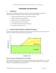
Seepage Modeling with SEEP/W - GeoStudio 2007 version 7.22
Seepage Modeling with SEEP/W - GeoStudio 2007 version 7.22

You also want an ePaper? Increase the reach of your titles
YUMPU automatically turns print PDFs into web optimized ePapers that Google loves.
Chapter 2: Numerical <strong>Modeling</strong><br />
<strong>SEEP</strong>/W<br />
It is unrealistic to dump all your information into a numerical model at the start of an analysis project and<br />
magically obtain beautiful, logical and reasonable solutions. It is vitally important to not start <strong>with</strong> this<br />
expectation. You will likely have a very unhappy modeling experience if you follow this approach.<br />
Do numerical experiments<br />
Interpreting the results of numerical models sometimes requires doing numerical experiments. This is<br />
particularly true if you are uncertain as to whether the results are reasonable. This approach also helps<br />
<strong>with</strong> understanding and learning how a particular feature operates. The idea is to set up a simple problem<br />
for which you can create a hand calculated solution.<br />
Consider the following example. You are uncertain about the results from a flux section or the meaning of<br />
a computed boundary flux. To help satisfy this lack of understanding, you could do a numerical<br />
experiment on a simple 1D case as shown in Figure 2-18. The total head difference is 1 m and the<br />
conductivity is 1 m/day. The gradient under steady state conditions is the head difference divided by the<br />
length, making the gradient 0.1. The resulting total flow through the system is the cross sectional area<br />
times the gradient which should be 0.3 m 3 /day. The flux section that goes through the entire section<br />
confirms this result. There are flux sections through Elements 16 and 18. The flow through each element<br />
is 0.1 m 3 /day, which is correct since each element represents one-third of the area.<br />
Another way to check the computed results is to look at the node information. When a head is specified,<br />
<strong>SEEP</strong>/W computes the corresponding nodal flux. In <strong>SEEP</strong>/W these are referred to as boundary flux<br />
values. The computed boundary nodal flux for the same experiment shown in Figure 2-18 on the left at<br />
the top and bottom nodes is 0.05. For the two intermediate nodes, the nodal boundary flux is 0.1 per node.<br />
The total is 0.3, the same as computed by the flux section. Also, the quantities are positive, indicating<br />
flow into the system. The nodal boundary values on the right are the same as on the left, but negative. The<br />
negative sign means flow out of the system.<br />
3<br />
2<br />
6<br />
5<br />
9<br />
8<br />
12<br />
11<br />
15<br />
3.0000e-001<br />
14<br />
18<br />
17<br />
1.0000e-001<br />
21<br />
20<br />
24<br />
23<br />
27<br />
26<br />
30<br />
29<br />
1<br />
4<br />
7<br />
10<br />
13<br />
16<br />
19<br />
22<br />
25<br />
28<br />
1.0000e-001<br />
Figure 2-18 Horizontal flow through three element section<br />
A simple numerical experiment takes only minutes to set up and run, but can be invaluable in confirming<br />
to you how the software works and in helping you interpret the results. There are many benefits: the most<br />
obvious is that it demonstrates the software is functioning properly. You can also see the difference<br />
between a flux section that goes through the entire problem versus a flux section that goes through a<br />
single element. You can see how the boundary nodal fluxes are related to the flux sections. It verifies for<br />
you the meaning of the sign on the boundary nodal fluxes. Fully understanding and comprehending the<br />
results of a simple example like this greatly helps increase your confidence in the interpretation of results<br />
from more complex problems.<br />
Page 18