Seepage Modeling with SEEP/W - GeoStudio 2007 version 7.22
Seepage Modeling with SEEP/W - GeoStudio 2007 version 7.22
Seepage Modeling with SEEP/W - GeoStudio 2007 version 7.22

You also want an ePaper? Increase the reach of your titles
YUMPU automatically turns print PDFs into web optimized ePapers that Google loves.
<strong>Seepage</strong> <strong>Modeling</strong><br />
<strong>with</strong> <strong>SEEP</strong>/W<br />
An Engineering Methodology<br />
July 2012 Edition<br />
GEO-SLOPE International Ltd.
Copyright © 2004-2012 by GEO-SLOPE International, Ltd.<br />
All rights reserved. No part of this work may be reproduced or transmitted in any<br />
form or by any means, electronic or mechanical, including photocopying,<br />
recording, or by any information storage or retrieval system, <strong>with</strong>out the prior<br />
written permission of GEO-SLOPE International, Ltd.<br />
Trademarks: GEO-SLOPE, <strong>GeoStudio</strong>, SLOPE/W, <strong>SEEP</strong>/W, SIGMA/W,<br />
QUAKE/W, CTRAN/W, TEMP/W, AIR/W and VADOSE/W are trademarks or<br />
registered trademarks of GEO-SLOPE International Ltd. in Canada and other<br />
countries. Other trademarks are the property of their respective owners.<br />
GEO-SLOPE International Ltd<br />
1400, 633 – 6 th Ave SW<br />
Calgary, Alberta, Canada T2P 2Y5<br />
E-mail: info@geo-slope.com<br />
Web: http://www.geo-slope.com
<strong>SEEP</strong>/W<br />
Table of Contents<br />
Table of Contents<br />
1 Introduction ......................................................................................... 1<br />
2 Numerical <strong>Modeling</strong>: What, Why and How ......................................... 3<br />
2.1 Introduction 3<br />
2.2 What is a numerical model? 3<br />
2.3 <strong>Modeling</strong> in geotechnical engineering 5<br />
2.4 Why model? 7<br />
Quantitative predictions ................................................................................................ 8<br />
Compare alternatives ................................................................................................... 9<br />
Identify governing parameters .................................................................................... 10<br />
Discover & understand physical process - train our thinking ..................................... 11<br />
2.5 How to model 14<br />
Make a guess ............................................................................................................. 14<br />
Simplify geometry ....................................................................................................... 16<br />
Start simple ................................................................................................................. 17<br />
Do numerical experiments .......................................................................................... 18<br />
Model only essential components .............................................................................. 19<br />
Start <strong>with</strong> estimated material properties ..................................................................... 20<br />
Interrogate the results ................................................................................................. 21<br />
Evaluate results in the context of expected results .................................................... 21<br />
Remember the real world ........................................................................................... 21<br />
2.6 How not to model 22<br />
2.7 Closing remarks 23<br />
3 Geometry and Meshing .................................................................... 25<br />
3.1 Introduction 25<br />
3.2 Geometry objects in <strong>GeoStudio</strong> 26<br />
Soil regions, points and lines ...................................................................................... 27<br />
Free points .................................................................................................................. 29<br />
Free lines .................................................................................................................... 29<br />
Interface elements on lines ......................................................................................... 31<br />
Circular openings ........................................................................................................ 33<br />
3.3 Mesh generation 34<br />
Structured mesh ......................................................................................................... 35<br />
Unstructured quad and triangle mesh ........................................................................ 35<br />
Unstructured triangular mesh ..................................................................................... 35<br />
Page i
Table of Contents<br />
<strong>SEEP</strong>/W<br />
Triangular grid regions ................................................................................................ 36<br />
Rectangular grid of quads .......................................................................................... 37<br />
3.4 Surface layers 37<br />
3.5 Joining regions 40<br />
3.6 Meshing for transient analyses 41<br />
3.7 Finite elements 42<br />
3.8 Element fundamentals 43<br />
Element nodes ............................................................................................................ 43<br />
Field variable distribution ............................................................................................ 43<br />
Element and mesh compatibility ................................................................................. 44<br />
Numerical integration .................................................................................................. 46<br />
Secondary variables ................................................................................................... 47<br />
3.9 Infinite regions 47<br />
3.10 General guidelines for meshing 49<br />
Number of elements ................................................................................................... 49<br />
Effect of drawing scale ............................................................................................... 50<br />
Mesh purpose ............................................................................................................. 50<br />
Simplified geometry .................................................................................................... 52<br />
4 Material Models and Properties ........................................................ 53<br />
4.1 Soil behavior models 53<br />
Material models in <strong>SEEP</strong>/W ....................................................................................... 53<br />
4.1 Soil water storage – water content function 54<br />
Factors affecting the volumetric water content ........................................................... 56<br />
4.2 Storage function types and estimation methods 56<br />
Estimation method 1 (grain size - Modified Kovacs) .................................................. 57<br />
Estimation method 2 (sample functions) .................................................................... 59<br />
Closed form option 1 (Fredlund and Xing, 1994) ....................................................... 60<br />
Closed form option 2 (Van Genuchten, 1980) ............................................................ 61<br />
4.3 Soil material function measurement 62<br />
Direct measurement of water content function ........................................................... 62<br />
4.4 Coefficient of volume compressibility 63<br />
4.5 Hydraulic conductivity 64<br />
4.6 Frozen ground hydraulic conductivity 66<br />
4.7 Conductivity function estimation methods 68<br />
Method 1 (Fredlund et al, 1994) ................................................................................. 68<br />
Method 2 (Green and Corey, 1971) ........................................................................... 69<br />
Page ii
<strong>SEEP</strong>/W<br />
Table of Contents<br />
Method 3 (Van Genuchten, 1980) .............................................................................. 70<br />
4.8 Interface model parameters 71<br />
4.9 Sensitivity of hydraulic results to material properties 72<br />
Changes to the air-entry value (AEV)......................................................................... 72<br />
Changes to the saturated hydraulic conductivity ........................................................ 74<br />
Changes to the slope of the VWC function ................................................................ 76<br />
Changes to the residual volumetric water content ..................................................... 78<br />
5 Boundary Conditions ........................................................................ 80<br />
5.1 Introduction 80<br />
5.2 Fundamentals 80<br />
5.3 Boundary condition locations 82<br />
Region face boundary conditions ............................................................................... 83<br />
5.4 Head boundary conditions 83<br />
Definition of total head ................................................................................................ 83<br />
Head boundary conditions on a dam .......................................................................... 85<br />
Constant pressure conditions ..................................................................................... 87<br />
Far field head conditions ............................................................................................ 87<br />
5.5 Specified boundary flows 88<br />
5.6 Sources and sinks 91<br />
5.7 <strong>Seepage</strong> faces 92<br />
5.8 Free drainage (unit gradient) 94<br />
5.9 Ground surface infiltration and evaporation 95<br />
5.10 Far field boundary conditions 97<br />
5.11 Boundary functions 98<br />
General ....................................................................................................................... 98<br />
Head versus time ........................................................................................................ 99<br />
Head versus volume ................................................................................................. 101<br />
Nodal flux Q versus time .......................................................................................... 102<br />
Unit flow rate versus time ......................................................................................... 103<br />
Modifier function ....................................................................................................... 104<br />
6 Analysis Types ................................................................................ 107<br />
6.1 Steady state 107<br />
Boundary condition types in steady state ................................................................. 108<br />
6.2 Transient 108<br />
Initial conditions ........................................................................................................ 108<br />
Drawing the initial water table .................................................................................. 110<br />
Page iii
Table of Contents<br />
<strong>SEEP</strong>/W<br />
Activation values ....................................................................................................... 110<br />
Spatial function for the initial conditions ................................................................... 111<br />
No initial condition .................................................................................................... 111<br />
6.3 Time stepping - temporal integration 111<br />
Finite element temporal integration formulation ....................................................... 112<br />
Problems <strong>with</strong> time step sizes .................................................................................. 112<br />
General rules for setting time steps .......................................................................... 113<br />
Adaptive time stepping ............................................................................................. 113<br />
6.4 Staged / multiple analyses 114<br />
6.5 Axisymmetric 114<br />
6.6 Plan view (confined aquifer only) 115<br />
7 Functions in <strong>GeoStudio</strong> .................................................................. 118<br />
7.1 Spline functions 118<br />
Slopes of spline functions ......................................................................................... 119<br />
7.2 Linear functions 120<br />
7.3 Step functions 120<br />
7.4 Closed form curve fits for water content functions 121<br />
7.5 Add-in functions 121<br />
7.6 Spatial functions 121<br />
8 Numerical Issues ............................................................................ 123<br />
8.1 Convergence 123<br />
Significant figures ..................................................................................................... 124<br />
Minimum difference .................................................................................................. 124<br />
8.2 Evaluating convergence 124<br />
Mesh view ................................................................................................................. 124<br />
Graphs ...................................................................................................................... 125<br />
Commentary ............................................................................................................. 127<br />
8.3 Under-relaxation 127<br />
8.4 Gauss integration order 127<br />
8.5 Equation solvers (direct or parallel direct) 128<br />
8.6 Time stepping 129<br />
Estimating a starting time step size .......................................................................... 129<br />
Time steps too small ................................................................................................. 129<br />
9 Flow nets, seepage forces, and exit gradients ................................ 131<br />
9.1 Flow nets 131<br />
Page iv
<strong>SEEP</strong>/W<br />
Table of Contents<br />
Equipotential lines .................................................................................................... 132<br />
Flow paths ................................................................................................................ 132<br />
Flow channels ........................................................................................................... 133<br />
Flow quantities .......................................................................................................... 135<br />
Uplift pressures ......................................................................................................... 136<br />
Limitations ................................................................................................................ 136<br />
9.2 <strong>Seepage</strong> forces 137<br />
Forces on a soil element .......................................................................................... 137<br />
9.3 Exit gradients 138<br />
Gradients .................................................................................................................. 138<br />
Critical gradients ....................................................................................................... 139<br />
Geometry considerations .......................................................................................... 139<br />
Effective stress and soil strength .............................................................................. 142<br />
Flow velocity ............................................................................................................. 143<br />
9.4 Concluding remarks 143<br />
10 Visualization of Results ................................................................... 145<br />
10.1 Transient versus steady state results 145<br />
10.2 Node and element information 145<br />
10.3 Graphing node and gauss Data 148<br />
10.4 “None” values 150<br />
10.5 Water table 150<br />
10.6 Isolines 151<br />
10.7 Projecting Gauss point values to nodes 151<br />
10.8 Contours 152<br />
10.9 Animation in <strong>GeoStudio</strong> 153<br />
10.10 Velocity vectors and flow paths 153<br />
Calculating gradients and velocities ......................................................................... 153<br />
Velocity vectors ........................................................................................................ 154<br />
Flow paths ................................................................................................................ 154<br />
10.11 Flux sections 155<br />
Flux section theory ................................................................................................... 156<br />
Flux section application ............................................................................................ 157<br />
11 <strong>Modeling</strong> Tips and Tricks ................................................................ 159<br />
11.1 Introduction 159<br />
11.2 Problem engineering units 159<br />
11.3 Flux section location 160<br />
Page v
Table of Contents<br />
<strong>SEEP</strong>/W<br />
11.4 Drain flux values 161<br />
11.5 Unit flux versus total flux? 162<br />
11.6 Flow above phreatic line 163<br />
11.7 Pressure boundary <strong>with</strong> depth 164<br />
11.8 Summing graphed data 165<br />
12 Illustrative Examples ....................................................................... 169<br />
13 Theory ............................................................................................. 171<br />
13.1 Darcy’s law 171<br />
13.2 Partial differential water flow equations 171<br />
13.3 Finite element water flow equations 173<br />
13.4 Temporal integration 174<br />
13.5 Numerical integration 175<br />
13.6 Hydraulic conductivity matrix 177<br />
13.7 Mass matrix 178<br />
13.8 Flux boundary vector 179<br />
13.9 Density-dependent flow 182<br />
14 Appendix A: Interpolating Functions ............................................... 185<br />
14.1 Coordinate systems 185<br />
14.2 Interpolating functions 187<br />
Field variable model ................................................................................................. 187<br />
Interpolation function derivatives .............................................................................. 188<br />
References ............................................................................................... 191<br />
Index 196<br />
Page vi
<strong>SEEP</strong>/W<br />
Chapter 1: Introduction<br />
1 Introduction<br />
The flow of water through soil is one of the fundamental processes in geotechnical and geoenvironmental<br />
engineering. In fact, there would little need for geotechnical engineering if water were not<br />
present in the soil. This is a nonsensical statement: if there were no water in the soil, there would be no<br />
way to sustain an ecosystem, no humans on earth and no need for geotechnical and geo-environmental<br />
engineering. However, the statement does highlight the importance of water in working <strong>with</strong> soil and<br />
rock.<br />
Flow quantity is a key parameter in quantifying seepage losses from a reservoir or indentifying a potential<br />
water supply for domestic or industrial use. Pore-pressures associated <strong>with</strong> groundwater flow are of<br />
particular concern in geotechnical engineering. The pore-water pressure, whether positive or negative, is<br />
an integral component of the stress state <strong>with</strong>in the soil and consequently has a direct bearing on the shear<br />
strength and volume change behavior of soil. Research in the last few decades has highlighted the<br />
importance of moisture flow dynamics in unsaturated surficial soils as it relates to the design of soil<br />
covers.<br />
Historically, analyses of groundwater flow have focused on flow in saturated soils and flow problems<br />
were typically categorized as being confined or unconfined situations. Flow beneath a structure would be<br />
a confined flow problem, while flow through a homogeneous embankment would be an unconfined flow<br />
problem. Unconfined flow problems were often considered more difficult to analyze because the<br />
determination of the location of the phreatic surface (i.e., the transition from positive to negative pore<br />
water pressures) was integral to the analyses. The phreatic surface was considered an upper boundary and<br />
any flow that may have existed in the capillary zone above the phreatic line was ignored.<br />
It is no longer acceptable to simply ignore the movement of water in unsaturated soils above the phreatic<br />
surface. Not only does it ignore an important component of moisture flow in soils, but it greatly limits the<br />
types of problems that can be analyzed. It is central to the analysis of problems involving infiltration and<br />
moisture redistribution in the vadose zone. Transient flow problems such as the advance of a wetting<br />
front <strong>with</strong>in an earth structure after rapid filling are typical examples of situations in which it is<br />
impossible to simulate field behavior <strong>with</strong>out correctly considering the physics of flow through<br />
unsaturated soils. Fortunately, it is no longer necessary to ignore the unsaturated zone. With the help of<br />
this document and the associated software, flow through unsaturated soils can be incorporated into<br />
numerical models so that almost any kind of seepage problem can be analyzed.<br />
In general, all water flow is driven by energy gradients associated <strong>with</strong> the total head of water as<br />
represented by the components of pressure head (or pore water pressure) and elevation. The term<br />
seepage often is used to describe flow problems in which the dominant driving energy is gravity, such as<br />
a case in which seepage losses occur from a reservoir to a downstream exit point. In other situations such<br />
as consolidation, the primary driving energy may be associated <strong>with</strong> the creation of excess pore-water<br />
pressures as a result of external loading. However, both of these situations can all be described by a<br />
common set of mathematical equations describing the water movement. As a result, the formulation used<br />
to analyze seepage problems can also be used to analyze the dissipation of excess pore-water pressures<br />
resulting from changes in stress conditions. In the context of the discussions and examples in this<br />
document and in using the <strong>SEEP</strong>/W software, the term seepage is used to describe all movement of water<br />
through soil regardless of the creation or source of the driving energy or whether the flow is through<br />
saturated or unsaturated soils.<br />
Simulating the flow of water through soil <strong>with</strong> a numerical model can be very complex. Natural soil<br />
deposits are generally highly heterogeneous and non-isotropic. In addition, boundary conditions often<br />
change <strong>with</strong> time and cannot always be defined <strong>with</strong> certainty at the beginning of an analysis. In some<br />
Page 1
Chapter 1: Introduction<br />
<strong>SEEP</strong>/W<br />
cases the correct boundary conditions themselves are part of the outcome from the solution. Furthermore,<br />
when a soil becomes unsaturated, the coefficient of permeability or hydraulic conductivity becomes a<br />
function of the negative pore-water pressure in the soil. Since the pore-water pressure is related to the<br />
primary unknown (total head) and must be computed, iterative numerical techniques are required to<br />
compute the appropriate combination of pore-water pressure and the material property. This is referred to<br />
as a non-linear problem. These complexities make it necessary to use some form of numerical analysis to<br />
analyze seepage problems for all but the simplest cases.<br />
While part of this document is about using <strong>SEEP</strong>/W to do seepage analyses, it is also about general<br />
numerical modeling techniques. Numerical modeling, like most things in life, is a skill that needs to be<br />
acquired. It is nearly impossible to pick up a tool like <strong>SEEP</strong>/W and immediately become an effective<br />
modeler. Effective numerical modeling requires some careful thought and planning and it requires a good<br />
understanding of the underlying fundamental theory and concepts. Steps in the analyses such as creating<br />
the finite element mesh and applying boundary conditions are not entirely intuitive at first. Time and<br />
practice are required to become comfortable <strong>with</strong> these aspects of numerical modeling.<br />
A large portion of this book focuses on general guidelines for conducting effective analyses using a<br />
numerical model. Chapter 2, Numerical <strong>Modeling</strong>: What, Why and How, is devoted exclusively to<br />
discussions on this topic. The general principles discussed apply to all numerical modeling situations, but<br />
are used in the context of seepage analyses in this document.<br />
Broadly speaking, there are three main parts to a finite element analysis. The first is creating the<br />
numerical domain, including the selection of an appropriate geometry and creating the discretized mesh.<br />
The second part requires the specification of material properties to the various sub-regions of the domain.<br />
The third is the specification of the appropriate boundary conditions. Separate chapters have been<br />
devoted to each of these three key components <strong>with</strong>in this document.<br />
The analysis of flow through saturated and unsaturated soils using numerical models is a highly nonlinear<br />
problem that requires iterative techniques to obtain solutions. Numerical convergence is<br />
consequently a key issue. Also, the temporal integration scheme, which is required for a transient<br />
analysis, is affected by time step size relative to element size and material properties. These and other<br />
numerical considerations are discussed in Chapter 8, Numerical Issues.<br />
Chapter 11, <strong>Modeling</strong> Tips and Tricks, should be consulted to see if there are simple techniques that can<br />
be used to improve your general modeling method. You will also gain more confidence and develop a<br />
deeper understanding of finite element methods, <strong>SEEP</strong>/W conventions and data results.<br />
Chapter 12 has been dedicated to presenting examples in a brief, introductory format. The details of all<br />
examples along <strong>with</strong> the actual project files are available on a separate DVD or by download from our<br />
web site. You should scan over this chapter and see the many verification examples and case study<br />
examples to understand the capabilities of the software.<br />
Chapter 13, Theory, is dedicated to theoretical issues associated <strong>with</strong> the finite element solution of the<br />
partial differential flow equation for saturated and unsaturated soils. Additional finite element numerical<br />
details regarding interpolating functions and infinite elements are given in Appendix A, Interpolating<br />
Functions.<br />
In general, this book is not a “how to use <strong>SEEP</strong>/W” manual. It is a book about how to model. It also<br />
describes how to engineer seepage problems using a powerful calculator; <strong>SEEP</strong>/W. Details of how to use<br />
the various program commands and features of <strong>SEEP</strong>/W are given in the online help inside the software.<br />
Page 2
<strong>SEEP</strong>/W<br />
Chapter 2: Numerical <strong>Modeling</strong><br />
2 Numerical <strong>Modeling</strong>: What, Why and How<br />
2.1 Introduction<br />
The unprecedented computing power now available has resulted in advanced software products for<br />
engineering and scientific analysis. The ready availability and ease-of-use of these products makes it<br />
possible to use powerful techniques such as a finite element analysis in engineering practice. These<br />
analytical methods have now moved from being research tools to application tools. This has opened a<br />
whole new world of numerical modeling.<br />
Software tools such as <strong>SEEP</strong>/W do not inherently lead to good results. While the software is an extremely<br />
powerful calculator, obtaining useful and meaningful results from this useful tool depends on the<br />
guidance provided by the user. It is the users’ understanding of the input and their ability to interpret the<br />
results that make it such a powerful tool. In summary, the software does not do the modeling, the user<br />
does the modeling. The software only provides the ability to do highly complex computations that are not<br />
otherwise humanly possible. In a similar manner, modern day spreadsheet software programs can be<br />
immensely powerful as well, but obtaining useful results from a spreadsheet depends on the user. It is the<br />
user’s ability to guide the analysis process that makes it a powerful tool. The spreadsheet can do all the<br />
mathematics, but it is the user’s ability to take advantage of the computing capability that leads to<br />
something meaningful and useful. The same is true <strong>with</strong> finite element analysis software such as<br />
<strong>SEEP</strong>/W.<br />
Numerical modeling is a skill that is acquired <strong>with</strong> time and experience. Simply acquiring a software<br />
product does not immediately make a person a proficient modeler. Time and practice are required to<br />
understand the techniques involved and learn how to interpret the results.<br />
Numerical modeling as a field of practice is relatively new in geotechnical engineering and, consequently,<br />
there is a lack of understanding about what numerical modeling is, how modeling should be approached<br />
and what to expect from it. A good understanding of these basic issues is fundamental to conducting<br />
effective modeling. Basic questions such as, What is the main objective of the analysis?, What is the main<br />
engineering question that needs to answered? and, What is the anticipated result?, need to be decided<br />
before starting to use the software. Using the software is only part of the modeling exercise. The<br />
associated mental analysis is as important as clicking the buttons in the software.<br />
This chapter discusses the “what”, “why” and “how” of the numerical modeling process and presents<br />
guidelines on the procedures that should be followed in good numerical modeling practice.<br />
2.2 What is a numerical model?<br />
A numerical model is a mathematical simulation of a real physical process. <strong>SEEP</strong>/W is a numerical model<br />
that can mathematically simulate the real physical process of water flowing through a particulate medium.<br />
Numerical modeling is purely mathematical and in this sense is very different than scaled physical<br />
modeling in the laboratory or full-scaled field modeling.<br />
Rulon (1985) constructed a scale model of a soil slope <strong>with</strong> a less permeable layer embedded <strong>with</strong>in the<br />
slope and then sprinkled water on the crest to simulate infiltration or precipitation. Instruments were<br />
inserted into the soil through the side walls to measure the pore-water pressures at various points. The<br />
results of her experiment are shown in Figure 2-1. <strong>Modeling</strong> Rulon’s laboratory experiment <strong>with</strong> <strong>SEEP</strong>/W<br />
gives the results presented in Figure 2-2, which are almost identical to the original laboratory<br />
measurements. The positions of the equipotential lines are somewhat different, but the position of the<br />
water table is the same. In both cases there are two seepage exit areas on the slope, which is the main<br />
Page 3
Chapter 2: Numerical <strong>Modeling</strong><br />
<strong>SEEP</strong>/W<br />
important observation in this case. (Details of the <strong>SEEP</strong>/W analysis of this case are presented in Chapter<br />
12, Illustrative Examples).<br />
1.0<br />
0.9<br />
0.8<br />
Figure 2-1 Rulon’s laboratory scaled model results<br />
Z (m)<br />
0.7<br />
0.6<br />
0.5<br />
0.4<br />
Fine Sand<br />
0.3<br />
0.2<br />
0.1<br />
0.0<br />
0.0 0.2 0.4 0.6 0.8 1.0 1.2 1.4 1.6 1.8 2.0 2.2 2.4<br />
Figure 2-2 <strong>SEEP</strong>/W analysis of Rulon’s laboratory model<br />
The fact that mathematics can be used to simulate real physical processes is one of the great wonders of<br />
the universe. Perhaps physical processes follow mathematical rules, or mathematics has evolved to<br />
describe physical processes. Obviously, we do not know which came first, nor does it really matter.<br />
Regardless of how the relationship developed, the fact that we can use mathematics to simulate physical<br />
processes leads to developing a deeper understanding of physical processes. It may even allow for<br />
understanding or discovering previously unknown physical processes.<br />
Numerical modeling has many advantages over physical modeling. The following are some of the more<br />
obvious advantages.<br />
X (m)<br />
Numerical models can be set up very quickly relative to physical models. Physical models may<br />
take months to construct while a numerical model can be constructed in minutes, hours or<br />
days.<br />
A physical model is usually limited to a narrow set of conditions. A numerical model can be used<br />
to investigate a wide variety of different scenarios.<br />
Page 4
<strong>SEEP</strong>/W<br />
Chapter 2: Numerical <strong>Modeling</strong><br />
Numerical models have no difficulty accounting for gravity. Gravity cannot be scaled, which is a<br />
limitation <strong>with</strong> laboratory modeling. A centrifuge is often required to overcome this<br />
limitation.<br />
With numerical modeling, there is no danger of physical harm to personnel. Physical modeling<br />
sometimes involves heavy equipment and worker safety is consequently a concern.<br />
Numerical modeling provides information and results at any location <strong>with</strong>in the cross-section.<br />
Physical modeling only provides external visual responses and data at discrete instrumented<br />
points.<br />
Numerical models can accommodate a wide variety of boundary conditions, whereas physical<br />
models are often limited in the types of boundary conditions possible.<br />
It would be wrong to think that numerical models do not have limitations. Associated <strong>with</strong> seepage flow<br />
there may also be temperature changes, volume changes and perhaps chemical changes. Including all<br />
these processes in the same formulation is not possible, as the mathematics involved simply become too<br />
complex. In addition, it is not possible to mathematically describe a constitutive relationship, due to its<br />
complexity. Some of these difficulties can and will be overcome <strong>with</strong> greater and faster computer<br />
processing power. It is important to understand that numerical modeling products like <strong>SEEP</strong>/W will have<br />
limitations that are related to the current capability of hardware or integral to the formulation of the<br />
software, since it was developed to consider specific conditions. <strong>SEEP</strong>/W is formulated only for flow that<br />
follows Darcy’s Law. Near the ground surface moisture may leave the ground as vapor. This component<br />
is not included in the <strong>SEEP</strong>/W formulation, like it is in another product called VADOSE/W.<br />
Consequently, <strong>SEEP</strong>/W has limitations when it comes to modeling moisture leaving the system at the<br />
ground surface. A real physical model would not have this type of limitation.<br />
The important point to remember is that the mathematical formulations implemented in software like<br />
<strong>SEEP</strong>/W result in a very powerful and versatile means of simulating real physical processes.<br />
“A mathematical model is a replica of some real-world object or system. It is an attempt to take our understanding of<br />
the process (conceptual model) and translate it into mathematical terms.” National Research Council Report (1990).<br />
2.3 <strong>Modeling</strong> in geotechnical engineering<br />
The role and significance of analysis and numerical modeling in geotechnical engineering has been<br />
vividly illustrated by Professor John Burland, Imperial College, London (UK). In 1987 Professor Burland<br />
presented what is known as the Nash Lecture. The title of the lecture was “The Teaching of Soil<br />
Mechanics – a Personal View”. In this lecture he advocated that geotechnical engineering consists of<br />
three fundamental components: the ground profile, the soil behavior and modeling. He represented these<br />
components as the apexes of a triangle, as illustrated in Figure 2-3. This has come to be known as the<br />
Burland triangle (Burland, 1987; Burland, 1996).<br />
Page 5
Chapter 2: Numerical <strong>Modeling</strong><br />
<strong>SEEP</strong>/W<br />
Ground<br />
profile<br />
Empiricism,<br />
Precedent<br />
Soil<br />
behaviour<br />
<strong>Modeling</strong><br />
The soil mechanics triangle<br />
Figure 2-3 The Burland triangle (after Burland 1996)<br />
The soil behavior component includes laboratory tests, in situ tests and field measurements. The ground<br />
profile component basically involves site characterization: defining and describing the site conditions.<br />
<strong>Modeling</strong> may be conceptual, analytical or physical.<br />
Of great significance is that, in Burland’s view, all three components need to be tied together by<br />
empiricism and precedent. This is the part inside the triangle.<br />
The Burland triangle idea has been widely discussed and referred to by others since it was first presented.<br />
An article on this topic was presented in an issue of Ground Engineering (Anon. 1999). Morgenstern<br />
(2000) discussed this at some length in his keynote address titled “Common Ground” at the GeoEng2000<br />
Conference in Melbourne Australia in 2000. With all the discussion, the triangle has been enhanced and<br />
broadened somewhat, as shown in Figure 2-4.<br />
One important additional feature has been to consider all the connecting arrows between the components<br />
as pointing in both directions. This simple addition highlights the fact that each part is distinct yet related<br />
to all the other parts.<br />
The Burland triangle vividly illustrates the importance of modeling in geotechnical engineering.<br />
Characterizing the field conditions and making measurements of behavior is not sufficient. Ultimately, it<br />
is necessary to do some analysis of the field information and soil properties to complete the triangle.<br />
As Burland pointed out, modeling may be conceptual, analytical or physical. However, <strong>with</strong> the<br />
computing power and software tools now available, modeling often refers to numerical modeling.<br />
Accepting that modeling primarily refers to numerical modeling, the Burland triangle shows the<br />
importance that numerical modeling has in geotechnical engineering.<br />
Page 6
<strong>SEEP</strong>/W<br />
Chapter 2: Numerical <strong>Modeling</strong><br />
Genesis / geology<br />
Ground<br />
Profile<br />
Site investigation,<br />
ground description<br />
Empiricism,<br />
precedent,<br />
experience,<br />
risk management<br />
Soil<br />
Behaviour<br />
<strong>Modeling</strong><br />
Lab / field testing,<br />
observation,<br />
measurement<br />
Idealization followed by<br />
evaluation. Conceptual<br />
or physical modeling,<br />
analytical modeling<br />
Figure 2-4 The enhanced Burland triangle (after Anon. 1999)<br />
Making measurements and characterizing site conditions is often time consuming and expensive. This is<br />
also true <strong>with</strong> modeling, if done correctly. A common assumption is that the numerical modeling<br />
component is only a small component that should be undertaken at the end of a project, and that it can be<br />
done simply and quickly. This is somewhat erroneous. Good numerical modeling, as we will see later in<br />
the section in more detail, takes time and requires careful planning in the same manner that it takes time<br />
and planning to collect field measurements and adequately characterize site conditions.<br />
Considering the importance of modeling that the Burland triangle suggests for geotechnical engineering,<br />
it is prudent that we do the modeling carefully and <strong>with</strong> a complete understanding of the modeling<br />
processes. This is particularly true <strong>with</strong> numerical modeling. The purpose of this book is to assist <strong>with</strong><br />
this aspect of geotechnical engineering.<br />
2.4 Why model?<br />
The first reaction to the question, “why model?” seems rather obvious. The objective is to analyze the<br />
problem. Upon more thought, the answer becomes increasingly complex. Without a clear understanding<br />
of the reason for modeling or identifying what the modeling objectives are, numerical modeling can lead<br />
to a frustrating experience and uncertain results. As we will see in more detail in the next section, it is<br />
wrong to set up the model, calculate a solution and then try to decide what the results mean. It is<br />
important to decide at the outset the reason for doing the modeling. What is the main objective and what<br />
is the question that needs to be answered?<br />
The following points are some of the main reasons for modeling, from a broad, high level perspective. We<br />
model to:<br />
make quantitative predictions,<br />
compare alternatives,<br />
identify governing parameters, and<br />
understand processes and train our thinking.<br />
Page 7
Chapter 2: Numerical <strong>Modeling</strong><br />
<strong>SEEP</strong>/W<br />
Quantitative predictions<br />
Most engineers, when asked why they want to do some modeling, will say that they want to make a<br />
prediction. They want to predict the seepage quantity, for example, or the time for a contaminant to travel<br />
from the source to a seepage discharge point, or the time required from first filling a reservoir until<br />
steady-state seepage conditions have been established in the embankment dam. The desire is to say<br />
something about future behavior or performance.<br />
Making quantitative predictions is a legitimate reason for doing modeling. Unfortunately, it is also the<br />
most difficult part of modeling, since quantitative values are often directly related to the material<br />
properties. The quantity of seepage, for example, is in large part controlled by the hydraulic conductivity<br />
and, as a result, changing the hydraulic conductivity by an order of magnitude will usually change the<br />
computed seepage quantity by an order of magnitude. The accuracy of quantitative prediction is directly<br />
related to the accuracy of the hydraulic conductivity specified. Unfortunately, for a heterogeneous profile,<br />
there is not a large amount of confidence about how precisely the hydraulic conductivity can be specified.<br />
Sometimes defining the hydraulic conductivity <strong>with</strong>in an order of magnitude is considered reasonable.<br />
The confidence you have defining the hydraulic conductivity depends on many factors, but the general<br />
difficulty of defining this soil parameter highlights the difficulty of undertaking modeling to make<br />
quantitative predictions.<br />
Carter et al. (2000) presented the results of a competition conducted by the German Society for<br />
Geotechnics. Packages of information were distributed to consulting engineers and university research<br />
groups. The participants were asked to predict the lateral deflection of a tie-back shoring wall for a deep<br />
excavation in Berlin. During construction, the actual deflection was measured <strong>with</strong> inclinometers. Later<br />
the predictions were compared <strong>with</strong> the actual measurements. Figure 2-5 shows the best eleven submitted<br />
predictions. Other predictions were submitted, but were considered unreasonable and consequently not<br />
included in the summary.<br />
There are two heavy dark lines superimposed on Figure 2-5. The dashed line on the right represents the<br />
inclinometer measurements uncorrected for any possible base movement. It is likely the base of the<br />
inclinometer moved together <strong>with</strong> the base of the wall. Assuming the inclinometer base moved about<br />
10 mm, the solid heavy line in Figure 2-5 has been shifted to reflect the inclinometer base movement.<br />
At first glance one might quickly conclude that the agreement between prediction and actual lateral<br />
movement is very poor, especially since there appears to be a wide scatter in the predictions. This<br />
exercise might be considered as an example of our inability to make accurate quantitative predictions.<br />
However, a closer look at the results reveals a picture that is not so bleak. The depth of the excavation is<br />
32 m. The maximum predicted lateral movement is just over 50 mm or 5 cm. This is an extremely small<br />
amount of movement over the length of the wall – certainly not big enough to be visually noticeable.<br />
Furthermore, the actual measurements, when corrected for base movement fall more or less in the middle<br />
of the predictions. Most important to consider are the trends presented by many of the predicted results.<br />
Many of them predict a deflected shape similar to the actual measurements. In other words, the<br />
predictions simulated the correct relative response of the wall.<br />
Consequently, we can argue that our ability to make accurate predictions is poor, but we can also argue<br />
that the predictions are amazingly good. The predictions fall on either side of the measurements and the<br />
deflected shapes are correct. In the end, the modeling provided a correct understanding of the wall<br />
behavior, which is more than enough justification for doing the modeling, and may be the greatest benefit<br />
of numerical modeling, as we will see in more detail later.<br />
Page 8
<strong>SEEP</strong>/W<br />
Chapter 2: Numerical <strong>Modeling</strong><br />
Deflection (mm)<br />
-60 -50 -40 -30 -20 -10 0 1<br />
0<br />
4<br />
8<br />
12<br />
16<br />
20<br />
Depth below surface (m)<br />
24<br />
computed<br />
measured<br />
28<br />
Figure 2-5 Comparison of predicted and measured lateral movements of a shoring wall<br />
(after Carter et al, 2000)<br />
Numerical modeling is sometimes dismissed as being useless due to the difficulty <strong>with</strong> defining material<br />
properties. There are, however, other reasons for doing numerical modeling. If some of the other<br />
objectives of numerical modeling are completed first, then quantitative predictions often have more value<br />
and meaning. Once the physics and mechanisms are completely understood, quantitative predictions can<br />
be made <strong>with</strong> a great deal more confidence and are not nearly as useless as first thought, regardless of our<br />
inability to accurately define material properties.<br />
Compare alternatives<br />
32<br />
-60 -50 -40 -30 -20 -10 0 1<br />
Numerical modeling is useful for comparing alternatives. Keeping everything else the same and changing<br />
a single parameter makes it a powerful tool to evaluate the significance of individual parameters. For<br />
modeling alternatives and conducting sensitivity studies it is not all that important to accurately define<br />
some material properties. All that is of interest is the change between simulations.<br />
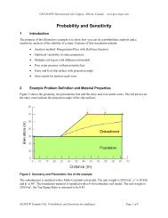
Consider the example of a cut-off wall beneath a structure. With <strong>SEEP</strong>/W it is easy to examine the<br />
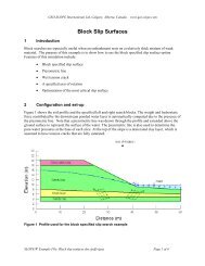
benefits obtained by changing the length of the cut-off. Consider two cases <strong>with</strong> different cut-off depths<br />
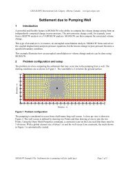
to assess the difference in uplift pressures underneath the structure. Figure 2-6 shows the analysis when<br />
the cutoff is 10 feet deep. The pressure drop and uplift pressure along the base are shown in the left graph<br />
in Figure 2-7. The drop across the cutoff is from 24 to 18 feet of pressure head. The results for a 20-foot<br />
cutoff are shown in Figure 2-7 on the right side. Now the drop across the cutoff is from 24 to about 15<br />
feet of pressure head. The uplift pressures at the downstream toe are about the same.<br />
The actual computed values are not of significance in the context of this discussion. It is an example of<br />
how a model such as <strong>SEEP</strong>/W can be used to quickly compare alternatives. Secondly, this type of<br />
Page 9
Chapter 2: Numerical <strong>Modeling</strong><br />
<strong>SEEP</strong>/W<br />
analysis can be done <strong>with</strong> a rough estimate of the conductivity, since in this case the pressure distributions<br />
will be unaffected by the conductivity assumed. There would be no value in carefully defining the<br />
conductivity to compare the base pressure distributions.<br />
We can also look at the change in flow quantities. The absolute flow quantity may not be all that accurate,<br />
but the change resulting from various cut-off depths will be of value. The total flux is 6.26 x 10 -3 ft 3 /s for<br />
the 10-foot cutoff and 5.30 x 10 -3 ft 3 /s for the 20-foot cutoff, only about a 15 percent difference.<br />
A<br />
6.2592e-003<br />
Figure 2-6 <strong>Seepage</strong> analysis <strong>with</strong> a cutoff<br />
25<br />
Cutoff 10 feet<br />
25<br />
Cutoff - 20 feet<br />
Pressure Head - feet<br />
20<br />
15<br />
10<br />
5<br />
Pressure Head - feet<br />
20<br />
15<br />
10<br />
5<br />
0<br />
30 50 70 90 110<br />
0<br />
30 50 70 90 110<br />
Distance - feet<br />
Distance - feet<br />
Figure 2-7 Uplift pressure distributions along base of structure<br />
Identify governing parameters<br />
Numerical models are useful for identifying critical parameters in a design. Consider the performance of a<br />
soil cover over waste material. What is the most important parameter governing the behavior of the<br />
cover? Is it the precipitation, the wind speed, the net solar radiation, plant type, root depth or soil type?<br />
Running a series of VADOSE/W simulations, keeping all variables constant except for one makes it<br />
possible to identify the governing parameter. The results can be presented as a tornado plot such as shown<br />
in Figure 2-8.<br />
Once the key issues have been identified, further modeling to refine a design can concentrate on the main<br />
issues. If, for example, the vegetative growth is the main issue then efforts can be concentrated on what<br />
needs to be done to foster the plant growth.<br />
Page 10
<strong>SEEP</strong>/W<br />
Chapter 2: Numerical <strong>Modeling</strong><br />
Base Case<br />
thinner<br />
Thickness<br />
of Growth Medium<br />
high<br />
low<br />
bare surface<br />
Transpiration<br />
low<br />
deep<br />
high<br />
shallow<br />
Hydraulic Conductivity<br />
of Compacted Layer<br />
Root Depth<br />
low<br />
high<br />
Hydraulic Conductivity<br />
of Growth Medium<br />
Decreasing<br />
Net Percolation<br />
Increasing<br />
Net Percolation<br />
Figure 2-8 Example of a tornado plot (O’Kane, 2004)<br />
Discover & understand physical process - train our thinking<br />
One of the most powerful aspects of numerical modeling is that it can help us to understand physical<br />
processes in that it helps to train our thinking. A numerical model can either confirm our thinking or help<br />
us to adjust our thinking if necessary.<br />
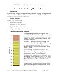
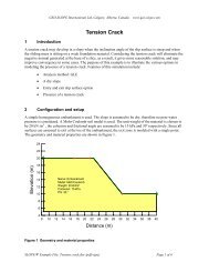
To illustrate this aspect of numerical modeling, consider the case of a multilayered earth cover system<br />
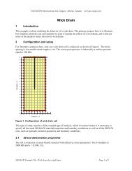
such as the two possible cases shown in Figure 2-9. The purpose of the cover is to reduce the infiltration<br />
into the underlying waste material. The intention is to use the earth cover layers to channel any infiltration<br />
downslope into a collection system. It is known that both a fine and a coarse soil are required to achieve<br />
this. The question is, should the coarse soil lie on top of the fine soil or should the fine soil overlay the<br />
coarse soil? Intuitively it would seem that the coarse material should be on top; after all, it has the higher<br />
conductivity. <strong>Modeling</strong> this situation <strong>with</strong> <strong>SEEP</strong>/W, which handles unsaturated flow, can answer this<br />
question and verify if our thinking is correct.<br />
For unsaturated flow, it is necessary to define a hydraulic conductivity function: a function that describes<br />
how the hydraulic conductivity varies <strong>with</strong> changes in suction (negative pore-water pressure = suction).<br />
Chapter 4, Material Properties, describes in detail the nature of the hydraulic conductivity (or<br />
permeability) functions. For this example, relative conductivity functions such as those presented in<br />
Figure 2-10 are sufficient. At low suctions (i.e., near saturation), the coarse material has a higher<br />
hydraulic conductivity than the fine material, which is intuitive. At high suctions, the coarse material has<br />
the lower conductivity, which often appears counterintuitive. For a full explanation of this relationship,<br />
refer to Chapter 4, Materials Properties. For this example, accept that at high suctions the coarse material<br />
is less conductive than the fine material.<br />
Page 11
Chapter 2: Numerical <strong>Modeling</strong><br />
<strong>SEEP</strong>/W<br />
Fine<br />
Coarse<br />
Material to be<br />
protected<br />
OR<br />
Coarse<br />
Fine<br />
Material to be<br />
protected<br />
Figure 2-9 Two possible earth cover configurations<br />
1.00E-04<br />
Conductivity<br />
1.00E-05<br />
1.00E-06<br />
1.00E-07<br />
1.00E-08<br />
Coarse<br />
Fine<br />
1.00E-09<br />
1.00E-10<br />
1 10 100 1000<br />
Suction<br />
Figure 2-10 Hydraulic conductivity functions<br />
After conducting various analyses and trial runs <strong>with</strong> varying rates of surface infiltration, it becomes<br />
evident that the behavior of the cover system is dependent on the infiltration rate. At low infiltration rates,<br />
the effect of placing the fine material over the coarse material results in infiltration being drained laterally<br />
through the fine layer, as shown in Figure 2-11. This accomplishes the design objective of the cover. If<br />
the precipitation rate becomes fairly intensive, then the infiltration drops through the fine material and<br />
drains laterally <strong>with</strong>in the lower coarse material as shown in Figure 2-12. The design of fine soil over<br />
coarse soil may work, but only in arid environments. The occasional cloud burst may result in significant<br />
water infiltrating into the underlying coarse material, which may result in increased seepage into the<br />
waste. This may be a tolerable situation for short periods of time. If most of the time precipitation is<br />
modest, the infiltration will be drained laterally through the upper fine layer into a collection system.<br />
So, for an arid site the best solution is to place the fine soil on top of the coarse soil. This is contrary to<br />
what one might expect at first. The first reaction may be that something is wrong <strong>with</strong> the software, but it<br />
may be that our understanding of the process and our general thinking is flawed.<br />
A closer examination of the conductivity functions provides a logical explanation. The software is correct<br />
and provides the correct response given the input parameters. Consider the functions in Figure 2-13.<br />
When the infiltration rate is large, the negative water pressures or suctions will be small. As a result, the<br />
Page 12
<strong>SEEP</strong>/W<br />
Chapter 2: Numerical <strong>Modeling</strong><br />
conductivity of the coarse material is higher than the finer material. If the infiltration rates become small,<br />
the suctions will increase (water pressure becomes more negative) and the unsaturated conductivity of the<br />
finer material becomes higher than the coarse material. Consequently, under low infiltration rates it is<br />
easier for the water to flow through the fine, upper layer soil than through the lower more coarse soil.<br />
Fine<br />
Coarse<br />
Low to modest rainfall rates<br />
Figure 2-11 Flow di<strong>version</strong> under low infiltration<br />
Fine<br />
Coarse<br />
Intense rainfall rates<br />
Figure 2-12 Flow di<strong>version</strong> under high infiltration<br />
This type of analysis is a good example where the ability to utilize a numerical model greatly assists our<br />
understanding of the physical process. The key is to think in terms of unsaturated conductivity as opposed<br />
to saturated conductivities.<br />
Numerical modeling can be crucial in leading us to the discovery and understanding of real physical<br />
processes. In the end the model either has to conform to our mental image and understanding or our<br />
understanding has to be adjusted.<br />
Page 13
Chapter 2: Numerical <strong>Modeling</strong><br />
<strong>SEEP</strong>/W<br />
1.00E-04<br />
Conductivity<br />
1.00E-05<br />
1.00E-06<br />
1.00E-07<br />
1.00E-08<br />
1.00E-09<br />
Intense<br />
Rainfall<br />
Coarse<br />
Fine<br />
Low to Modest<br />
Rainfall<br />
1.00E-10<br />
1 10 100 1000<br />
Suction<br />
Figure 2-13 Conductivities under low and intense infiltration<br />
This is a critical lesson in modeling and the use of numerical models in particular. The key advantage of<br />
modeling, and in particular the use of computer modeling tools, is the capability it has to enhance<br />
engineering judgment, not the ability to enhance our predictive capabilities. While it is true that<br />
sophisticated computer tools greatly elevated our predictive capabilities relative to hand calculations,<br />
graphical techniques, and closed-form analytical solutions, still, prediction is not the most important<br />
advantage these modern tools provide. Numerical modeling is primarily about ‘process’ - not about<br />
prediction.<br />
“The attraction of ... modeling is that it combines the subtlety of human judgment <strong>with</strong> the power of the digital<br />
computer.” Anderson and Woessner (1992).<br />
2.5 How to model<br />
Numerical modeling involves more than just acquiring a software product. Running and using the<br />
software is an essential ingredient, but it is a small part of numerical modeling. This section talks about<br />
important concepts in numerical modeling and highlights important components in good modeling<br />
practice.<br />
Make a guess<br />
Generally, careful planning is involved when undertaking a site characterization or making measurements<br />
of observed behavior. The same careful planning is required for modeling. It is inappropriate to acquire a<br />
software product, input some parameters, obtain some results, and then decide what to do <strong>with</strong> the results<br />
or struggle to decide what the results mean. This approach usually leads to an unhappy experience and is<br />
often a meaningless exercise.<br />
Good modeling practice starts <strong>with</strong> some planning. If at all possible, you should form a mental picture of<br />
what you think the results will look like. Stated another way, we should make a rough guess at the<br />
solution before starting to use the software. Figure 2-14 shows a very quick hand sketch of a flow net. It<br />
is very rough, but it gives us an idea of what the solution should look like.<br />
Page 14
<strong>SEEP</strong>/W<br />
Chapter 2: Numerical <strong>Modeling</strong><br />
From the rough sketch of a flow net, we can also get an estimate of the flow quantity. The amount of flow<br />
can be approximated by the ratio of flow channels to equipotential drops multiplied by the conductivity<br />
and the total head drop. For the sketch in Figure 2-14 the number of flow channels is 3, the number of<br />
equipotential drops is 9 and the total head drop is 5 m. Assume a hydraulic conductivity of K = 0.1 m/day.<br />
A rough estimate of the flow quantity then is (5 x 0.1 x 3)/ 9, which is between 0.1 and 0.2 m 3 / day. The<br />
<strong>SEEP</strong>/W computed flow is 0.1427 m 3 /day and the equipotential lines are as shown in Figure 2-15.<br />
Figure 2-14 Hand sketch of flow net for cutoff below dam<br />
1.4272e-001<br />
Figure 2-15 <strong>SEEP</strong>/W results compared to hand sketch estimate<br />
The rough flow net together <strong>with</strong> the estimated flow quantity can now be used to judge the <strong>SEEP</strong>/W<br />
results. If there is no resemblance between what is expected and what is computed <strong>with</strong> <strong>SEEP</strong>/W then<br />
either the preliminary mental picture of the situation was not right or something has been inappropriately<br />
specified in the numerical model. Perhaps the boundary conditions are not correct or the material<br />
properties specified are different than intended. The difference ultimately needs to be resolved in order for<br />
you to have any confidence in your modeling. If you had never made a preliminary guess at the solution<br />
then it would be very difficult to judge the validity the numerical modeling results.<br />
Another extremely important part of modeling is to clearly define at the outset, the primary question to be<br />
answered by the modeling process. Is the main question the pore-water pressure distribution or is the<br />
quantity of flow. If your main objective is to determine the pressure distribution, there is no need to spend<br />
a lot of time on establishing the hydraulic conductivity – any reasonable estimate of conductivity is<br />
adequate. If on the other hand your main objective is to estimate flow quantities, then a greater effort is<br />
needed in determining the conductivity.<br />
Page 15
Chapter 2: Numerical <strong>Modeling</strong><br />
<strong>SEEP</strong>/W<br />
Sometimes modelers say “I have no idea what the solution should look like - that is why I am doing the<br />
modeling”. The question then arises, why can you not form a mental picture of what the solution should<br />
resemble? Maybe it is a lack of understanding of the fundamental processes or physics, maybe it is a lack<br />
of experience, or maybe the system is too complex. A lack of understanding of the fundamentals can<br />
possibly be overcome by discussing the problem <strong>with</strong> more experienced engineers or scientists, or by<br />
conducting a study of published literature. If the system is too complex to make a preliminary estimate<br />
then it is good practice to simplify the problem so you can make a guess and then add complexity in<br />
stages so that at each modeling interval you can understand the significance of the increased complexity.<br />
If you were dealing <strong>with</strong> a very heterogenic system, you could start by defining a homogenous crosssection,<br />
obtaining a reasonable solution and then adding heterogeneity in stages. This approach is<br />
discussed in further detail in a subsequent section.<br />
If you cannot form a mental picture of what the solution should look like prior to using the software, then<br />
you may need to discover or learn about a new physical process as discussed in the previous section.<br />
Effective numerical modeling starts <strong>with</strong> making a guess of what the solution should look like.<br />
Other prominent engineers support this concept. Carter (2000) in his keynote address at the GeoEng2000<br />
Conference in Melbourne, Australia, when talking about rules for modeling, stated verbally that modeling<br />
should “start <strong>with</strong> an estimate.” Prof. John Burland made a presentation at the same conference on his<br />
work <strong>with</strong> righting the Leaning Tower of Pisa. Part of the presentation was on the modeling that was done<br />
to evaluate alternatives and while talking about modeling he too stressed the need to “start <strong>with</strong> a guess”.<br />
Simplify geometry<br />
Numerical models need to be a simplified abstraction of the actual field conditions. In the field the<br />
stratigraphy may be fairly complex and boundaries may be irregular. In a numerical model the boundaries<br />
need to become straight lines and the stratigraphy needs to be simplified so that it is possible to obtain an<br />
understandable solution. Remember, it is a “model”, not the actual conditions. Generally, a numerical<br />
model cannot and should not include all the details that exist in the field. If attempts are made at including<br />
all the minute details, the model can become so complex that it is difficult and sometimes even impossible<br />
to interpret or even obtain results.<br />
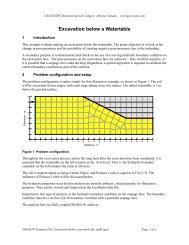
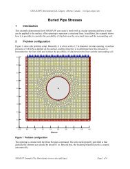
Figure 2-16 shows a stratigraphic cross section (National Research Council Report 1990). A suitable<br />
numerical model for simulating the flow regime between the groundwater divides is something like the<br />
one shown in Figure 2-17. The stratigraphic boundaries are considerably simplified for the finite element<br />
analysis.<br />
As a general rule, a model should be designed to answer specific questions. You need to constantly ask<br />
yourself while designing a model, if this feature will significantly affects the results. If you have doubts,<br />
you should not include it in the model, at least not in the early stages of analysis. Always start <strong>with</strong> the<br />
simplest model.<br />
Page 16
<strong>SEEP</strong>/W<br />
Chapter 2: Numerical <strong>Modeling</strong><br />
Figure 2-16 Example of a stratigraphic cross section<br />
(from National Research Report 1990)<br />
Figure 2-17 Finite element model of stratigraphic section<br />
The tendency of novice modelers is to make the geometry too complex. The thinking is that everything<br />
needs to be included to get the best answer possible. In numerical modeling this is not always true.<br />
Increased complexity does not always lead to a better and more accurate solution. Geometric details can,<br />
for example, even create numerical difficulties that can mask the real solution.<br />
Start simple<br />
One of the most common mistakes in numerical modeling is to start <strong>with</strong> a model that is too complex.<br />
When a model is too complex, it is very difficult to judge and interpret the results. Often the result may<br />
look totally unreasonable. Then the next question asked is - what is causing the problem? Is it the<br />
geometry, is it the material properties, is it the boundary conditions, or is it the time step size or<br />
something else? The only way to resolve the issue is to make the model simpler and simpler until the<br />
difficulty can be isolated. This happens on almost all projects. It is much more efficient to start simple and<br />
build complexity into the model in stages, than to start complex, then take the model apart and have to<br />
rebuild it back up again.<br />
A good start may be to take a homogeneous section and then add geometric complexity in stages. For the<br />
homogeneous section it is likely easier to judge the validity of the results. This allows you to gain<br />
confidence in the boundary conditions and material properties specified. Once you have reached a point<br />
where the results make sense, you can add different materials and increase the complexity of your<br />
geometry.<br />
Another approach may be to start <strong>with</strong> a steady-state analysis even though you are ultimately interested in<br />
a transient process. A steady-state analysis gives you an idea as to where the transient analysis should end<br />
up: to define the end point. Using this approach you can then answer the question of how does the process<br />
migrate <strong>with</strong> time until a steady-state system has been achieved.<br />
Page 17
Chapter 2: Numerical <strong>Modeling</strong><br />
<strong>SEEP</strong>/W<br />
It is unrealistic to dump all your information into a numerical model at the start of an analysis project and<br />
magically obtain beautiful, logical and reasonable solutions. It is vitally important to not start <strong>with</strong> this<br />
expectation. You will likely have a very unhappy modeling experience if you follow this approach.<br />
Do numerical experiments<br />
Interpreting the results of numerical models sometimes requires doing numerical experiments. This is<br />
particularly true if you are uncertain as to whether the results are reasonable. This approach also helps<br />
<strong>with</strong> understanding and learning how a particular feature operates. The idea is to set up a simple problem<br />
for which you can create a hand calculated solution.<br />
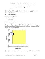
Consider the following example. You are uncertain about the results from a flux section or the meaning of<br />
a computed boundary flux. To help satisfy this lack of understanding, you could do a numerical<br />
experiment on a simple 1D case as shown in Figure 2-18. The total head difference is 1 m and the<br />
conductivity is 1 m/day. The gradient under steady state conditions is the head difference divided by the<br />
length, making the gradient 0.1. The resulting total flow through the system is the cross sectional area<br />
times the gradient which should be 0.3 m 3 /day. The flux section that goes through the entire section<br />
confirms this result. There are flux sections through Elements 16 and 18. The flow through each element<br />
is 0.1 m 3 /day, which is correct since each element represents one-third of the area.<br />
Another way to check the computed results is to look at the node information. When a head is specified,<br />
<strong>SEEP</strong>/W computes the corresponding nodal flux. In <strong>SEEP</strong>/W these are referred to as boundary flux<br />
values. The computed boundary nodal flux for the same experiment shown in Figure 2-18 on the left at<br />
the top and bottom nodes is 0.05. For the two intermediate nodes, the nodal boundary flux is 0.1 per node.<br />
The total is 0.3, the same as computed by the flux section. Also, the quantities are positive, indicating<br />
flow into the system. The nodal boundary values on the right are the same as on the left, but negative. The<br />
negative sign means flow out of the system.<br />
3<br />
2<br />
6<br />
5<br />
9<br />
8<br />
12<br />
11<br />
15<br />
3.0000e-001<br />
14<br />
18<br />
17<br />
1.0000e-001<br />
21<br />
20<br />
24<br />
23<br />
27<br />
26<br />
30<br />
29<br />
1<br />
4<br />
7<br />
10<br />
13<br />
16<br />
19<br />
22<br />
25<br />
28<br />
1.0000e-001<br />
Figure 2-18 Horizontal flow through three element section<br />
A simple numerical experiment takes only minutes to set up and run, but can be invaluable in confirming<br />
to you how the software works and in helping you interpret the results. There are many benefits: the most<br />
obvious is that it demonstrates the software is functioning properly. You can also see the difference<br />
between a flux section that goes through the entire problem versus a flux section that goes through a<br />
single element. You can see how the boundary nodal fluxes are related to the flux sections. It verifies for<br />
you the meaning of the sign on the boundary nodal fluxes. Fully understanding and comprehending the<br />
results of a simple example like this greatly helps increase your confidence in the interpretation of results<br />
from more complex problems.<br />
Page 18
<strong>SEEP</strong>/W<br />
Chapter 2: Numerical <strong>Modeling</strong><br />
Conducting simple numerical experiments is a useful exercise for both novice and experienced modelers.<br />
For novice modelers it is an effective way to understand fundamental principles, learn how the software<br />
functions, and gain confidence in interpreting results. For the experienced modeler it is an effective means<br />
of refreshing and confirming ideas. It is sometimes faster and more effective than trying to find<br />
appropriate documentation and then having to rely on the documentation. At the very least it may enhance<br />
and clarify the intent of the documentation.<br />
Model only essential components<br />
One of the powerful and attractive features of numerical modeling is the ability to simplify the geometry<br />
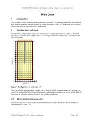
and not to have to include the entire physical structure in the model. A very common problem is the<br />
seepage flow under a concrete structure <strong>with</strong> a cut-off as shown in Figure 2-19. To analyze the seepage<br />
through the foundation it is not necessary to include the dam itself or the cut-off as these features are<br />
constructed of concrete and assumed impermeable.<br />
Figure 2-19 Simple flow beneath a cutoff<br />
Another common example is the downstream toe-drain or horizontal under drain in an embankment<br />
(Figure 2-20). The drain is so permeable relative to the embankment material that the drain does not<br />
contribute to the dissipation of the head (potential energy) loss through the structure. Physically, the drain<br />
needs to exist in the embankment, but it does not need to be present in a numerical model. If the drain<br />
becomes clogged <strong>with</strong> fines so that it begins to impede the seepage flow, then the situation is different<br />
and the drain would need to be included in the numerical model. With any material, the need to include it<br />
in the analysis should be decided in the context of whether it contributes to the head loss.<br />
Another example is the downstream shell of a zoned dam as illustrated in Figure 2-21. Often the core is<br />
constructed of fine-grained soil while the shells are highly permeable coarse granular material. If there is<br />
a significant difference between core and shell conductivities then seepage that flows through the core<br />
will drip along the downstream side of the core (usually in granular transition zones) down to an under<br />
drain. If this is the case, the downstream shell does not need to be included in the seepage analysis, since<br />
the shell is not physically involved in the dissipation of the head loss. Once again the shell needs to exist<br />
physically, but does not need to be included in the numerical seepage model.<br />
Page 19
35<br />
30<br />
20<br />
15<br />
10<br />
Chapter 2: Numerical <strong>Modeling</strong><br />
<strong>SEEP</strong>/W<br />
40<br />
25<br />
5<br />
Figure 2-20 Flow through a dam <strong>with</strong> coarse toe drain<br />
Figure 2-21 Head loss through dam core <strong>with</strong> downstream shell<br />
Including unnecessary features and trying to model adjacent materials <strong>with</strong> extreme contrasts in material<br />
properties create numerical difficulties. The conductivity difference between the core and shell of a dam<br />
may be many, many orders of magnitude. The situation may be further complicated if unsaturated flow is<br />
present and the conductivity function is very steep, making the solution highly non-linear. In this type of<br />
situation it can be extremely difficult if not impossible to obtain a good solution <strong>with</strong> the current<br />
technology.<br />
The numerical difficulties can be eased by eliminating non-essential segments from the numerical model.<br />
If the primary interest is the seepage through the core, then why include the downstream shell and<br />
complicate the analysis? Omitting non-essential features from the analysis is a very useful technique,<br />
particularly during the early stages of an analysis. During the early stages, you are simply trying to gain<br />
an understanding of the flow regime and trying to decide what is important and what is not important.<br />
While deliberately leaving components out of the analysis may at first seem like a rather strange concept,<br />
it is a very important concept to accept if you want to be an effective numerical modeler.<br />
Start <strong>with</strong> estimated material properties<br />
In the early stages of a numerical modeling project it is often good practice to start <strong>with</strong> estimates of<br />
material properties. Simple estimates of material properties and simple property functions are more than<br />
adequate for gaining an understanding of the flow regime for checking that the model has been set up<br />
properly or to verify that the boundary conditions have been properly defined. Estimated properties are<br />
usually more than adequate for determining the importance of the various properties for the situation<br />
being modeled.<br />
The temptation exists when you have laboratory data in hand that the data needs to be used in its entirety<br />
and cannot be manipulated in any way. There seems to be an inflexible view of laboratory data which can<br />
sometimes create difficulties when using the data in a numerical model. A common statement is; “I<br />
measured it in the lab and I have full confidence in my numbers”. There can be a large reality gap that<br />
exists between laboratory determined results and actual insitu soil behavior. Some of the limitations arise<br />
because of how the material was collected, how it was sampled and ultimately quantified in the lab. Was<br />
Page 20
<strong>SEEP</strong>/W<br />
Chapter 2: Numerical <strong>Modeling</strong><br />
the sample collected by the shovelful, by collecting cuttings or by utilizing a core sampler? What was the<br />
size and number of samples collected and can they be considered representative of the entire profile? Was<br />
the sample oven-dried, sieved and then slurried prior to the test being performed? Were the large particles<br />
removed so the sample could be trimmed into the measuring device? Some of these common laboratory<br />
techniques can result in unrealistic property functions. Perhaps the amount of data collected in the<br />
laboratory is more than is actually required in the model. Because money has been spent collecting and<br />
measuring the data, it makes modelers reticent to experiment <strong>with</strong> making changes to the data to see what<br />
effect it has on the analysis.<br />
It is good modeling practice to first obtain understandable and reasonable solutions using estimate<br />
material properties and then later refine the analysis once you know what the critical properties are going<br />
to be. It can even be more cost effective to determine ahead of time what material properties control the<br />
analysis and decide where it is appropriate to spend money obtaining laboratory data.<br />
Interrogate the results<br />
Powerful numerical models such as <strong>SEEP</strong>/W need very careful guidance from the user. It is easy to<br />
inadvertently and unintentionally specify inappropriate boundary conditions or incorrect material<br />
properties. Consequently, it is vitally important to conduct spot checks on the results to ensure the<br />
constraints and material properties are consistent <strong>with</strong> what you intended to define and the results make<br />
sense. It is important to check, for example that the boundary condition that appears in the results is the<br />
same as what you thought was specified defining the model. Is the intended property function being<br />
applied to the correct soil? Or, are the initial conditions as you assumed?<br />
<strong>SEEP</strong>/W has many tools to inspect or interrogate the results. You can view node or element details and<br />
there are a wide range of parameters that can be graphed for the purpose of spot checking the results.<br />
Inspecting and spot checking your results is an important and vital component in numerical modeling. It<br />
greatly helps to increase your confidence in a solution that is understandable and definable.<br />
Evaluate results in the context of expected results<br />
The fundamental question that should be asked during modeling is; “Do the results conform to the initial<br />
mental picture?” If they do not, then your mental picture needs to be fixed, there is something wrong <strong>with</strong><br />
the model or both the model and your concept of the problem need to be adjusted until they agree. The<br />
numerical modeling process needs to be repeated over and over until the solution makes perfect sense and<br />
you are able to look at the results and feel confident that you understand the processes involved.<br />
Remember the real world<br />
While doing numerical modeling it is important to occasionally ask yourself how much you really know<br />
about the input compared to the complexity of the analysis. The following cartoon portrays an extreme<br />
situation, but underscores a problem that exists when uneducated or inexperienced users try to use<br />
powerful software tools.<br />
Page 21
Chapter 2: Numerical <strong>Modeling</strong><br />
<strong>SEEP</strong>/W<br />
“If we can incorporate boundary<br />
elements rather than simple finite<br />
elephants, enhance the statistical<br />
evaluation of parameter generation<br />
and stick <strong>with</strong> the fuzzy sets, I am<br />
confident that accuracy will be<br />
increased to at least the fourth<br />
decimal place.”<br />
“Put another shovel<br />
full in Pat! It is fullcores<br />
they’re wanting!”<br />
Note: origins of this figure are unknown at time of printing.<br />
2.6 How not to model<br />
As mentioned earlier in this chapter, it is completely unrealistic to expect to set up a complex model at the<br />
start of a project and immediately obtain realistic, understandable and meaningful results. There are far<br />
too many parameters and issues which can influence the results, so if this is your expectation, then<br />
modeling is going to lead to major disappointments.<br />
For novice modelers; the initial reaction when faced <strong>with</strong> incomprehensible results is that something must<br />
be wrong <strong>with</strong> the software. It must be a limitation of the software that the solution is inappropriate or<br />
completely senseless. It is important to remember that the software is very powerful; it can keep track of<br />
millions of pieces of information and do repetitive computations which are far beyond the capability of<br />
the human mind. Without the software it would not be possible to make these types of analyses. The<br />
software by itself is extremely powerful numerically speaking, but essentially unintelligent. Conversely,<br />
the human mind has the capability of logic and reasoning, but has significant limitations retaining large<br />
amounts of digital data. It is the combination of the human mind together <strong>with</strong> the capability of a<br />
computer that makes numerical modeling so immensely powerful. Neither can do the task in isolation.<br />
The software can only be used effectively under the careful guidance and direction of the modeler.<br />
Sometimes it is suggested that due to a time limitation, it is not possible to start simple and then progress<br />
slowly to a more complex analysis. A solution is needed quickly and since the budget is limited, it is<br />
necessary to immediately start <strong>with</strong> the ultimate simulation. This approach is seldom, if ever, successful.<br />
Usually this leads to a lot of frustration and the need to retreat to a simpler model until the solution is<br />
understandable and then build it up again in stages. Not following the above “how to” modeling<br />
procedures generally leads to requiring more time and financial resources than if you follow the<br />
recommended modeling concepts.<br />
Page 22
<strong>SEEP</strong>/W<br />
Chapter 2: Numerical <strong>Modeling</strong><br />
Remember, the software is only as good as your ability to guide and direct it. The intention of this<br />
document is to assist you in providing this guidance and direction so that you can take full advantages of<br />
the power the software can offer.<br />
2.7 Closing remarks<br />
As noted in the introduction, numerical modeling is a relatively new area of practice. Most university<br />
educational curricula do not include courses on how to approach numerical modeling and, consequently,<br />
the skill is often self-taught. As software tools such as <strong>SEEP</strong>/W become increasingly available at<br />
educational institutions and educators become comfortable <strong>with</strong> these types of tools, classes and<br />
instruction should improve <strong>with</strong> respect to numerical modeling.<br />
When the numerical analysis software tool, <strong>SEEP</strong>/W <strong>2007</strong>, is effectively utilized as it was intended to be<br />
used, it becomes an immensely powerful tool, making it possible to do highly complex analyses. It can<br />
even lead to new understandings about actual physical process.<br />
The process of modeling is a journey of discovery, a way of learning something new about the complex<br />
behavior of our physical world. It is a process that can help us understand highly complex, real physical<br />
process so that we can exercise our engineering judgment <strong>with</strong> increased confidence.<br />
Page 23
Chapter 2: Numerical <strong>Modeling</strong><br />
<strong>SEEP</strong>/W<br />
Page 24
<strong>SEEP</strong>/W<br />
Chapter 3: Geometry and Meshing<br />
3 Geometry and Meshing<br />
3.1 Introduction<br />
Finite element numerical methods are based on the concept of subdividing a continuum into small pieces,<br />
describing the behavior or actions of the individual pieces and then reconnecting all the pieces to<br />
represent the behavior of the continuum as a whole. This process of subdividing the continuum into<br />
smaller pieces is known as discretization or meshing. The pieces are known as finite elements.<br />
In <strong>GeoStudio</strong>, the geometry of a model is defined in its entirety prior to consideration of the discretization<br />
or meshing. This is an approach that is new in <strong>GeoStudio</strong> <strong>2007</strong>. Furthermore, automatic mesh<br />
generation algorithms have now advanced sufficiently to enable a well behaved, numerically robust<br />
default discretization often <strong>with</strong> no additional effort required by the user. Of course, it is still wise to<br />
view the default generated mesh but any required changes can easily be made by changing a single global<br />
element size parameter, by changing the number of mesh divisions along a geometry line object, or by<br />
setting a required mesh element edge size.<br />
Figure 3-1 shows the fully defined model for a soil excavation project. The entire model was built using<br />
various geometry items.<br />
• Soil regions were specified;<br />
• Geometry lines were drawn at the locations of tie-back anchors and cutoff wall;<br />
• Soil material models were created and assigned onto the geometry objects and<br />
• Pre-defined boundary conditions were drawn on the region edges.<br />
As a final step before solving, the mesh properties were viewed and adjustments made. In this case, the<br />
global element size was specified as 1.0 meter. In addition, the geometry line representing the grouted<br />
section of the anchors was discretized. The pre-stressed length of the anchors was intentionally left nondiscretized.<br />
The final model is shown in Figure 3-2.<br />
Now that you have a basic introduction to the concept of building your model using geometry objects, we<br />
can discuss each type of object in more detail. We must also have a discussion about the finite elements<br />
themselves, as these are the backbone to the entire finite element method.<br />
Page 25
Chapter 3: Geometry and Meshing<br />
<strong>SEEP</strong>/W<br />
20<br />
18<br />
16<br />
14<br />
Elevation - m<br />
12<br />
10<br />
8<br />
6<br />
4<br />
2<br />
0<br />
0 5 10 15 20 25 30 35 40 45<br />
Distance - m<br />
Figure 3-1 Fully defined geometry for soil excavation model<br />
20<br />
18<br />
16<br />
14<br />
Elevation - m<br />
12<br />
10<br />
8<br />
6<br />
4<br />
2<br />
0<br />
0 5 10 15 20 25 30 35 40 45<br />
Distance - m<br />
Figure 3-2 Default element discretization for model using 1m global element size<br />
constraint<br />
3.2 Geometry objects in <strong>GeoStudio</strong><br />
New to <strong>GeoStudio</strong> in <strong>2007</strong> is the concept that the entire model is defined as a series of geometry objects.<br />
These objects can be soil regions, circular openings line objects, surface regions, and point objects. These<br />
objects are shown in the images below – as defined and then <strong>with</strong> the mesh applied.<br />
Page 26
<strong>SEEP</strong>/W<br />
Chapter 3: Geometry and Meshing<br />
Free line in space<br />
Surface layers<br />
Region points<br />
Circular region<br />
Free line<br />
Soil region<br />
Free point<br />
Region lines<br />
Figure 3-3 Available geometry objects<br />
Figure 3-4 Mesh pattern for example model<br />
Each of these geometry objects can have additional objects assigned to them such as material or boundary<br />
conditions objects. They can also have special properties, such as mesh element type, size and integration<br />
order.<br />
Let us consider each in turn.<br />
Soil regions, points and lines<br />
<strong>GeoStudio</strong> uses the concept of regions and points to define the geometry of a problem and to facilitate<br />
discretization of the problem. The attraction of using regions is that they replicate what we intuitively do<br />
as engineers and scientists to illustrate concepts and draw components of a system. To draw a<br />
stratigraphic section, for example, we intuitively draw the different soil types as individual regions.<br />
The use of regions offers all the advantages of dividing a large domain into smaller pieces, working and<br />
analyzing the smaller pieces, and then connecting the smaller pieces together to obtain the behavior of the<br />
whole domain, exactly like the concept of finite elements. Generally, all physical systems have to be<br />
broken down into pieces to create, manage and control the whole body.<br />
A collection of highly adaptive individual pieces that can be joined together makes it possible to describe<br />
and define almost any complex domain or physical system. Such an approach is more powerful and can<br />
Page 27
Chapter 3: Geometry and Meshing<br />
<strong>SEEP</strong>/W<br />
be applied to a wider range of problems than any system that attempts to describe the whole domain as a<br />
single object.<br />
Regions may be simple straight-sided shapes like quadrilaterals or triangles or a free form, multi-sided<br />
polygon. Figure 3-5 illustrates a domain constructed using one quadrilateral and two triangular regions.<br />
Also shown in this figure are the region points and the region lines. Each segment of a region edge<br />
between any two adjacent points is called a line. Both points and lines can have special properties as<br />
discussed in the next sections. In this figure the lines and points are not “free” as they belong to a region.<br />
They do, however have similar behavior to free points and lines.<br />
Figure 3-6 shows a multi-sided polygonal region defined using 10 points. There is no restriction on the<br />
number of points in a region. However, the rule of thumb to keep things simple is always encouraged.<br />
Points<br />
Lines<br />
Figure 3-5 Illustration of a region’s lines and points<br />
10<br />
9<br />
8<br />
7<br />
6<br />
5<br />
4<br />
3<br />
1 2<br />
Figure 3-6 A multi-side polygonal region<br />
Points can be selected and moved to modify the shape and position of regions, which provides for great<br />
flexibility in making adjustments and alterations to a problem definition.<br />
Page 28
<strong>SEEP</strong>/W<br />
Chapter 3: Geometry and Meshing<br />
15 16<br />
14<br />
17<br />
13<br />
11 12<br />
Figure 3-7 Regions of different size<br />
Points are also required in order to join regions of different sizes and to control the meshing for specific<br />
purposes. Figure 3-7 shows a homogeneous soil region <strong>with</strong> a concrete footing region. The foundation<br />
region is made up of Points 11, 12, 13, 17 and 14. The footing region is made up of Points 14, 17, 16, and<br />
15. Points 14 and 17 are common to both regions and therefore the two regions are properly joined and<br />
connected along this edge. In addition, Point 17 ensures that an element node will be created and will<br />
exist at the edge of the footing, which is required for proper meshing. It also breaks up the region edge<br />
between points 13 and 14 so that a unique boundary condition may be placed along the edge sub-section.<br />
When a region is defined, it is restricted to having:<br />
One type of material,<br />
One type of element meshing pattern (or no mesh),<br />
One order of elements; either first- or second-order, and<br />
One integration order.<br />
More information on finite elements is provided later in this chapter.<br />
Free points<br />
As seen in the illustrations above, regions are made up of a series of points. It is also possible for a point<br />
to exist <strong>with</strong>in a region or outside of a region on its own. By default, a finite element “node” must exist at<br />
the location of all points, whether region corner points or free points. The advantage of this is that by<br />
placing a “free point” you can ensure that a boundary condition is applied at the desired location.<br />
In past <strong>version</strong>s of GEO-SLOPE software, all boundary conditions were applied directly to mesh nodes or<br />
mesh element edges. This is no longer the approach to use. Now, all boundary conditions must be<br />
applied directly to region lines, region (or free) points or geometry lines. The power in this new approach<br />
will be readily evident to the user who decides to change the default generated mesh. In the past,<br />
changing the mesh required that all boundary conditions and soil properties (in some cases) were lost or<br />
attempted to be re-applied. Now, because properties and boundary condition exist as objects on geometry<br />
items, the mesh can be changed <strong>with</strong> no threat of having to re-do parts of the model set up.<br />
Free lines<br />
A free line is a line object that does not make up any part of a region edge. They can be very useful for<br />
applying anchors to a model or for specifying a geo-fabric or insulation layer. They can also be used for<br />
creating structural components that are partially in the soil and partially outside the soil. Here are some<br />
examples…<br />
Page 29
Chapter 3: Geometry and Meshing<br />
<strong>SEEP</strong>/W<br />
50<br />
37 38<br />
23 24 25<br />
Figure 3-8 Truss loading model<br />
In Figure 3-8 structural bar properties have been applied to a pattern of free lines in order to determine<br />
displacements under loading for the truss system.<br />
4<br />
18<br />
5<br />
17<br />
Figure 3-9 Anchors on lines (line is partially meshed)<br />
Figure 3-9 shows two key aspects of free lines. A free line in two segments has been drawn to model a tie<br />
back anchor. The upper length of the free line was left un-discretized (i.e., independent of the finite<br />
element mesh) while the lower length is incorporated into the mesh. The lower end represents a beam<br />
structural member which requires that it is aligned <strong>with</strong> the surrounding soil elements. The upper length<br />
represents a structural bar element which only acts in tension or compression and only has an active force<br />
and stiffness at its end points which do coincide <strong>with</strong> nodal locations. It does not interact <strong>with</strong> the soil so<br />
does not need to share a mesh <strong>with</strong> the soil except at its end points.<br />
Page 30
<strong>SEEP</strong>/W<br />
Chapter 3: Geometry and Meshing<br />
Figure 3-10 Lines <strong>with</strong> material model “none” (no flow) assigned to simulate lysimeter<br />
collection basin in waste beneath an engineered soil cover<br />
Figure 3-10 shows the use of free lines to construct a lysimeter collection basin beneath an engineered<br />
soil cover system. The line was assigned a material model of “none” to simulate a no flow condition (i.e.,<br />
a null material). This is a key point to understand, that the line was assigned a material model. When this<br />
is done, the line inherits the behavioral properties of the material assigned and a special interface element<br />
is added to the line mesh. The interface behavior depends on the application being solved. In this<br />
example, the interface has “no flow” across it. In a stress-deformation model, the interface on the line<br />
may be assigned soil – structure friction/slippage properties. Interface elements are discussed in more<br />
detail in the next section.<br />
Interface elements on lines<br />
In the previous section the concept of applying a material model to a single line was introduced. The<br />
actual material models that can be used are dependent on the analysis being solved. For example, in<br />
<strong>SEEP</strong>/W an interface model may be used to represent a geo-fabric or a null material to represent a barrier<br />
to flow. In TEMP/W it may be a thin insulation layer. In SIGMA/W, the material model may describe<br />
the friction properties between soils, or a soil and a structure such as a cutoff wall. You can read about all<br />
of these models in the respective engineering books.<br />
Interface material on lines<br />
Figure 3-11 Illustration of "interface elements" on geometry lines<br />
Page 31
Chapter 3: Geometry and Meshing<br />
<strong>SEEP</strong>/W<br />
The discussion now will focus on how to apply an interface region to a line object. There are two ways to<br />
do this. There is a Draw Line Material Properties command in which you can choose a material model<br />
you have defined and apply it to a line by clicking just next to a line as shown in Figure 3-12. You can<br />
assign a different property to either side of a line. If you use this option, you are specifying the material<br />
as well as creating special thin “interface” elements. You can then go back and change the element<br />
thickness from its default value using the Draw Mesh Properties command and choosing the line.<br />
Figure 3-12 Using the Draw Line Material command to assign an interface model to a line<br />
The second option for specifying an interface model on a line is to first create the thin elements and then<br />
assign the material to the line. You can use the Draw Mesh Properties command, select the line, choose<br />
the Generate Interface Elements option and specify an interface element thickness. This process is<br />
illustrated in Figure 3-13.<br />
The actual thickness of the interface elements may or may not have physical meaning but the material<br />
model assigned to them will hold some meaning. If, for example, the interface represents an insulation<br />
layer in TEMP/W, then the thickness is relevant. However, if the interface describes the frictional<br />
behavior between two sliding blocks, then the thickness specified is not factored in the solution and it can<br />
be specified only to satisfy your presentation needs.<br />
Page 32
<strong>SEEP</strong>/W<br />
Chapter 3: Geometry and Meshing<br />
Figure 3-13 Using Draw Mesh Properties to create interface elements on selected line<br />
Circular openings<br />
A circular opening is a type of region that “floats” over top of another soil region. It is created using a<br />
Draw command and is defined by its center point and one point on its circumference. The region can be<br />
dragged to a different location or its circumference point can be moved to change the size of the opening.<br />
Like all other regions, it can have a mesh assigned to it; it can have material properties assigned to its<br />
edge (such as a tunnel liner interface material); and it can have boundary conditions assigned to its edge<br />
or center point.<br />
Figure 3-14 shows a circular opening region that was placed on top of an existing soil region. The<br />
circular region was applied by clicking on the desired center point and then dragging the radius point to a<br />
desired location. Once defined, the region can be designated to be a mesh opening or an un-meshed<br />
opening or hole. A mesh may be necessary to obtain in-situ stresses prior to excavation. A hole may be<br />
necessary to simulate a pipe or culvert. In the opening presented in the figure, interface elements have<br />
been added to the tunnel face. This will make it possible to apply a structural beam to the face <strong>with</strong> a<br />
soil-structure interaction model applied between the beam and soil.<br />
Page 33
Chapter 3: Geometry and Meshing<br />
<strong>SEEP</strong>/W<br />
Figure 3-14 Circular region <strong>with</strong> defined center point, radius point and interface elements<br />
3.3 Mesh generation<br />
In <strong>GeoStudio</strong> all meshing is now fully automatic. There is no longer the ability to draw individual “finite<br />
elements.” In addition, there is no worry whether the mesh will be compatible across different regions or<br />
whether your material properties or boundary conditions will disappear if you change the mesh.<br />
When a geometry region or line is initially drawn it is by default un-meshed. A default mesh is generated<br />
for the soil regions when you first use the Draw Mesh Properties command, which you may accept or<br />
modify. You may alter the size of the elements at a global level for the entire mesh, <strong>with</strong>in any one or<br />
more regions, or along a line or around a point. You may specify mesh density as a real length unit, as a<br />
ratio of the global mesh size, or as the number of divisions along a line edge. Generally, however, it is<br />
recommended that you limit altering the mesh to changing the global density and then, if necessary, at a<br />
few limited locations where finer or coarser density is needed.<br />
Meshing options and available patterns are shown in the image below.<br />
Figure 3-15 Draw Mesh Properties options<br />
Page 34
<strong>SEEP</strong>/W<br />
Chapter 3: Geometry and Meshing<br />
Structured mesh<br />
Figure 3-16 presents what is known as a structured mesh because the elements are ordered in a consistent<br />
pattern and are of only two shapes and sizes. A structured mesh for a non-symmetrical geometry shape<br />
requires that several soil regions are created and the meshing is controlled <strong>with</strong>in each region. This is<br />
likely more work to accomplish and will not yield a significant improvement in results. More efficient,<br />
automatic meshing options <strong>with</strong> good numerical performance are available and will be discussed in the<br />
next section. A structured mesh is created using either a rectangular grid of quads or a triangular grid of<br />
quads/triangles.<br />
Unstructured quad and triangle mesh<br />
The fully structured mesh shown in Figure 3-16 may require several regions to be defined so that you can<br />
control the meshing at a detailed level in order to maintain structure. A new meshing pattern is available<br />
that will automatically generate a well behaved unstructured pattern of quadrilateral and triangular<br />
elements as shown in Figure 3-17. In our opinion, this mesh option should be the first one you choose as<br />
it will meet your needs in most cases.<br />
9<br />
1<br />
8<br />
2 3<br />
7<br />
10<br />
4 5 6<br />
32 33<br />
Figure 3-16 Structured mesh<br />
34 35<br />
31<br />
36<br />
Unstructured triangular mesh<br />
Figure 3-17 Mixed quad and triangle unstructured mesh<br />
The diagram in Figure 3-18 shows the same section as in Figure 3-16, but this time <strong>with</strong> an unstructured<br />
triangular mesh. In this case the mesh is automatically created using Delaunay triangulation techniques.<br />
One of the great attractions of unstructured meshing is that almost any odd-shaped region can be meshed.<br />
Page 35
Chapter 3: Geometry and Meshing<br />
<strong>SEEP</strong>/W<br />
This meshing simplicity however has some numerical and interpretation consequences as discussed in<br />
more detail in the Structured versus Unstructured Section below.<br />
32 33<br />
34 35<br />
31<br />
36<br />
Figure 3-18 Unstructured triangular mesh<br />
Triangular grid regions<br />
<strong>GeoStudio</strong> has a special structured pattern for triangular regions called a triangular grid of<br />
quads/triangles. The next figure (Figure 3-19) shows a typical triangular region <strong>with</strong> the resulting<br />
structured mesh. The elements are a mixture of squares, rectangles, trapezoids and triangles. The use of<br />
this pattern is fairly general, but it does have some limitations and restrictions.<br />
3<br />
1 2<br />
Figure 3-19 Triangular grid region<br />
It is useful to think of the region as having three sides: a short side, an intermediate length side and a long<br />
side. The algorithm attempts to sort the edges so that the sides go from the shortest to the longest in a<br />
counter-clockwise direction. In this example, the shortest side is 3-1, the intermediate 1-2 and the longest<br />
2-3.<br />
The meshing algorithm works best when the number of divisions is controlled on the shortest and<br />
intermediate sides. To retain the even pattern shown in Figure 3-19, the number of divisions should be<br />
defined on the shortest side first and then on the intermediate side. The number of divisions on the<br />
intermediate side can be an even multiple of the number on the shortest side. In the above example, the<br />
shortest side has 5 divisions and the intermediate side can have 10, or 2 times that of the shortest side.<br />
The algorithm works best and gives the best structured mesh if the numbers of divisions on the longest<br />
side are left undefined allowing the algorithm to compute the appropriate number of divisions.<br />
If a triangular region is mixed in <strong>with</strong> other more general regions, <strong>GeoStudio</strong> will attempt to ensure mesh<br />
compatibility. Sometimes however it may not be possible to adhere to the requirements for generating a<br />
structured mesh in a triangular region and then <strong>GeoStudio</strong> will substitute an unstructured mesh.<br />
Page 36
<strong>SEEP</strong>/W<br />
Chapter 3: Geometry and Meshing<br />
Rectangular grid of quads<br />
Figure 3-20 shows the same region geometry meshed <strong>with</strong> the rectangular grid of quads pattern. This is a<br />
structured mesh but has the potential to be more difficult to control. The mesh pattern on the left side is<br />
very nice but near the base of the slope the quad shape is starting to distort. This distortion could be<br />
controlled by adding more region points along the bottom edge but this will still result in a mesh <strong>with</strong><br />
large elements on the left and thinner elements on the right. This mesh pattern is ideally suited for four<br />
sided regions only.<br />
32 33<br />
34 35<br />
31<br />
36<br />
Figure 3-20 Rectangular grid of quad elements<br />
3.4 Surface layers<br />
At the ground surface conditions change in response to the climate and climatic conditions can change<br />
dramatically over short periods of time. For example, the ground maybe highly desiccated near the<br />
surface on a hot day before a thunderstorm. In a short period of time, the soil changes from being very dry<br />
to being saturated. Another example may be penetration of frost from the ground surface. To numerically<br />
deal <strong>with</strong> rapid and dramatic boundary changes it is necessary to have fine discretization near the ground<br />
surface. <strong>GeoStudio</strong> has a special procedure for constructing a surface layer that can be finely discretized.<br />
Figure 3-21 illustrates a surface layer placed over the surface of a larger region. The surface layer<br />
capability is also invaluable for discretizing features such as engineered soil covers over waste material,<br />
which may consist of several relatively thin layers of soil which also require fine discretization.<br />
The ability to construct a surface layer is available in VADOSE/W, <strong>SEEP</strong>/W and TEMP/W. In <strong>SEEP</strong>/W<br />
the surface layer is used to tell the solver that it should track seepage face flows and infiltration events for<br />
any unit flux boundary condition. As a result, water that does not immediately infiltrate the ground is not<br />
considered lost from the analysis, but is allowed to pond and build up a positive pressure head in any<br />
user-defined low points along the surface. The other <strong>GeoStudio</strong> modules cannot be used to construct a<br />
surface layer, but once the surface mesh has been created it will exist in all the other modules.<br />
Consequently, if a layer has been created for a <strong>SEEP</strong>/W analysis, the surface layer will also be part of a<br />
SLOPE/W analysis, since <strong>GeoStudio</strong> uses only one geometry definition <strong>with</strong>in a single data file.<br />
Once the main soil profile has been meshed, a special Draw Surface Layer command can be used to build<br />
up a single or multi layer region along all or part of a ground surface. Parameters such as the soil type and<br />
individual layer geometry are defined and a quadrilateral element mesh <strong>with</strong> vertically oriented nodes is<br />
automatically built on top of the existing ground region. The structure of the mesh will ensure optimum<br />
numerical stability during the solution.<br />
Quadrilateral elements are much better for modeling ground surface processes because the primary<br />
unknown gradients are usually steeper in a direction perpendicular to the surface. The presence of<br />
triangular elements in thin layers near the surface causes excessive fluctuation in the computed results<br />
Page 37
Chapter 3: Geometry and Meshing<br />
<strong>SEEP</strong>/W<br />
relative to the orientation of the triangular elements. Also, dealing <strong>with</strong> plant root zones in the<br />
VADOSE/W model necessitates that element nodes in the surface layer all fall on vertical lines.<br />
Moreover, using quadrilaterals greatly reduces the number of elements required, an important<br />
consideration when dealing <strong>with</strong> situations that will be very computationally intensive.<br />
Figure 3-21 Illustration of a surface layer mesh<br />
Surface layers have special viewing options. Consider the two meshes illustrated in Figure 3-22. The left<br />
diagram shows a surface layer <strong>with</strong>out all the cluttering details as illustrated on the right. When many thin<br />
elements are located in a close proximity to each other, they can appear indistinguishable when viewed<br />
from a far away scale. By optionally turning off the surface mesh details a clearer image of the structure<br />
of the near surface soil layers can be viewed.<br />
Figure 3-23 is another illustration of this optional viewing concept. The left diagram in the figure shows<br />
the detailed mesh and soil layers across the 0.75m thick surface region and the right diagram leaves the<br />
details out, but still shows the layer colors. A couple of additional key points can be made in regards to<br />
the figure. Notice that bottom two elements of the left diagram are the same soil type as the main<br />
underlying soil. This is a good mesh design strategy – that being to have the bottom most layer of the<br />
surface mesh be made of the same soil as the existing ground. Consider if the bottom layer of the surface<br />
soil was VERY different from the underlying soil. If a finely spaced mesh was placed directly on top of<br />
the different underlying soil then the numerical integration of material properties at the common mesh<br />
node between the two soils would be less accurate because of the influence of the large element area from<br />
the material below the common nodal point. By having the bottom layer of the surface layer be the same<br />
as the underlying soil, the element shapes are very similar in size and aspect at the common nodal point<br />
between the two very contrasting soils.<br />
The second point to node from Figure 3-23 is that in the right diagram the nodes that are located at the<br />
interface between two soils are still viewable even though the main mesh details are not. This is<br />
intentional so that you can easily see and graph data at nodes that are used for automatic tracking of<br />
interlayer fluxes in the VADOSE/W model.<br />
Page 38
<strong>SEEP</strong>/W<br />
Chapter 3: Geometry and Meshing<br />
Figure 3-22 Surface region mesh <strong>with</strong> details off (left) and on (right)<br />
Figure 3-23 Close up of surface details on and off (note inter-layer nodes still visible in<br />
figure on right)<br />
Boundary flux modeling <strong>with</strong> rainfall infiltration, runoff, snow melt etc. can be very numerically<br />
demanding from a convergence perspective. Potential problems can be made worse if the shape of the<br />
surface mesh is not “realistic.” Consider the two meshes illustrated in Figure 3-24 and Figure 3-25. In the<br />
first figure, the ground profile has rounded corners which are much more natural and much more<br />
numerically friendly. In the second figure, changes in slope angle are represented by a sharp break. This<br />
sharp break is not only un-natural, but the shape of the individual elements right at the transition points<br />
creates numerical problems if there are large changes in boundary condition type at different nodes <strong>with</strong>in<br />
the same element. This would be the case when the corner node at the bottom of the slope becomes a<br />
seepage face point while the next node up slope is still an infiltration node. Basically, it is better to build<br />
the mesh to look somewhat natural.<br />
g<br />
Figure 3-24 Mesh showing rounded surface slope breaks<br />
Page 39
Chapter 3: Geometry and Meshing<br />
<strong>SEEP</strong>/W<br />
Figure 3-25 Mesh showing angular surface slope breaks<br />
In order to create a surface mesh <strong>with</strong> more rounded features it is necessary to build the underlying soil<br />
mesh <strong>with</strong> the same rounded profile. This is easily accomplished in <strong>GeoStudio</strong> by adding additional<br />
region points near a slope break such that the region points can be moved slightly to create a rounded<br />
profile. This is the case in Figure 3-26 below where three region points are used at both the toe and crest<br />
of the slope. Also notice that three region points are used on the bottom of the mesh beneath the toe and<br />
crest location. This is a useful tip to remember. When you want to have more control over the trans-finite<br />
element mesh you should add region points on opposite sides of the mesh from where you need the detail.<br />
As a final note, adding region points can be done at any time – even after the surface layer is created.<br />
When the region beneath a surface layer is changed, the surface layer above it will be automatically<br />
regenerated to ensure mesh compatibility <strong>with</strong> the region below.<br />
Figure 3-26 Region mesh <strong>with</strong> region corner points viewed and surface details not<br />
viewed<br />
3.5 Joining regions<br />
Compatibility must be maintained between regions to ensure the regions are connected. Regions must be<br />
joined at the region points and points must be common to adjoining regions for the regions to be properly<br />
connected. <strong>GeoStudio</strong> has a number of features to assist in achieving region compatibility.<br />
The following are some of the main characteristics:<br />
Page 40
<strong>SEEP</strong>/W<br />
Chapter 3: Geometry and Meshing<br />
If the cross-hair symbol moves close to an existing point, the symbol will snap to the existing<br />
point.<br />
A new point will be created if the cursor is on the perimeter of an existing region. The new point<br />
will then be common to the new region and to the existing region.<br />
Points in between selected points are automatically selected along an existing region edge unless<br />
the Ctrl key is held down.<br />
Consider the diagram in Figure 3-27. Region 1 is drawn first and Region 2 can be drawn by clicking on<br />
Points 7, 3, 8 and 9. Points 4, 5 and 6 are automatically added to Region 2.<br />
9<br />
8<br />
7<br />
6<br />
2<br />
5<br />
4<br />
3<br />
1<br />
1 2<br />
Figure 3-27 Regions joined along jagged line<br />
9<br />
8<br />
7<br />
2<br />
5<br />
3<br />
6<br />
4<br />
1<br />
1 2<br />
Figure 3-28 Adjoining regions <strong>with</strong> an open space<br />
Sometimes it may be desirable to create an open area in a mesh and then it is necessary to hold down the<br />
Ctrl key when going from Point 7 to 3 or 3 to 7. Doing this results in a mesh as shown in Figure 3-28. In<br />
this case the Ctrl key was held down after clicking on Point 7, but before clicking on Point 3.<br />
Additional details on joining regions are presented in the on-line help.<br />
3.6 Meshing for transient analyses<br />
<strong>Modeling</strong> transient processes requires a procedure to march forward in time increments. The time<br />
increments are referred to in <strong>GeoStudio</strong> as time steps. Selecting and controlling the time step sequence is<br />
a topic in itself and will be dealt <strong>with</strong> later. Obtaining acceptable transient solutions is not only influenced<br />
by the time steps, but also by the element size. In a contaminant transport advection-dispersion analysis<br />
(CTRAN/W) it is necessary to have a time step sufficiently large to allow an imaginary contaminant<br />
Page 41
Chapter 3: Geometry and Meshing<br />
<strong>SEEP</strong>/W<br />
particle to move a significant distance relative to the element size, while at the same time not have the<br />
time step size be so large as to allow the particle to jump across several elements. The particle should, so<br />
to speak, make at least one stop in each element. In CTRAN/W this is controlled by the Peclet and<br />
Courant criteria.<br />
In a simulation of consolidation, the time step size for the first time step needs to be sufficiently large so<br />
that the element next to the drainage face consolidates by at least 50 percent. Achieving this is related to<br />
the element size; the larger the element the greater the required initial time step. If the time step size is too<br />
small, the computed pore-water pressures may be unrealistic.<br />
The important point in this section on meshing is to realize that meshing, more particularly element sizes,<br />
comes into play in a transient analysis. Rules and guidelines for selecting appropriate time stepping are<br />
discussed elsewhere <strong>with</strong> reference to particular types of analysis.<br />
3.7 Finite elements<br />
Discretization or meshing is one of the three fundamental aspects of finite element modeling. The other<br />
two are defining material properties and boundary conditions. Discretization involves defining geometry,<br />
distance, area, and volume. It is the component that deals <strong>with</strong> the physical dimensions of the domain.<br />
A numerical book-keeping scheme is required to keep track of all the elements and to know how all the<br />
elements are interconnected. This requires an ordered numbering scheme. When finite element methods<br />
were first developed, creating the mesh numbering was very laborious. However, many computer<br />
algorithms are now available to develop the mesh and assign the element numbering. Developing these<br />
algorithms is in some respects more complex than solving the main finite element equations. <strong>GeoStudio</strong><br />
has its own system and algorithms for meshing, which are designed specifically for the analysis of<br />
geotechnical and geo-environmental problems.<br />
Some human guidance is required to develop a good finite element mesh in addition to using the powerful<br />
automatic meshing algorithms available. One of the issues, for example, is mesh size. Computers,<br />
particularly desktop or personal computers, have limited processing capability and therefore the size of<br />
the mesh needs to be limited. Variable mesh density is sometimes required to obtain a balance between<br />
computer processing time and solution requirements. Ensuring that all the elements are connected<br />
properly is another issue. Much of this can be done <strong>with</strong> the meshing algorithm, but it is necessary for the<br />
user to follow some fundamental principles. In finite element terminology this is referred to as ensuring<br />
mesh compatibility. <strong>GeoStudio</strong> ensures mesh compatibility <strong>with</strong>in a region and for the most part ensures<br />
mesh compatibility across adjacent regions, but it is still possible to create a situation whereby mesh<br />
incompatibility exists. The user needs to provide some guidance in ensuring compatibility between<br />
regions.<br />
The purpose of this chapter is to introduce some of the basic concepts inherent in meshing and outline<br />
some procedures which must be followed when developing a mesh. An understanding of these<br />
fundamentals is vital to proper discretization.<br />
Much of this chapter is devoted to describing the meshing systems and the features and capabilities<br />
available in <strong>GeoStudio</strong>. In addition, there are also discussions on the selection, behavior and use of<br />
various element types, sizes, shapes and patterns. A summary of practical guidelines for good meshing<br />
practice are also outlined.<br />
Page 42
<strong>SEEP</strong>/W<br />
Chapter 3: Geometry and Meshing<br />
3.8 Element fundamentals<br />
Element nodes<br />
One of the main features of a finite element are the nodes. Nodes exist at the corners of the elements or<br />
along the edges of the elements. Figure 3-29 and Figure 3-30 show the nodes, represented as black dots.<br />
The nodes are required and used for the following purposes:<br />
The positions of the nodes in a coordinate system are used to compute the geometric<br />
characteristics of the element – such as length, area or volume.<br />
The nodes are used to describe the distribution of the primary unknowns <strong>with</strong>in the element. In<br />
the <strong>SEEP</strong>/W formulation, the primary field variable is the hydraulic head or pore-water<br />
pressure.<br />
The nodes are used to connect or join all the elements <strong>with</strong>in a domain. All elements <strong>with</strong> a<br />
common node are connected at that node. It is the common nodes between elements that<br />
ensure compatibility, which is discussed in further detail below.<br />
All finite element equations are formed at the nodes. All elements common to a single node<br />
contribute to the characteristics and coefficients that exist in the equation at that node, but it is<br />
the equation at the node that is used to compute the primary unknown at that node. In other<br />
words, the seepage equation is developed for each node and the material properties which are<br />
used <strong>with</strong>in the equations are contributed from the surrounding elements.<br />
There can be multiple finite element equations developed at each node depending on the degrees of<br />
freedom. In seepage analysis there is only one degree of freedom at each node, which is the head or porewater<br />
pressure. The number of finite element equations to be solved is equal to the number of nodes used<br />
to define the mesh. In a 2D stress-deformation analysis, there are two degrees of freedom at each node –<br />
displacement x and displacement y. Consequently, the number of equations for the whole domain is equal<br />
to two times the number of nodes. In a coupled consolidation analysis there are three degrees of freedom<br />
at each node – displacement x, displacement y and pore-water pressure. For a coupled consolidation<br />
analysis the total number of equations required to solve the problem is three times the number of nodes.<br />
Since the number of finite element equations is related to the number of nodes, the number of nodes in a<br />
problem is one of the main factors in the computing time required to solve for the primary unknowns.<br />
Field variable distribution<br />
In a finite element formulation it is necessary to adopt a model describing the distribution of the primary<br />
variable <strong>with</strong>in the element (e.g., total head). The distribution could be linear or curved.<br />
For a linear distribution of the primary unknown, nodes are required only at the element corners. The two<br />
nodes (points) along an edge are sufficient to form a linear equation. Figure 3-29 illustrates this situation.<br />
Elements <strong>with</strong> nodes existing at the corners are referred to as first-order elements.<br />
Page 43
Chapter 3: Geometry and Meshing<br />
<strong>SEEP</strong>/W<br />
Figure 3-29 Primary field variable distribution in first-order elements<br />
The derivative of the primary unknown <strong>with</strong> respect to distance is the gradient. For a linear distribution<br />
the gradient is consequently a constant. In the context of a seepage formulation the primary unknown is<br />
the hydraulic head. The derivative of head <strong>with</strong> respect to distance is the seepage gradient and the<br />
gradient is therefore constant <strong>with</strong>in a first order element.<br />
With three nodes defined along an edge, we can write a quadratic equation describing the distribution of<br />
the primary unknown <strong>with</strong>in the element. Consequently the distribution of the primary unknown can be<br />
curved as shown in Figure 3-30. The derivative of the quadratic head distribution results in a linear<br />
gradient distribution. Elements <strong>with</strong> three or more nodes along an edge are referred to as higher order<br />
elements. More specifically, an element <strong>with</strong> three nodes along an edge is known as a second-order<br />
element.<br />
Figure 3-30 Primary field variable distribution in higher-order elements<br />
Higher order elements are more suited to problems where the primary unknowns are vectors as in a stressdeformation<br />
analysis (deformation x and y). When the primary unknown is a scalar value as in a seepage<br />
formulation, there is often little to be gained by using higher-order elements. Smaller first-order elements<br />
can be as effective as larger higher-order elements. This is discussed in more detail in the meshing<br />
guidelines at the end of this chapter.<br />
Element and mesh compatibility<br />
Element and mesh compatibility are fundamental to proper meshing. Elements must have common nodes<br />
in order to be considered connected, and the distribution of the primary unknown along an element edge<br />
must be the same for an edge common to two elements.<br />
Consider the illustration in Figure 3-31. Element numbers are shown in the middle of the element and<br />
node numbers are presented beside the nodes. Even though elements 4, 5 and 6 appear to be connected to<br />
elements 7, 8 and 9, they are actually not connected. Physically, the elements would behave the same as<br />
the two element groups shown <strong>with</strong> a physical separation on the right side of Figure 3-31. Common nodes<br />
are required to connect the elements as shown in Figure 3-32. Node 11, for example, is common to<br />
Elements 5, 6, 8 and 9.<br />
Mixing elements of a different order can also create incompatibility. Figure 3-33 shows 4-noded<br />
quadrilateral elements connected to 8-noded elements. Elements 1 and 2 are 8-noded elements while<br />
Page 44
<strong>SEEP</strong>/W<br />
Chapter 3: Geometry and Meshing<br />
Elements 3 to 10 are 4-noded first-order elements. The field variable distribution in Element 1 along edge<br />
9 to 11 could be curved. In Elements 3 and 4 the field variable distribution between 9 and 10 and between<br />
10 and 11 will be linear. This means the field variable distributions between Elements 1 and 2 are<br />
incompatible <strong>with</strong> the field variable distributions in Elements 3 to 6.<br />
The meshing algorithms in <strong>GeoStudio</strong> ensure element compatibility <strong>with</strong>in regions. A special integerbased<br />
algorithm is also included to check the compatibility between regions. This algorithm ensures that<br />
common edges between regions have the same number of elements and nodes. Even though the software<br />
is very powerful and seeks to ensure mesh compatibility, the user nonetheless needs to careful about<br />
creating adjoining regions. The illustration in Figure 3-31 can also potentially exist at the region level. At<br />
the region level, region points need to be common to adjoining regions to ensure compatibility.<br />
4<br />
8<br />
16<br />
15<br />
20<br />
24<br />
28<br />
32<br />
40<br />
36<br />
44<br />
48<br />
3<br />
3<br />
7<br />
6<br />
14<br />
13<br />
9<br />
12<br />
19<br />
23<br />
15<br />
27<br />
18<br />
31<br />
21<br />
39<br />
35<br />
24<br />
43<br />
47<br />
2<br />
2<br />
6<br />
5<br />
12<br />
11<br />
8<br />
11<br />
18<br />
22<br />
14<br />
26<br />
17<br />
30<br />
20<br />
38<br />
34<br />
23<br />
42<br />
46<br />
1<br />
1<br />
5<br />
4<br />
10<br />
9<br />
7<br />
10<br />
17<br />
21<br />
13<br />
25<br />
16<br />
29<br />
19<br />
37<br />
33<br />
22<br />
41<br />
45<br />
Figure 3-31 Disconnected elements – lack of compatibility<br />
4<br />
8<br />
12<br />
16<br />
20<br />
3<br />
3<br />
7<br />
6<br />
11<br />
9<br />
12<br />
15<br />
19<br />
2<br />
2<br />
6<br />
5<br />
10<br />
8<br />
11<br />
14<br />
18<br />
1<br />
1<br />
5<br />
4<br />
9<br />
7<br />
10<br />
13<br />
17<br />
Figure 3-32 Connected elements – compatibility satisfied<br />
Page 45
Chapter 3: Geometry and Meshing<br />
<strong>SEEP</strong>/W<br />
5<br />
8<br />
13<br />
18<br />
23<br />
4<br />
3<br />
2<br />
7<br />
12<br />
11<br />
6<br />
5<br />
17<br />
16<br />
10<br />
9<br />
22<br />
21<br />
2<br />
1<br />
1<br />
6<br />
10<br />
9<br />
4<br />
3<br />
15<br />
14<br />
8<br />
7<br />
20<br />
19<br />
Figure 3-33 Element incompatibility<br />
The integer programming algorithm in <strong>GeoStudio</strong> seeks to ensure that the same number of element<br />
divisions exist between points along a region edge. The number of element divisions are automatically<br />
adjusted in each region until this condition is satisfied. It is for this reason that you will often notice that<br />
the number of divisions along a region edge is higher than what was specified. The algorithm computes<br />
the number of divisions required to achieve region compatibility.<br />
Numerical integration<br />
In a finite element formulation there are many integrals to be determined, as shown in the Theory chapter.<br />
For example, the integral to form the element characteristic matrix is:<br />
[ ] [ ][ ]<br />
t<br />
B C B dv <br />
For simple element shapes like 3-noded or 4-noded brick (rectangular) elements, it is possible to develop<br />
closed-formed solutions to obtain the integrals, but for higher-order and more complex shapes it is<br />
necessary to use numerical integration. <strong>GeoStudio</strong> uses the Gauss quadrature scheme. Basically, this<br />
scheme involves sampling the element characteristics at specific points known as Gauss points and then<br />
adding up the sampled information. Specific details of the numerical integration in <strong>GeoStudio</strong> are<br />
presented in the Theory Chapter.<br />
Generally, it is not necessary for most users to have a comprehensive understanding of the Gauss<br />
integration method, but it is necessary to understand some of the fundamentals since there are several<br />
options in the software related to this issue and some results are presented at the Gauss sampling points.<br />
The following table shows the options available. Use of the defaults is recommended except for users<br />
who are intimately familiar <strong>with</strong> numerical integration and understand the significance of the various<br />
options. The integration point options are part of the meshing operations in <strong>GeoStudio</strong>.<br />
Element Type Integration Points Comments<br />
4-noded quadrilateral 4 Default<br />
8-noded quadrilateral 4 or 9 4 is the default<br />
3-noded triangle 1 or 3 3 is the default<br />
6-noded triangle 3 Default<br />
Some finite element results are computed at the Gauss sampling points. <strong>GeoStudio</strong> presents the results for<br />
a Gauss region, but the associated data is actually computed at the exact Gauss integration sampling point.<br />
Even though a Gauss region is displayed, the data is not necessarily constant <strong>with</strong>in the region.<br />
Page 46
<strong>SEEP</strong>/W<br />
Chapter 3: Geometry and Meshing<br />
With the View Object Information command, you can click inside a region and the geometry and material<br />
information is displayed together. By expanding the mesh folder, you can review the mesh information<br />
that has been assigned to the region. The number of Gauss regions <strong>with</strong>in an element is equal to the<br />
number of Gauss integration points used in the analysis.<br />
It is important to be cognizant of the impact of Gauss points on computing time and data storage. Ninepoint<br />
integration in a quadrilateral element, for example, means that the element properties need to be<br />
sampled nine times to form the element characteristic matrix and element data is computed and stored at<br />
nine points. This requires more than twice the computing time and disk storage than for four-point<br />
integration. Sometimes nine-point integration is necessary, but the option needs to be used selectively.<br />
Secondary variables<br />
Earlier it was noted that finite element equations are formed at the nodes and the primary unknowns are<br />
computed at the nodes. Again, in a seepage formulation the primary unknowns are the total heads at the<br />
nodes. Once the primary unknowns have been computed, other variables of interest can be computed such<br />
as the seepage gradients <strong>with</strong>in the element. Since these parameters are computed after the primary values<br />
are known, they are called secondary variables.<br />
Secondary quantities are computed at the Gauss integration points. <strong>GeoStudio</strong> displays a Gauss region,<br />
but the associated values are strictly correct only at the Gauss integration point.<br />
For contouring and graphing, the secondary values are projected and then averaged at the nodes. This can<br />
sometimes result in unrealistic values if the parameter variations are excessive between Gauss points. The<br />
procedure and consequence of the projection from Gauss points to the nodes is discussed further in the<br />
Visualization of Results Chapter. The important point is to be aware of the fact that secondary parameters<br />
are computed at Gauss integration points.<br />
3.9 Infinite regions<br />
There are many problems in geotechnical engineering where there is no distinct boundary <strong>with</strong>in a<br />
reasonable distance from the main area of interest. An example might be modeling a dam embankment on<br />
top of a flat topography that extends laterally over a significant distance. In a numerical model it is<br />
necessary to define a boundary at some practical distance from the dam. Ideally, the boundary should be<br />
far enough away from the main area of interest so as to not significantly influence the results. One<br />
solution is to make a mesh that extends over a large distance, but this can lead to a mesh that is awkward<br />
to work <strong>with</strong>. Another solution is to use what are called infinite regions. These regions contain elements<br />
that make it possible to greatly extend the position at which the boundary conditions are effective <strong>with</strong>out<br />
actually extending the mesh. The conditions far from the main area of interest are referred to as far field<br />
boundary conditions.<br />
The details of the infinite element formulation are presented in the appendix chapter on interpolating<br />
functions. Only a conceptual overview and some guidelines for using these elements are presented here.<br />
Infinite regions are applied to an existing region edge line using the Draw Regions, Infinite Regions<br />
command. When you select this command you can draw an additional thin region adjacent to an existing<br />
region as shown in Figure 3-34. The program will know from the orientation of the region you draw what<br />
the direction to infinity will be.<br />
The infinite elements are formed on the basis of a decay shape function. Three points are required to<br />
describe this decay function. The formulation in <strong>GeoStudio</strong> uses some of the element nodes together <strong>with</strong><br />
what is known as the pole point to create the three points. Figure 3-35 illustrates the concept.<br />
Page 47
Chapter 3: Geometry and Meshing<br />
<strong>SEEP</strong>/W<br />
5<br />
4<br />
7<br />
1<br />
6<br />
2 3<br />
8<br />
Figure 3-34 Infinite region applied to right edge of model<br />
X1<br />
X2<br />
Pole<br />
1<br />
5<br />
2<br />
8<br />
6<br />
4<br />
7<br />
3<br />
Far field nodes<br />
Figure 3-35 Pole position relative to an infinite element<br />
When infinite elements are used, the x-coordinates of Nodes 6 and 8 are modified so that the distance<br />
between Node 1 and 8 is the same as between Node 1 and the pole. That is, the x-coordinates of Nodes 6<br />
and 8 are modified so that X2 in Figure 3-35 is equal to X1. Next the decay function is created using the<br />
x-coordinate of the pole, the x-coordinate of Node 1 (or 2 or 5) and the modified x-coordinate of Node 8<br />
(or 6). Nodes 3, 4 and 7 are considered to be at infinity and are not used in creating the shape functions.<br />
Infinite elements need to be 8-noded quadrilaterals. The secondary nodes (6 and 8) are required to form<br />
the decay function. Triangular elements cannot be used for this purpose.<br />
Infinite regions are a convenient way of extending the far field of a problem, but they need to be used<br />
<strong>with</strong> some caution. The infinite regions work best if the specified boundary conditions at the far field are<br />
the primary unknowns in the analysis; that is, head, displacement, temperature, and so forth. Specifying<br />
gradients (for example, unit rates of flow or stress) along the element edge representing the far field will<br />
work, but the effect is less certain than specifying primary field variables.<br />
Boundary conditions should not under any conditions be specified on the element edges that are parallel<br />
to the infinity direction. In the element in Figure 3-35, boundary conditions should not be applied along<br />
edge 1-8-4 and edge 2-6-3. You cannot apply a boundary condition that is a function of edge length when<br />
the edge length is considered to be infinite.<br />
Page 48
<strong>SEEP</strong>/W<br />
Chapter 3: Geometry and Meshing<br />
The distance between the pole and the inner edge of the infinite element obviously influences the<br />
coefficients of the decay function and the modification of the secondary node x-coordinates. The pole<br />
position consequently does have some influence on the behavior of the elements. Fortunately, the results<br />
are not all that sensitive to the pole position. Generally, the objective is to make the distance between the<br />
pole and the inner edge of the element as large as conveniently possible, but not beyond the extents of the<br />
over all mesh.<br />
We recommend that you always complete an analysis <strong>with</strong>out infinite regions first. Then after you have<br />
obtained an acceptable solution, save the problem to a new file and then add the infinite regions to refine<br />
your analysis. Having solutions <strong>with</strong> and <strong>with</strong>out infinite regions is a useful way of understanding the<br />
effect of extending the far field boundary and understanding the computed response of these elements.<br />
We recommend that you always complete an analysis <strong>with</strong>out infinite elements first. Having solutions <strong>with</strong> and<br />
<strong>with</strong>out infinite elements is a useful way of understanding the effect of extending the far field boundary and<br />
understanding the computed response of these elements.<br />
3.10 General guidelines for meshing<br />
Meshing, like numerical modeling, is an acquired skill. It takes practice and experience to create the ideal<br />
mesh. Experience leads to an understanding as to how the mesh is related to the solution and vise versa. It<br />
is when you can anticipate an approximation of the solution that you will be more proficient at meshing.<br />
The attraction of the <strong>GeoStudio</strong> system is that a mesh can quickly be created <strong>with</strong> relative ease and later<br />
modified <strong>with</strong> relative ease. This makes it convenient to try various configurations and observe how the<br />
meshing influences the results.<br />
An appropriate finite element mesh is problem-dependent and, consequently, there are no hard and fast<br />
rules for how to create a mesh. In addition, the type of mesh created for a particular problem will depend<br />
on the experience and creativity of the user. However, there are some broad guidelines that are useful to<br />
follow. They are as follows:<br />
Use as few elements as possible at the start of an analysis. Seldom is it necessary to use more than<br />
1000 elements to verify concepts and get a first approximate solution.<br />
All elements should be visible to the naked eye when the mesh is printed at a zoom factor of 100<br />
% and when the horizontal and vertical scales are the same. The exception to this guideline<br />
are the elements found in a surface layer.<br />
The mesh should be designed to answer a specific question, and it should do not include features<br />
that do not significantly influence the system behavior.<br />
The mesh should represent a simplified abstraction of the actual complex geometric field<br />
configuration.<br />
Number of elements<br />
Based on many years of responding to GEO-SLOPE user support questions, most users start <strong>with</strong> a mesh<br />
that is too complex, containing too many elements for the objective of the analysis. The thinking when<br />
users first start doing finite element analyses seems to be the more elements, the better; that a large<br />
number of elements will somehow improve the accuracy of the solution. This is not necessarily true. If<br />
the mesh is too large, the time required to obtain a solution can become unattainable. Sometimes it also<br />
becomes very difficult to interpret the results, particularly if the solutions appear to be unreasonable. The<br />
Page 49
Chapter 3: Geometry and Meshing<br />
<strong>SEEP</strong>/W<br />
effort required to determine the reason for an unreasonable solution increases dramatically <strong>with</strong> mesh<br />
size.<br />
We highly recommend that you try and create a mesh <strong>with</strong> less than 1000 elements, particularly at the<br />
start of an analysis. Our experience is that most geotechnical problems can be modeled <strong>with</strong> 1000<br />
elements or less. Obviously there are exceptions, but this number is a good goal to strive for. Later, once<br />
you have a good first understanding of the critical mechanisms in your problem, you can increase the<br />
mesh density to refine the analysis.<br />
Effect of drawing scale<br />
Another good guideline is that all elements should be visible to the naked eye when the mesh is printed or<br />
viewed at a 100% zoom factor. Groups of elements that appear as a solid or nearly solid black smudge on<br />
the drawing are too small. This means a suitable element size is related to the drawing scale. A drawing at<br />
a scale of 1:100 can have much smaller elements than a drawing at a scale of 1:2000. In other words, if it<br />
is necessary to zoom in on an area of the drawing to distinguish the elements, the elements may be<br />
unnecessarily small.<br />
All elements should be readily distinguishable when a drawing is viewed when the vertical scale is equal<br />
to the horizontal scale. It is possible to draw a nice looking mesh at a vertical exaggerated scale, but when<br />
viewed at a true vertical scale the mesh appears as a wide black line. This effect is illustrated in Figure<br />
3-36. The top part of the figure shows a nice mesh at 10V:100H, a 10 times vertical exaggeration. The<br />
same mesh at a scale of 100V:100H appears at the bottom of Figure 3-36. At an exaggerated scale the<br />
elements appear suitable, but at a true scale they are not appropriate.<br />
It is important to remember that the main processor which solves the finite element equations sees the<br />
elements only at the true scale. The vertical exaggeration is used only in DEFINE and CONTOUR for<br />
presentation purposes.<br />
A good rule to follow is to always view the mesh at a true scale before solving the problem to check that<br />
the mesh is reasonable for the purpose of the analysis.<br />
Figure 3-36 Mesh at an exaggerated scale (upper) and at a true scale (lower)<br />
Mesh purpose<br />
The “How To” modeling chapter notes that in good numerical modeling practice it is important to form a<br />
mental imagine of what the solution may possibly look like and to clearly define the purpose of the model<br />
Page 50
<strong>SEEP</strong>/W<br />
Chapter 3: Geometry and Meshing<br />
before trying to create a model. Meshing is closely tied to this guideline. The mesh should be designed to<br />
answer specific questions. Trying to include all possible details in a mesh makes meshing unnecessarily<br />
time consuming and can sometimes make it difficult to interpret the results.<br />
Let us assume that we are interested in estimating the seepage though the clay core of a zoned dam <strong>with</strong><br />
rock shells. Figure 3-37 shows a typical case. The rock shells are considered to be many orders of<br />
magnitude more permeable than the core. In addition, the granular drain filter layers between the clay and<br />
the rock are clean and can easily handle any seepage though the core <strong>with</strong>out impeding the drainage. In<br />
other words, the granular filter layers and rock shells make no contribution to dissipating the hydraulic<br />
head on the upstream side of the core. If this consideration is true, then there is nothing to be gained by<br />
including the highly permeable materials in the analysis. A mesh such as in Figure 3-37 is adequate to<br />
analyze the seepage though the core.<br />
1<br />
4<br />
5 2 3<br />
6<br />
Figure 3-37 <strong>Modeling</strong> core of zoned dam<br />
Figure 3-38 shows the total head contours (equipotential lines) in the core. From this the seepage<br />
quantities through the core can be computed.<br />
Figure 3-38 Equipotential lines in core of dam<br />
Sometimes a mesh may be required to include the shells in the analysis for other reasons, such as a stressdeformation<br />
analysis. In such a case, the mesh can exist, but does not need to be included in the analysis.<br />
This is accomplished using null elements as shown in Figure 3-39. Elements in <strong>GeoStudio</strong> can be null<br />
(not active) by leaving a key material property undefined. In <strong>SEEP</strong>/W the elements are null if there is no<br />
specified conductivity function for the material. In the example in Figure 3-39 the rock shells have no<br />
conductivity function assigned to the material.<br />
1<br />
4<br />
5 2 3<br />
6<br />
Figure 3-39 Mesh <strong>with</strong> null elements in shells of dam<br />
One of the attractions inherent to numerical modeling is that the geometry and finite element mesh do not<br />
necessarily have to conform strictly to the physical conditions. As in Figure 3-37, the core can be<br />
Page 51
Chapter 3: Geometry and Meshing<br />
<strong>SEEP</strong>/W<br />
analyzed in isolation. This would not be possible in physical modeling. The dam <strong>with</strong> a toe drain in<br />
Figure 3-40 is another good example. The toe drain does not have to be included in the numerical<br />
analysis. This, of course, would not be possible in a physical model.<br />
8 9<br />
10<br />
7<br />
11<br />
Figure 3-40 Dam <strong>with</strong> a toe drain<br />
Simplified geometry<br />
A numerical model needs to be a simplified abstraction of the actual field conditions. This is particularly<br />
true when it comes to the geometry. Including all surface irregularities is unnecessary in most situations.<br />
Geometric irregularities can cause numerical irregularities in the results, which distract from the main<br />
overall solution. The main message can be lost in the numerical noise.<br />
Simplifying the geometry as much as possible is particularly important at the start of an analysis. Later,<br />
once the main processes involved are clear, the geometry can be altered to determine if the geometric<br />
details are important to the main conclusions.<br />
The situation is different if the main objective of the analysis is to study the effects of surface<br />
irregularities. Then the irregularities of course need to be included. So, once again, the degree of<br />
geometric complexity depends on the objectives of the analysis.<br />
Also, the level of geometric detail that needs to be included in the problem must be evaluated in light of<br />
the certainty <strong>with</strong> which other factors such as the boundary conditions and material properties are known.<br />
There is little to be gained by defining a very detailed geometry if the material properties are just a rough<br />
estimate. A simplified geometry is more than adequate if the material properties are rough estimates.<br />
There needs to be a balance in complexity between all the aspects of a finite element analysis, including<br />
the geometry.<br />
Over-complicating the geometry is a tendency when users first get into numerical modeling. Then as<br />
modelers gain more experience they tend to use more simple geometries. This obviously comes from<br />
understanding how the mesh can influence the results and what level of complexity is required. The<br />
situation should be the reverse. It is the modelers <strong>with</strong> limited experience who should use simplified<br />
geometries.<br />
The main message to remember when starting to model is to keep the problem as simple as possible until<br />
the main engineering issues are well understood.<br />
Page 52
<strong>SEEP</strong>/W<br />
Chapter 4: Material Models and Properties<br />
4 Material Models and Properties<br />
This chapter describes the various soil hydraulic properties that are required in the solution of the seepage<br />
partial differential equation. It is important to have a clear understanding of what the soil properties mean<br />
and what influence they have on the type of results generated. This chapter is not meant to be an allinclusive<br />
discussion of these issues, but to highlight the importance of various parameters and the<br />
implications associated <strong>with</strong> not defining them adequately.<br />
Well defined soil properties can be critical to obtaining an efficient solution of the finite element<br />
equations. When is it sufficient to guess at a function and when must you very carefully define one? This<br />
chapter will address these issues.<br />
4.1 Soil behavior models<br />
There are four different material models to choose from when using <strong>SEEP</strong>/W. A summary of these<br />
models and the required soil properties are given below and a discussion of the individual parameters and<br />
functions are provided in the next section.<br />
Material models in <strong>SEEP</strong>/W<br />
1) None (used to removed part of a model in an analysis)<br />
2) Saturated / Unsaturated model<br />
Hydraulic conductivity function, ratio and direction<br />
Water content function<br />
Air conductivity function (only if AIR/W added)<br />
3) Saturated only model<br />
Hydraulic saturated conductivity (Ksat), ratio and direction<br />
Saturated water content<br />
Coefficient of volume compressibility (Mv)<br />
Air conductivity set to zero (only if AIR/W added)<br />
4) Interface model<br />
Hydraulic normal and tangent conductivity<br />
Air conductivity (only if AIR/W added)<br />
The Saturated Only soil model is very useful for quickly defining a soil region that will always remain<br />
below the phreatic surface, but it should not be used for soils that will at some point during the analysis<br />
become partially saturated. If this happens, the model will continue to solve but you will be saying, in<br />
effect, that the unsaturated zone can transmit the water at the same rate as for the saturated soil. This will<br />
result in an over estimate of flow quantity and can result in an unrealistic water table.<br />
If there is any doubt about which model to choose for a soil region (as opposed to an interface region),<br />
you should select the Saturated / Unsaturated model. Also, if you intend to do a coupled analysis <strong>with</strong><br />
CTRAN/W you MUST use the fully specified soil property functions.<br />
The Interface soil model is to be used in conjunction <strong>with</strong> “interface elements” that are added to the mesh<br />
to represent geo-membranes, wick drains, or cut off walls. In these cases, you can specify a different<br />
Page 53
Chapter 4: Material Models and Properties<br />
<strong>SEEP</strong>/W<br />
tangent and normal conductivity – which would be the case in a wick drain where the smearing effect<br />
caused during installation results in a lower conductivity in the normal flow direction than in the<br />
tangential direction.<br />
4.1 Soil water storage – water content function<br />
It is important to understand the relationship between pore-water pressure and water content in seepage<br />
analyses. Soil consists of a collection of solid particles and interstitial voids. The pore spaces or voids can<br />
be filled either <strong>with</strong> water or air, or <strong>with</strong> a combination of both. In a saturated soil, all the voids are filled<br />
<strong>with</strong> water and the volumetric water content of the soil is equal to the porosity of the soil according to:<br />
Θ = nS<br />
w<br />
where:<br />
Θ w<br />
= the volumetric water content,<br />
n = the porosity of the soil, and<br />
S = the degree of saturation (in saturated soil equal to 1.0 or 100%).<br />
The porosity, n, is related to the void ratio, e, by:<br />
n wG<br />
e = = s<br />
1−<br />
n S<br />
where:<br />
w<br />
= the gravimetric water content, and<br />
G s<br />
= the particle specific gravity.<br />
In an unsaturated soil, the volume of water stored <strong>with</strong>in the voids will vary depending on the matric<br />
suction <strong>with</strong>in the pore-water, where matric suction is defined as the difference between the air (Ua) and<br />
water pressure (Uw) as follows: Ua-Uw.<br />
There is no fixed water content in time and space and so a function is required to describe how the water<br />
contents change <strong>with</strong> different pressures in the soil.<br />
The volumetric water content function describes the capability of the soil to store water under changes in<br />
matric pressures. A typical function for a drying soil is shown in Figure 4-1 where the function was<br />
measured for an air pressure of zero.<br />
Page 54
<strong>SEEP</strong>/W<br />
Chapter 4: Material Models and Properties<br />
Figure 4-1 Volumetric water content (storage) function<br />
The volumetric water content function describes what portion or volume of the voids remains water-filled<br />
as the soil drains. The three main features that characterize the volumetric water content function are the<br />
air-entry value, (AEV), the slope of the function for both the positive and negative pore-water pressure<br />
ranges (designated as mw), and the residual water content or saturation, ( or Sr). The air-entry value<br />
(AEV) corresponds to the value of negative pore-water pressure when the largest voids or pores begin to<br />
drain freely. It is a function of the maximum pore size in a soil and is also influenced by the pore-size<br />
distribution <strong>with</strong>in a soil. Soils <strong>with</strong> large, uniformly shaped pores have relatively low AEV’s.<br />
Adequately representing the slope of the water content function, in both the positive and negative porewater<br />
pressure regions, can be very important in a seepage analysis, since water can be released from the<br />
soil in two ways. Water can be released by draining the water-filled voids thus desaturating the soil<br />
profile by gravitation forces, or by compressing the soil skeleton and reducing the size of the voids,<br />
effectively squeezing water out of a saturated system. In the positive pore-water pressure region, mw<br />
becomes equivalent to mv, the coefficient of volume compressibility for one-dimensional consolidation.<br />
The slope of the volumetric water content function in the negative pore-water pressure range represents<br />
the rate at which the volume of water stored <strong>with</strong>in the soil changes as the pressure changes, over a range<br />
of values from the AEV to the pressure at the residual water content.<br />
Another key feature of the volumetric water content function is the residual volumetric water content,<br />
which represents the volumetric water content of a soil where a further increase in negative pore-water<br />
pressure does not produce significant changes in water content. This point can also be expressed in terms<br />
of the degree of saturation by dividing the residual volumetric water content by the porosity of the soil. It<br />
is possible to remove water to a state less than the residual water content value, but this process is<br />
controlled by evaporation and / or osmotic forces. Evaporative drying is excluded from <strong>SEEP</strong>/W, but is<br />
included in VADOSE/W by considering simultaneous coupled heat, mass and vapor flow.<br />
Θ r<br />
Water can be released by draining the water-filled voids and de-saturating the soil profile by gravitation force; by<br />
compressing the soil skeleton and reducing the size of the voids, effectively squeezing water out of a saturated<br />
system; or by applying evaporative demand.<br />
Page 55
Chapter 4: Material Models and Properties<br />
<strong>SEEP</strong>/W<br />
Factors affecting the volumetric water content<br />
The three main features of the volumetric water content function as described above are most strongly<br />
influenced by the size of the individual soil particles and the distribution of particle sizes in the soil. By<br />
way of example, consider the differences between the volumetric water content functions for sand, silt<br />
and clay shown in Figure 4-2<br />
There are several factors that influence the shape of the volumetric water content function. As mentioned<br />
earlier, the air-entry value (AEV) reflects how much negative pore-water pressure can be applied to the<br />
pore-water before the largest pores or voids start to drain.<br />
Consider the uniform sand function. Since the particles are relatively large and approximately the same<br />
size, water can easily be removed under relatively small negative pore-water pressures and the resulting<br />
air entry value is smaller than that for the silt or clay. The uniform nature of the pores means that all the<br />
pores drain over a small range of negative pore-water pressures, which makes the slope of the function<br />
steeper than the others.<br />
Figure 4-2 Typical storage functions for 3 soil types<br />
The silt has a wider distribution of pore sizes. Some of the pores between the larger sand particles are<br />
filled <strong>with</strong> silt particles, making the largest pores sizes smaller than those of uniform sand. Consequently,<br />
a more negative pore-water pressure must be applied before drainage begins, thereby increasing the AEV.<br />
In addition, the pore sizes are not as uniform and the slope of the function is less steep.<br />
The pores between the individual clay particles in the clay are small. It is often difficult to identify a<br />
specific air-entry value for clay, as consolidation and changes to the structure of the clay can release water<br />
from the system over a significant range before air actually enters the pores. Since clay tends to be<br />
compressible, the slope of the function in the positive pore-water pressure region tends to be steeper and<br />
becomes a significant parameter to consider in saturated seepage analyses.<br />
4.2 Storage function types and estimation methods<br />
It is not especially difficult to obtain a direct measurement of a volumetric water content function in a<br />
laboratory, but it does require time and it requires finding a geotechnical laboratory that performs the<br />
service. It is, however, standard practice to obtain a grain-size distribution curve and many companies<br />
Page 56
<strong>SEEP</strong>/W<br />
Chapter 4: Material Models and Properties<br />
have the capability and facilities to develop their own curves. The development of the grain-size<br />
distribution curve is inexpensive and can be quickly accomplished.<br />
One of the required input parameters for a transient analysis is the volumetric water content function.<br />
Since it can sometimes be difficult or time consuming to obtain a volumetric water content function, it<br />
may be of benefit to be able to develop an estimation of the volumetric water content function using either<br />
a closed-form solution that requires user-specified curve-fitting parameters, or to use a predictive method<br />
that uses a measured grain-size distribution curve. <strong>SEEP</strong>/W has four methods available to develop a<br />
volumetric water content function. One is to estimate a data point function using a predictive method<br />
based on grain size, one is to base your function of a sample set of functions built into the software, and<br />
two are closed form equations based on known curve fit parameters.<br />
Estimation method 1 (grain size - Modified Kovacs)<br />
Aubertin et al (2003) presented a method to predict the volumetric water content function which is<br />
modified from the method proposed by Kovacs (1981). The modifications were made to Kovac's method<br />
to better represent materials such as tailings from hard-rock mines. A further modification extended the<br />
method for clay type soils. The Aubertin et al. method predicts the volumetric water content function<br />
using basic material properties which can be useful, particularly for preliminary analysis. It should be<br />
cautioned that, especially for clay type materials, it is critical to base a final design on measured material<br />
properties as opposed to estimated ones.<br />
The function is initially determined as a degree of saturation function and then is later converted to a<br />
volumetric water content function. The function is developed by defining the degree of saturation for two<br />
main components. The first component contributes to the amount of water that is stored in a soil by<br />
capillary forces that exist at relatively small negative pore-water pressures. The second component<br />
contributes to the volumetric water content function at large negative pore-water pressures where the<br />
amount of water that exists in the soil is primarily a function of adhesion. Both of these components can<br />
be evaluated from the negative pore-water pressure and material property information such as particlesize,<br />
the shape of the particles and the porosity.<br />
The degree of saturation as determined based on the capillary and adhesive components is as follows:<br />
Θw<br />
S * r<br />
= = Sc + Sa(1 −Sc)<br />
n<br />
where:<br />
S r<br />
Θ w<br />
= the degree of saturation,<br />
= the volumetric water content,<br />
n = the porosity,<br />
S c<br />
*<br />
Sa<br />
where:<br />
= the degree of saturation due to capillary forces, and<br />
= the bounded degree of saturation due to adhesion ( S ).<br />
a<br />
S = 1− S + 1<br />
*<br />
a<br />
a<br />
Page 57
Chapter 4: Material Models and Properties<br />
<strong>SEEP</strong>/W<br />
The adhesive component is a bounded value since it is possible at low suctions for the value Sa to be<br />
greater than 1. The bounded value ensures that for a Sa greater or equal to 1, Sa* = 1 and if Sa is less than<br />
1, then Sa* = Sa.<br />
The adhesion component is associated <strong>with</strong> the thin film of water that covers the surface of the soil grain<br />
and depends on basic material properties such as the negative pore-water pressure in the soil and the<br />
particle-size, shape coefficient and porosity of the soil. It is determined by the following equation:<br />
S<br />
a<br />
= aC<br />
Ψ<br />
2/3<br />
h <br />
co<br />
<br />
Ψ<br />
n <br />
1/3<br />
Ψ <br />
e <br />
Ψ<br />
n <br />
1/6<br />
where:<br />
a = a curve fitting parameter,<br />
Ψ<br />
Ψ n<br />
= the suction,<br />
= a suction term introduced to ensure dimensionless component,<br />
e = the void ratio,<br />
h co<br />
= the mean capillary rise (cm) determined for capillary soils by:<br />
h<br />
or<br />
h<br />
co<br />
co<br />
2<br />
bcm ( )<br />
=<br />
eD ( cm)<br />
10<br />
ξ w<br />
=<br />
e<br />
1.75<br />
L<br />
for cohesion type soils where:<br />
D 10<br />
= the particle diameter (cm) corresponding to 10% passing on a grain-size curve,<br />
2<br />
bcm ( )<br />
= is given by:<br />
2 0.75<br />
bcm ( ) =<br />
1.17log Cu<br />
+ 1<br />
where:<br />
C u<br />
w L<br />
ξ<br />
C Ψ<br />
= the coefficient of uniformity,<br />
= the liquid limit (%),<br />
2<br />
= a constant approximately equal to 402.2 cm ,<br />
= a correction coefficient that allows a progressive decrease in water content at high suctions,<br />
forcing the function through a water content of zero at one million kPa suction as initially<br />
proposed by Fredlund and Xing (1994) and described by:<br />
Page 58
<strong>SEEP</strong>/W<br />
Chapter 4: Material Models and Properties<br />
Ψ <br />
ln 1+<br />
<br />
Ψr<br />
C Ψ<br />
= 1−<br />
<br />
Ψ <br />
o<br />
ln 1+<br />
<br />
Ψr<br />
<br />
where:<br />
Ψ r<br />
= the suction corresponding to the residual water content at which point an increase in suction will<br />
not effectively remove more liquid water from the soil and given by:<br />
ξ<br />
<br />
Ψ<br />
r<br />
= 0.86 <br />
e <br />
1.2<br />
w<br />
1.74<br />
L<br />
The capillary saturation, which depends essentially on the pore diameter and the pore size distribution, is<br />
given by:<br />
S<br />
c<br />
2<br />
m<br />
2<br />
hco<br />
hco<br />
<br />
= 1− + 1 exp−m <br />
Ψ Ψ <br />
where:<br />
m = a fitting parameter that takes into account the pore size distribution and controls the shape and<br />
position of the volumetric water content function in the capillary zone.<br />
For plastic-cohesive soils considered here, both the value of parameters m and a can be taken as constants<br />
<strong>with</strong> m=3x10⁻⁵ and a=7x10⁻⁴ in the predictive applications. For the capillary based soils, m and a can be<br />
taken as 1 and 0.01 respectively.<br />
Estimation method 2 (sample functions)<br />
<strong>GeoStudio</strong> provide several “typical” water content functions for different types of soils. In using these<br />
sample functions, it is up to you to specify the saturated water content and the residual water content (if<br />
any) based on your understanding of field conditions. These functions are provided as a means to letting<br />
you set up some test models quickly, change functions easily, decide how sensitive your results are to<br />
function shape, and ultimately to have you decide if you need to spend more time and money obtaining<br />
more accurate data. In the past, our list of “real” functions ended up being used as final design material<br />
properties <strong>with</strong> little thought about their relevance. This is not good modeling practice.<br />
Page 59
Chapter 4: Material Models and Properties<br />
<strong>SEEP</strong>/W<br />
Figure 4-3 Sample Functions in <strong>GeoStudio</strong><br />
Closed form option 1 (Fredlund and Xing, 1994)<br />
The Fredlund and Xing (1994) method is a closed-form solution that can be used to develop the<br />
volumetric water content function for all possible negative pressures between zero and minus one million<br />
kPa based on the user's knowledge of a group of three parameters. The governing equation is as follows:<br />
Θ = C<br />
w<br />
where:<br />
ψ<br />
Θs<br />
<br />
Ψ<br />
<br />
ln<br />
e<br />
+ <br />
<br />
<br />
a <br />
n<br />
<br />
<br />
<br />
m<br />
Θ w<br />
= the volumetric water content,<br />
C ψ<br />
Θs<br />
= the saturated volumetric water content,<br />
= the correction function described above,<br />
e = the natural number (2.71828),<br />
Ψ = the negative pore-water pressure, and<br />
a, n, m = curve fitting parameters.<br />
The 'a' parameter, which has units of kPa, is the inflection point of the volumetric water content function.<br />
It is generally slightly larger than the air-entry value. The parameter n controls the slope of the volumetric<br />
water content function and the m parameter controls the residual water content. The three parameters a, n,<br />
and m are determined as follows:<br />
Page 60
<strong>SEEP</strong>/W<br />
Chapter 4: Material Models and Properties<br />
a =Ψ<br />
Θ<br />
<br />
s<br />
m = 3.67ln <br />
Θi<br />
<br />
m+<br />
1<br />
1.31<br />
n= 3.72sΨ<br />
mΘ<br />
where:<br />
i<br />
s<br />
i<br />
Ψ i<br />
= the suction pressure corresponding to the water content occurring at the inflection point of the<br />
curve, and<br />
s = the slope of the line tangent to the function that passes through the inflection point.<br />
The Fredlund and Xing, 1994 method is only functional if you know values of a, n and m. In general, the<br />
a, n and m values can be determined using a fitting algorithm and applying it to measured data points.<br />
<strong>SEEP</strong>/W has this ability.<br />
It is important to understand that this method is not intended to predict a volumetric water content<br />
function from grain-size curves, but was developed to obtain a smooth function over the complete range<br />
of negative pore-water pressure values (0 to 1.000,000 kPa).<br />
Closed form option 2 (Van Genuchten, 1980)<br />
In 1980, Van Genuchten proposed a four-parameter equation as a closed form solution for predicting the<br />
volumetric water content function. The governing equation is as follows:<br />
Θs<br />
−Θr<br />
Θ =Θ +<br />
<br />
n<br />
Ψ<br />
<br />
1<br />
+ <br />
<br />
a <br />
w r m<br />
where:<br />
Θ w<br />
Θ s<br />
= the volumetric water content,<br />
= the saturated volumetric water content,<br />
Ψ = the negative pore-water pressure, and<br />
a, n, m = curve fitting parameters (note: “a” has units of pressure, not 1/pressure head as in some<br />
formulations of this equation)<br />
Although the terminology of the a, n and m parameters are similar to those of Fredlund and Xing<br />
(1994), the definitions are slightly different. The a parameter in particular cannot be estimated by the airentry<br />
value, but instead is a pivot point about which the n parameter changes the slope of the function.<br />
The parameter m affects the sharpness of the sloping portion of the curve as it enters the lower plateau.<br />
The Van Genuchten closed form method can only be used then the curve fit parameters are known, but<br />
there are some references to these values in the literature that can be applied in the model.<br />
CAUTION: the units of the “a” value should be checked to make sure they are consistent between your<br />
data source and <strong>SEEP</strong>/W, which requires the units be in terms of pressure and not 1/pressure.<br />
Page 61
Chapter 4: Material Models and Properties<br />
<strong>SEEP</strong>/W<br />
4.3 Soil material function measurement<br />
Obtaining the saturated conductivity value of a soil is a fairly simple process that involves measuring a<br />
fixed head gradient across a saturated soil sample and then measuring the quantity of water that passes<br />
through at steady state conditions. For coarse grained soils this can be as simple as setting up a column of<br />
soil and using a pump or tap water to force water through. A standpipe manometer can be used at two<br />
fixed locations in the column to obtain the total head values needed to back-calculate the saturated<br />
conductivity value. For more fine grained soils, the rate of water expelled during an Odometer test can be<br />
related to its saturated conductivity value. This is a useful approach as the saturated conductivity versus<br />
void ratio data can be plotted and used in subsequent sensitivity analysis relating to as built field<br />
conditions.<br />
The hydraulic conductivity versus pore-water pressure relationship can be established directly from<br />
laboratory measurements. This involves measuring the hydraulic conductivity of soil samples at various<br />
negative pore-water pressure levels, but the process can often take very long due to the low conductivity<br />
values that can be present in partially saturated soil, which affects the time it takes to reach equilibrium<br />
conditions.<br />
Making measurements of unsaturated hydraulic conductivity is a fairly complex and involved task.<br />
Difficulties associated <strong>with</strong> the measurements have been discussed by Brooks and Corey, 1966, and<br />
Green and Corey, 1971. In addition to the time for testing, the difficulties are generally related to<br />
problems <strong>with</strong> air diffusion and measuring small flow quantities.<br />
The techniques for measuring unsaturated hydraulic conductivity have been documented by Klute, 1965.<br />
This document describes the fundamentals of the equipment and procedures involved. Another paper on<br />
the subject has been presented by Corey, 1957. Hillel, 1990, discusses the measurement of unsaturated<br />
hydraulic conductivity in situ.<br />
Direct measurement of water content function<br />
The water content of soil at a particular negative pore-water pressure can be measured <strong>with</strong> a<br />
commercially available apparatus known as a pressure plate cell. Figure 4-4 shows a schematic diagram<br />
of the cell.<br />
It is important that the soil sample is placed in direct contact <strong>with</strong> a porous ceramic plate located on the<br />
bottom of the inner chamber. The ceramic plate acts like a semi-permeable membrane between the soil<br />
sample and the water filled reservoir at the bottom of the cell. Positive air pressure is applied to the top of<br />
the cell and increases the air pressure in the chamber. The increase in air-pressure causes pore-water from<br />
the soil sample to be pushed out through the ceramic plate and air enters the previously water-filled pores<br />
in the soil sample. It is very important that the air entering the soil is only from the air chamber and not a<br />
result of diffusion through the ceramic plate at the bottom of the cell. This is achieved by using a high airentry<br />
plate, which will allow water to readily flow through the plate, but restrict the flow of air up to a<br />
certain maximum pressure.<br />
Each incremental increase in air pressure results in an incremental decrease in water content <strong>with</strong>in the<br />
soil sample. Equilibrium conditions must be established following each incremental increase in air<br />
pressure, then the entire cell is weighed and the change in weight is recorded. At the end of the test, the<br />
changes in cell weight are used together <strong>with</strong> the final dry weight of the sample to compute the water<br />
content of the sample that existed at each of the various applied pressures. In this manner, the volumetric<br />
water content versus negative pore-air pressure relationship can be developed.<br />
Page 62
<strong>SEEP</strong>/W<br />
Chapter 4: Material Models and Properties<br />
Air Pressure Line (u a = +ve)<br />
Spring<br />
High<br />
Air-Entry<br />
Disk<br />
SOIL SPECIMEN<br />
Outlet Line<br />
(u w = 0)<br />
Inlet Line<br />
Figure 4-4 Schematic cross-section view of a pressure plate cell apparatus<br />
4.4 Coefficient of volume compressibility<br />
The coefficient of volume compressibility m<br />
v<br />
is the slope of the volumetric water content function in the<br />
positive pore pressure range. The coefficient characterizes the volume of water stored or released from<br />
the soil when the pore-water pressure changes. More fundamentally, the coefficient of volume<br />
compressibility embodies the compressibility of the soil structure and water. The coefficient of volume<br />
compressibility can be calculated from specific storage, which is given by:<br />
s<br />
( ) ( )<br />
S = ρg α + nβ = ρg m<br />
where:<br />
ρ<br />
= the water density,<br />
g = the gravitational constant,<br />
= the compressibility of the soil struture,<br />
n = the soil porosity, and<br />
α<br />
β<br />
= the compressibility of the water.<br />
v<br />
Water can be assumed incompressible for most geotechnical applications. The coefficient of volume<br />
compressibility is often assumed equivalent to the coefficient obtained from a 1D compression test;<br />
however, this assumption is not strictly valid unless a constrained flow system is being simulated. In that<br />
case, or as as an approximation, the coefficient of volume change can be calculated as:<br />
1 av<br />
mv<br />
= = M 1 + e<br />
o<br />
where:<br />
M = the modulus of elasticity in confined compression. It is also given by:<br />
a v<br />
= the coefficient of compressibility, and<br />
Page 63
Chapter 4: Material Models and Properties<br />
<strong>SEEP</strong>/W<br />
e 0<br />
= the initial void ratio.<br />
The metric units for the coefficient of volume compressibility are 1/kPa and the value generally ranges<br />
from 1e-6 1/kPa to 1e-3 1/kPa for most soils.<br />
4.5 Hydraulic conductivity<br />
The ability of a soil to transport or conduct water under both saturated and unsaturated conditions is<br />
reflected by the hydraulic conductivity function. In a saturated soil, all the pore spaces between the solid<br />
particles are filled <strong>with</strong> water. Once the air-entry value is exceeded, air enters the largest pores and the<br />
air-filled pores become non-conductive conduits to flow and increase the tortuosity of the flow path as<br />
shown schematically in Figure 4-5. As a result, the ability of the soil to transport water (the hydraulic<br />
conductivity) decreases. As pore-water pressures become increasingly more negative, more pores become<br />
air-filled and the hydraulic conductivity decreases further. By this description, it is clear that the ability of<br />
water to flow through a soil profile depends on how much water is present in the soil, which is<br />
represented by the volumetric water content function. Actually measuring the hydraulic conductivity<br />
function is a time-consuming and expensive procedure, but the function can be readily developed using<br />
one of several predictive methods that utilize either a grain-size distribution curve or a measured<br />
volumetric water content function and the saturated hydraulic conductivity. <strong>SEEP</strong>/W has built-in<br />
predictive methods that can be used to estimate the hydraulic conductivity function once the volumetric<br />
water content function and a Ksat value have been specified.<br />
Soil particles<br />
Air bubbles<br />
θ = n n < θ < θ r<br />
θ = θ r<br />
Figure 4-5 Availability of water filled flow paths from saturation to residual<br />
A hydraulic conductivity function should be specified for all materials in a problem that will have an<br />
unsaturated zone. Even if the hydraulic conductivity function is an estimate, the results will be more<br />
realistic than if the function is entered as a flat horizontal line. In a unsaturated seepage analysis <strong>with</strong><br />
negative surface fluxes (such as evaporation) where negative pressures can become extreme, the<br />
conductivity function should be defined over a pressure range that exceeds several hundred thousand kPa<br />
(or equivalent) of negative pressure. If the function is not defined over the full range, the lowest specified<br />
value will be used for any increasingly negative pressures.<br />
Adopting a perfectly flat hydraulic conductivity function (i.e., a constant conductivity) for an unsaturated<br />
soil can lead to unrealistic results. The phreatic surface may end up at an unrealistic position, and the<br />
proportion of flow through the unsaturated zone may be too high. This occurs because <strong>with</strong> a horizontal<br />
conductivity function, water can flow through the unsaturated zone <strong>with</strong> the same ease as through the<br />
Page 64
<strong>SEEP</strong>/W<br />
Chapter 4: Material Models and Properties<br />
saturated zone. In other words, for a given constant head differential, the volume of flow is the same in<br />
the unsaturated zone as in the saturated zone when the hydraulic conductivities in the two zones are the<br />
same. In general, water cannot flow through unsaturated soil <strong>with</strong> the same ease as through saturated soil,<br />
because the unsaturated hydraulic conductivity is lower than that of a saturated soil.<br />
To illustrate the effect of assuming that hydraulic conductivity is independent of negative pore-water<br />
pressure (i.e., a perfectly flat conductivity function), consider the example of seepage flow through a<br />
rectangular screened box, as shown in Figure 4-6. Initially, the box is filled <strong>with</strong> clay. The phreatic<br />
surface will have the form of a hyperbolic curve (top of figure). In the bottom of the figure, the box is<br />
enlarged, the upstream half is filled <strong>with</strong> clay, and the downstream half is filled <strong>with</strong> sand. The sand is<br />
assigned a perfectly flat hydraulic conductivity function. In this case, the phreatic surface in the clay will<br />
be at a lower position. The reason for this is that a significant portion of the flow passes through the<br />
unsaturated sand. Since the resistance to flow is the same in the unsaturated sand as in the saturated sand,<br />
there is no reason for the sand to be saturated in order to conduct the water. Intuition alone suggests that<br />
this is not the case. The phreatic surface in the clay should be approximately the same in both<br />
configurations, and the seepage that arrives at the clay-sand contact should flow vertically down the<br />
contact and then horizontally along the bottom of the box to the exit point at the lower right corner.<br />
To model the clay-sand configuration, the sand needs to be assigned a very steep function, so that as soon<br />
as the sand desaturates, the hydraulic conductivity drops dramatically. This ensures that there is no<br />
significant flow in the unsaturated sand. However, a nearly vertical function may cause convergence<br />
difficulties. A compromise would be to use a moderately steep hydraulic conductivity function, which<br />
would eliminate the majority of the flow in the unsaturated sand and yet produce a reasonable result. It<br />
would certainly be closer to the correct solution than for the first case where the sand has a perfectly flat<br />
hydraulic conductivity function.<br />
Figure 4-6 Comparison of flow <strong>with</strong> and <strong>with</strong>out a K function<br />
Page 65
Chapter 4: Material Models and Properties<br />
<strong>SEEP</strong>/W<br />
Coarse granular materials essentially have an infinitely steep (vertical) hydraulic conductivity function<br />
when unsaturated. The soil de-saturates completely when the pore-water pressure is zero or negative;<br />
consequently, no flow passes through such a soil when it is unsaturated. As a result, the hydraulic<br />
conductivity in the unsaturated zone should be infinitely low.<br />
Whenever a problem contains a coarse granular soil that ideally has a near vertical hydraulic conductivity<br />
function when unsaturated, it is necessary to ask the question, "Does the material contribute to the<br />
dissipation of the head?" If it does not, then consideration should be given to excluding the material from<br />
the analysis. In the clay-sand box example, the sand may not contribute to dissipating the head.<br />
Consequently, a reasonable solution might be obtained by excluding the sand from the analysis and<br />
treating the vertical contact between the two materials as a boundary. The decision as to whether the sand<br />
should be included in the analysis must also be made in light of the question, "Does the negative porewater<br />
pressure in the sand contribute to increasing the gradient in the clay?" If it does, the sand must be<br />
included in the analysis.<br />
The accuracy <strong>with</strong> which the hydraulic conductivity needs to be specified depends to some extent on the<br />
objective of the analysis. If the primary objective is to compute the distribution of pore-water pressure,<br />
then an approximate function may be adequate. On the other hand, if the objective of the analysis is to<br />
make reliable time predictions, then it may be necessary to define the storage and hydraulic conductivity<br />
<strong>with</strong> the assistance of laboratory tests.<br />
The level of effort required to define the material functions can be evaluated by performing several<br />
analyses <strong>with</strong> different assumed functions. Performing such a sensitivity analysis can greatly increase the<br />
confidence level of the computed results.<br />
In summary, a hydraulic conductivity function must be specified for each material included in an analysis,<br />
even if the function is only an approximation.<br />
An approximated curved conductivity relationship in the unsaturated zone results in a much better<br />
solution than using a straight, horizontal line.<br />
4.6 Frozen ground hydraulic conductivity<br />
<strong>SEEP</strong>/W can be used in conjunction <strong>with</strong> TEMP/W to model transient seepage behavior in frozen,<br />
partially frozen, or actively freezing ground. An example of seepage flow being diverted around an active<br />
freezing region is illustrated in Figure 4-7 and Figure 4-8. This type of analysis is controlled by the<br />
TEMP/W program, but information is passed back and forth between the two solvers as the solution<br />
progresses. TEMP/W requires knowledge of the water content in the soil as well as seepage velocities, so<br />
that it can compute the convective heat transfer associated <strong>with</strong> flowing water. <strong>SEEP</strong>/W on the other hand<br />
requires knowledge of the soil temperature so that it can estimate the reduction in hydraulic conductivity<br />
associated <strong>with</strong> pore-water becoming pore-ice. This estimate is based on knowledge of the soil’s<br />
unfrozen water content function.<br />
Page 66
2<br />
<strong>SEEP</strong>/W<br />
Chapter 4: Material Models and Properties<br />
3<br />
6<br />
4<br />
2<br />
2<br />
0<br />
-4<br />
-10<br />
1<br />
1 2 3 4 5 6 7<br />
Figure 4-7 <strong>Seepage</strong> di<strong>version</strong> around actively freezing soil region (Temperature contours<br />
from TEMP/W displayed)<br />
2<br />
1<br />
2.2<br />
2.4<br />
2.6<br />
2.8<br />
0<br />
0 1 2 3 4 5 6<br />
Figure 4-8 <strong>Seepage</strong> di<strong>version</strong> around actively freezing soil region (Head contours from<br />
<strong>SEEP</strong>/W displayed)<br />
The unfrozen water content function relates the amount of unfrozen water to a temperature below freezing<br />
and its curve is very similar in appearance to a soil water characteristic curve when plotted on a semi-log<br />
scale. The unfrozen water content curve can serve three purposes. It can be used to determine the freezing<br />
point depression for pore-water in soils at a given water content below saturation; it can be used to<br />
determine the amount of water that remains unfrozen at any given temperature below freezing; and the<br />
slope of the curve determines how much latent heat is added to the system by the phase change during the<br />
heat and mass transfer analysis.<br />
Ideally, a soil freezing curve should be measured, but this is difficult to do. It is possible to estimate the<br />
curve using a measured soil water characteristic (storage) curve and the Clapeyron equation, which relates<br />
changes in suction to change in temperature based on equilibrium thermodynamics. Analysis of the Gibbs<br />
free energy for any two phases in equilibrium can be used to derive the Clapeyron equation, which relates<br />
how the equilibrium pressure changes <strong>with</strong> a change in temperature. The reduced form of the Clapeyron<br />
equation as applied to the soil freezing scenario is given by Black and Tice (1989) as follows:<br />
ΔΨ = −1110ΔT<br />
Equation 4-1<br />
where:<br />
ΔΨ = the soil matric suction (kPa), and<br />
T = the soil temperature below zero Celsius.<br />
The constant value equal to 1110 kPa/ o C combines the latent heat of fusion value, specific volume, and<br />
the con<strong>version</strong> between the freezing temperature of water in Kelvin and degrees Celsius.<br />
If the soil temperature below zero Celsius is passed to <strong>SEEP</strong>/W from TEMP/W, then the seepage program<br />
can use Equation 4-1 to estimate what the approximate frozen condition suction would be such that this<br />
Page 67
Chapter 4: Material Models and Properties<br />
<strong>SEEP</strong>/W<br />
suction is used to determine the hydraulic conductivity at each gauss point <strong>with</strong> freezing temperatures<br />
(Newman, 1996).<br />
<strong>Seepage</strong> analysis in freezing ground can be very complicated, especially in the direct vicinity of the phase<br />
change region. At this location it is possible for certain types of soil to experience “cryogenic suction”<br />
which results in very steep pressure gradients that can draw water towards the freezing front where it can<br />
accumulate and cause frost heave. In the <strong>SEEP</strong>/W model, this phenomenon is not accounted for. While<br />
the suctions are estimated based on temperature and used to determine frozen ground hydraulic<br />
conductivity, they are not directly coupled <strong>with</strong> the thermal equation and therefore only change due to the<br />
solution of the seepage partial differential equation.<br />
4.7 Conductivity function estimation methods<br />
The difficult task of measuring the unsaturated hydraulic conductivity function directly is often overcome<br />
by predicting the unsaturated hydraulic conductivity from either a measured or predicted volumetric water<br />
content function, such as the one illustrated in Figure 4-1. Consequently, this is the preferred approach if a<br />
suitable predictive model is available. These estimation methods generally predict the shape of the<br />
function relative to the saturated conductivity value which is easily obtained.<br />
<strong>SEEP</strong>/W has three separate methods built into the model that can be used to predict unsaturated hydraulic<br />
conductivity functions using either a measured or estimated volumetric water content function or a<br />
saturated hydraulic conductivity function.<br />
Method 1 (Fredlund et al, 1994)<br />
This method consists of developing the unsaturated hydraulic conductivity function by integrating along<br />
the entire curve of the volumetric water content function. The governing equation of this method is:<br />
k<br />
= k<br />
where:<br />
N<br />
<br />
i=<br />
j<br />
w s N y<br />
y<br />
Θ( e ) −Θ( Ψ)<br />
' yi<br />
( )<br />
yi<br />
Θ e<br />
e<br />
Θ( e ) −Θs<br />
' yi<br />
( e )<br />
yi<br />
Θ<br />
e<br />
<br />
i=<br />
1<br />
k w<br />
k s<br />
Θ s<br />
= the calculated conductivity for a specified water content or negative pore-water pressure (m/s),<br />
= the measured saturated conductivity (m/s),<br />
= the volumetric water content,<br />
e = the natural number 2.71828,<br />
y = a dummy variable of integration representing the logarithm of negative pore-water pressure,<br />
i = the interval between the range of j to N,<br />
j = the least negative pore-water pressure to be described by the final function,<br />
N = the maximum negative pore-water pressure to be described by the final function,<br />
Ψ = the suction corresponding to the j th interval, and<br />
'<br />
Θ<br />
= the first derivative of the equation …<br />
Page 68
<strong>SEEP</strong>/W<br />
Chapter 4: Material Models and Properties<br />
Θs<br />
Θ= C( Ψ)<br />
n<br />
Ψ<br />
<br />
<br />
ln<br />
e<br />
+ <br />
<br />
<br />
a <br />
where:<br />
a = approximately the air-entry value of the soil,<br />
n = a parameter that controls the slope at the inflection point in the volumetric water content function,<br />
m = a parameter that is related to the residual water content, and<br />
C ( Ψ)<br />
Equation 4-2<br />
= a correcting function defined as<br />
where:<br />
C r = a constant related to the matric suction corresponding to the residual water content.<br />
A typical value is about 1500 kPa. The value 1,000,000 in the above equation corresponds to the matric<br />
suction (in kPa) at which there is zero moisture remaining in the soil in a liquid or vapor phase.<br />
Method 2 (Green and Corey, 1971)<br />
The Green and Corey equation is:<br />
Equation 4-3<br />
where:<br />
K( Θ) i<br />
= the calculated conductivity for a specified water content or negative pore-water pressure (cm/min),<br />
ks<br />
ksc<br />
= the matching factor (measured saturated conductivity / calculated saturated conductivity),<br />
i = the last water content class on the wet end (e.g. i=1 identifies the pore class corresponding to the<br />
lowest water content, and i = m identifies the pore class corresponding to the saturated water<br />
content),<br />
hi = the negative pore-water pressure head for a given class of water-filled pores (cm of water),<br />
n = the total number of pore classes between i and m,<br />
Θ<br />
= volumetric water content (cm3/cm3),<br />
T = surface tension of water (Dyn/cm),<br />
ξ<br />
= the water-saturated porosity,<br />
m<br />
Ψ <br />
ln 1+<br />
<br />
Cr<br />
C( Ψ ) = 1−<br />
<br />
1,000,000 <br />
ln 1+<br />
<br />
Cr<br />
<br />
2 p m<br />
ks<br />
30 T ξ<br />
k( Θ )<br />
i<br />
= ⋅ ⋅ ⋅ 2 j + 1 - 2 i h<br />
2<br />
k μgη n j=<br />
i<br />
sc<br />
-2<br />
( ) <br />
<br />
i <br />
Page 69
Chapter 4: Material Models and Properties<br />
<strong>SEEP</strong>/W<br />
η<br />
= the viscosity of water (g/cm •s-1),<br />
g = the gravitational constant (cm/s-1),<br />
= the density of water (g/cm3), and<br />
μ<br />
p = a parameter that accounts for the interaction of pore classes.<br />
The following are some suggested values of p given by various authors: Marshall (1958): 2.0; Millington<br />
and Quirk (1961): 1.3; and Kunze, Vehara and Graham (1968): 1.0.<br />
The shape of the conductivity function is controlled by the term:<br />
m<br />
-2<br />
( 2 j 1 - 2 i)<br />
h <br />
<br />
+ <br />
i <br />
j=<br />
i<br />
in Eq. 4.3.<br />
The term:<br />
30 T<br />
g<br />
2<br />
p<br />
ξ<br />
n<br />
2<br />
μ η ⋅ m<br />
= ( 2 + 1 - 2 )<br />
is a constant for a particular function and can be taken to be 1.0 when determining the shape of the<br />
hydraulic conductivity function. This is the assumption made in <strong>SEEP</strong>/W.<br />
<strong>SEEP</strong> /W first computes the hydraulic conductivity at the zero pressure value using the equation,<br />
sc<br />
The saturated conductivity ks is a user-defined value in <strong>SEEP</strong> /W. When ks is specified, the entire<br />
conductivity function is moved up or down by a constant ratio of ks /ksc.<br />
In summary, <strong>SEEP</strong> /W uses the Green and Corey equation to estimate the shape of the conductivity<br />
function and then moves the curve up or down so that the function passes through the user-specified value<br />
of ks.<br />
Method 3 (Van Genuchten, 1980)<br />
Van Genuchten (1980) proposed the following closed form equation to describe the hydraulic<br />
conductivity of a soil as a function of matric suction:<br />
where:<br />
-2<br />
<br />
<br />
i <br />
j=<br />
i <br />
k j i h<br />
k<br />
= k<br />
−m<br />
( )<br />
( n−1)<br />
n<br />
( a ) ( a )<br />
<br />
1− Ψ 1+ Ψ<br />
<br />
n<br />
<br />
(( 1+ aΨ)<br />
)<br />
<br />
<br />
<br />
<br />
w s m<br />
<br />
2<br />
<br />
<br />
2<br />
k s<br />
= saturated hydraulic conductivity,<br />
a,n,m = curve fitting parameters,<br />
Page 70
<strong>SEEP</strong>/W<br />
Chapter 4: Material Models and Properties<br />
n = 1/(1-m), and<br />
= required suction range.<br />
ψ<br />
From the above equations, the hydraulic conductivity function of a soil can be estimated once the<br />
saturated conductivity and the two curve fitting parameters, a and m are known.<br />
Van Genuchten (1980) showed that the curve fitting parameters can be estimated graphically based on the<br />
volumetric water content function of the soil. According to van Genuchten, the best point to evaluate the<br />
curve fitting parameters is the halfway point between the residual and saturated water content of the<br />
volumetric water content function.<br />
The slope of the function can be calculated as:<br />
S<br />
p<br />
1 dΘ<br />
p<br />
= Θ −Θ Ψ<br />
( s r) d ( log<br />
p )<br />
where:<br />
Θ<br />
Θ p<br />
Ψ p<br />
= the saturated and residual volumetric water contents respectively,<br />
= the volumetric water content at the halfway point of the volumetric water content function, and<br />
= the matric suction at the same point.<br />
Van Genuchten (1980) proposed the following formula to estimate the parameters m and a when Sp is<br />
calculated:<br />
for Sp between 0 and 1;<br />
for Sp > 1; and<br />
( S )<br />
m= 1−exp −0.8 p<br />
0.5755 0.1 0.025<br />
m = 1− + +<br />
S S S<br />
2 3<br />
p p p<br />
1<br />
(1 −m)<br />
1 2<br />
m 1<br />
a = −<br />
Ψ <br />
<br />
<br />
4.8 Interface model parameters<br />
The interface model allows you to assign a material model to a line and to give that line a thickness. In a<br />
seepage application, you may want to use an interface model to simulate a thin liner or a wick drain.<br />
When you assign an interface model to a line you must give it hydraulic conductivity values that are both<br />
normal and tangent to the direction of the line as shown in Figure 4-9.<br />
Page 71
Chapter 4: Material Models and Properties<br />
<strong>SEEP</strong>/W<br />
Figure 4-9 Illustration of interface model assigned to a line<br />
4.9 Sensitivity of hydraulic results to material properties<br />
How sensitive is a model to changes to the air-entry value, the slope of the function, the residual<br />
volumetric water content and the saturated hydraulic conductivity? The effect of altering each of the four<br />
material property functions is highlighted below, through a series of steady-state and transient analyses<br />
where only one parameter is changed at a time to clearly evaluate the influence of each parameter. Figure<br />
4-10 shows a cross-section of a system where both saturated and unsaturated conditions exist. This crosssection<br />
represents a two-dimensional view of a flow system in which water from a canal passes through<br />
an unconfined, homogeneous, fine sand aquifer and is collected in a series of collection wells located<br />
along the right edge of the cross-section.<br />
1.00 m 1.25 m<br />
0.75 m<br />
Surface flux boundary 300 mm/year = 9.5 x 10⁻⁹ m/s<br />
4.00 m<br />
Homogeneous<br />
Fine Sand<br />
5.25 m<br />
22.00 m<br />
H(P=0)<br />
Over length of<br />
slotted screen<br />
in the well<br />
Figure 4-10 Diagram of system used in sensitivity analysis<br />
Changes to the air-entry value (AEV)<br />
To show how sensitive the model is to changes in air-entry value, a steady-state simulation was conducted<br />
where the AEV of a function was increased from 3 to 10 kPa. A volumetric water content function is not<br />
required for a steady-state analysis, however it is good practice to always make changes to the volumetric<br />
water content function when conducting a sensitivity analysis, and then let the changes be reflected in the<br />
hydraulic conductivity function by recalculating the function from the value of the saturated hydraulic<br />
conductivity and the newly specified volumetric water content function. Figure 4-11 shows the adjusted<br />
volumetric water content function and the predicted hydraulic conductivity functions used in the<br />
simulations. It is important to note that if the K-function was presented on a log-log plot (hydraulic<br />
Page 72
<strong>SEEP</strong>/W<br />
Chapter 4: Material Models and Properties<br />
conductivity functions are usually presented in the literature on a log-log scale), the effect of increasing<br />
the air-entry value and adjusting the rest of the curve accordingly would appear to also steepen the slope<br />
of the function. In VADOSE/W however, the functions are always presented on a log-arithmetic scale and<br />
the AEV can be increased while the slope of both functions remain similar in shape. Figure 4-12 and<br />
Figure 4-13 show the VADOSE /W modeling results for both the 3 kPa and 10 kPa AEV simulations<br />
respectively.<br />
-50 -40 -30 -20 -10 0<br />
Negative Pore-Water Pressure (kPa)<br />
-60<br />
0.50<br />
0.45<br />
0.40<br />
0.35<br />
0.30<br />
0.25<br />
0.20<br />
0.15<br />
0.10<br />
0.05<br />
0<br />
θ<br />
10 kPa<br />
3 kPa<br />
-<br />
-40 -30 -20 -10<br />
50<br />
Negative Pore-water Pressure (kPa)<br />
1.E-09<br />
1.E-10<br />
1.E-11<br />
1.E-12<br />
0<br />
Figure 4-11 Material property functions used in the AEV sensitivity analyses<br />
To compare the results in Figure 4-12 and Figure 4-13, it is probably easiest to consider the height of the<br />
capillary fringe that is emphasized in the magnified sections. A dimension arrow has been superimposed<br />
to show the extent of capillary rise that develops for both simulations. The capillary rise is the height<br />
above the water table where negative pore-water pressures exist, but the soil remains saturated due to<br />
capillary tension. The air-entry value, when converted from pressure (kPa) to a pressure head (m), is<br />
approximately equal to the height of the capillary fringe. In the capillary fringe, water is transported<br />
through the soil at a rate equal to the saturated hydraulic conductivity, so more water can be transported in<br />
a larger capillary fringe than in a smaller one. As an interesting aside, note how the structure of the model<br />
(i.e., the downstream side of the berm) controls the shape of the unsaturated flow system. Even though<br />
saturated flow occurs in the berm, the water table is still at depth and negative pore-water pressures exist<br />
on the downstream face so a seepage face never develops.<br />
1.E-02<br />
1.E-03<br />
1.E-04<br />
1.E-05<br />
1.E-06<br />
1.E-07<br />
1.E-08<br />
Hyd. Cond.<br />
(m/s)<br />
0<br />
0<br />
-10<br />
0<br />
Figure 4-12 Pressure contours and flow vectors for a 3 kPa AEV material<br />
Page 73
Chapter 4: Material Models and Properties<br />
<strong>SEEP</strong>/W<br />
-10<br />
0<br />
-10<br />
0<br />
-15<br />
Figure 4-13 Pressure contours and flow vectors for a 10 kPa AEV material<br />
Changes to the saturated hydraulic conductivity<br />
Six steady state simulations were conducted to evaluate the effect of changing the saturated hydraulic<br />
conductivity (Table 4-1). Basically, the first three simulations compared the effect of both increasing and<br />
decreasing the saturated hydraulic conductivity and the last three showed the effect of conducting a<br />
saturated hydraulic conductivity sensitivity analysis <strong>with</strong> the added influence of an applied surface flux<br />
boundary condition.<br />
Table 4-1 Summary of simulations for Ksat sensitivity analyses<br />
Simulation<br />
Ksat<br />
(m/s)<br />
Surface Flux<br />
(m/s)<br />
1 7.5 x 10 -4 none<br />
2 7.5 x 10 -6 none<br />
3 7.5 x 10 -8 none<br />
4 7.5 x 10 -4 9.5 x 10 -9<br />
5 7.5 x 10 -6 9.5 x 10 -9<br />
6 7.5 x 10 -8 9.5 x 10 -9<br />
The three hydraulic conductivity functions that were used in the simulations are presented in Figure 4-14.<br />
The general shape of the function remained unchanged while the saturated hydraulic conductivity was<br />
adjusted.<br />
Figure 4-15 to Figure 4-17 show the results obtained from simulations 1 to 3 (see Table 4-1). A surface<br />
flux was not applied and the Ksat was varied by two orders of magnitude between each simulation. The<br />
resulting total head contours and total flux values that were determined near the well screen are included<br />
in the figures. One of the most significant comparisons to make is <strong>with</strong> respect to the total head contours.<br />
Altering the saturated hydraulic conductivity does not alter the shape of the flow net, so the total head<br />
contours should be and are the same. The only obvious difference between the results can be found in the<br />
value associated <strong>with</strong> the flux section near the well. The flux varies along the same order of magnitude<br />
that the Ksat was varied, so increasing the saturated hydraulic conductivity results in a greater flow rate to<br />
the well and decreasing it reduces the amount of flow to the well.<br />
Page 74
<strong>SEEP</strong>/W<br />
Chapter 4: Material Models and Properties<br />
1.E-02<br />
1.E-04<br />
1.E-06<br />
K sat<br />
= 7.5 x 10 -4 m/s<br />
K sat<br />
= 7.5 x 10 -6 m/s<br />
K sat<br />
= 7.5 x 10 -8 m/s<br />
1.E-08<br />
1.E-10<br />
1.E-12<br />
Hyd. Cond.<br />
(m/s)<br />
-60<br />
-<br />
-50 -40<br />
-20 -10<br />
30<br />
Negative Pore-water Pressure (kPa)<br />
1.E-14<br />
0<br />
Figure 4-14 Hydraulic conductivity functions used for Ksat sensitivity analyses<br />
4.2291e-004<br />
Figure 4-15 Simulation #1 total head contours (Ksat 7.5x10 -4 m/s)<br />
4.3756e-006<br />
Figure 4-16 Simulation #2 total head contours (Ksat = 7.5x10 -6 m/s)<br />
4.2290e-008<br />
Figure 4-17 Simulation #3 total head contours (Ksat = 7.5x10 -8 m/s)<br />
The results presented in the above figures did not include a surface flux boundary condition. Results<br />
obtained from sensitivity analyses (regarding Ksat) where surface fluxes are applied, are not nearly as<br />
easy to compare. The next three figures show the results from simulations 4 to 6 from Table 4-1. In these<br />
cases, a surface flux boundary condition of 9.5 x 10⁻⁹ m/s (equivalent to 300 mm/year net infiltration )<br />
Page 75
Chapter 4: Material Models and Properties<br />
<strong>SEEP</strong>/W<br />
was applied over the surface and the Ksat was once again varied by two orders of magnitude between<br />
simulations.<br />
-10<br />
0<br />
-25<br />
4.3767e-004<br />
Figure 4-18 Simulation #4 pressure head contours (Ksat = 7.5x10 -4 m/s)<br />
-10<br />
-5<br />
0<br />
-10<br />
0<br />
4.4789e-006<br />
Figure 4-19 Simulation #5 pressure head contours (Ksat = 7.5x10 -6 m/s)<br />
-5<br />
0<br />
-5<br />
0<br />
1.2922e-007<br />
Figure 4-20 Simulation #6 pressure head contours (Ksat = 7.5x10 -8 m/s)<br />
The pressure head contours (and consequently the total head contours) are very different between the<br />
three simulations where a surface flux was applied. This time the system has two water sources to<br />
contribute to the total flow; the upstream ponded water and the applied surface flux. The effect on the<br />
flow system is minimal in Figure 4-18 because the Ksat is much greater than the applied surface flux (10-<br />
4 compared to 10-9 m/s). As the difference between the Ksat and the applied flux gets smaller, the effect<br />
on the pressure profiles becomes more significant. In Figure 4-20, the system is close to becoming fully<br />
saturated and a seepage face develops on the downstream side of the berm. The rate at which the water<br />
can leave the system (i.e., the well), is still controlled by the saturated hydraulic conductivity, but in the<br />
case of analysis <strong>with</strong> a surface flux applied, the total flux value leaving the profile is greater.<br />
Changes to the slope of the VWC function<br />
In a steady-state analysis, the amount of flow into the system corresponds to the flow rate out of the<br />
system. However, in a transient seepage analysis the flow into the system may differ from the flow out of<br />
the system because the system stores or releases water. It therefore becomes necessary to account for the<br />
change of water stored <strong>with</strong>in a soil profile <strong>with</strong> time. The amount of water stored or retained is a function<br />
of the pore-water pressures and the characteristics of the soil structure and is described by the volumetric<br />
water content function. A transient analysis can be used to evaluate the effect of altering the slope of the<br />
Page 76
<strong>SEEP</strong>/W<br />
Chapter 4: Material Models and Properties<br />
volumetric water content function (mw). In any transient analysis there are two main considerations; how<br />
fast the water is flowing (a function of the hydraulic conductivity) and how much water is flowing (a<br />
function of the change in storage and the amount of water in the system). As a result, both material<br />
property functions must be defined. Storage is the amount of water that remains in the pores of a soil<br />
under negative pore-water pressures. If the slope of the VWC function is flat, the change in volumetric<br />
water content for increasingly negative pore-water pressures would be less than for a soil <strong>with</strong> a steeper<br />
function. Figure 4-21 shows the volumetric water content and hydraulic conductivity functions used for<br />
the sensitivity analysis regarding the slope of the VWC function. Creating a function <strong>with</strong> a flatter slope<br />
represents a soil which is non-uniform and has a larger distribution of pore sizes. The air-entry value (a<br />
function of the largest pore size) has not been changed, nor has the residual water content (a function of<br />
the smallest pore size). The modifications were made to the VWC function and the changes were then<br />
reflected in the hydraulic conductivity function through the use of predictive methods.<br />
In order to obtain initial head conditions, steady-state analyses were conducted using both the modified<br />
and unmodified material property functions. A pond depth of 0.75m was included for the steady-state<br />
analyses and was then removed for the start of the transient analyses, allowing the system to drain into the<br />
well for 40 days. The results from both transient analyses are presented in Figure 4-22.<br />
-60<br />
-50 -40 -30 -20 -10<br />
Negative Pore-Water Pressure (kPa)<br />
-70<br />
-60<br />
-50<br />
1.E-02<br />
1.E-03<br />
1.E-04<br />
1.E-05<br />
1.E-06<br />
1.E-07<br />
1.E-08<br />
1.E-09<br />
1.E-10<br />
1.E-11<br />
1.E-12<br />
0<br />
-40<br />
Negative Pore-Water Pressure (kPa)<br />
Figure 4-21 Material property functions used in the sensitivity analyses for changes to<br />
the slope of the storage function<br />
One way to evaluate the effect of altering the slope of the VWC function is to compare how long it takes<br />
each simulation to lower the water table to the same elevation. As can be seen in Figure 4-22, it only took<br />
22 days of drainage, using the modified function, to lower the P=0 contour (water table) to the same<br />
elevation as that of the unmodified function after 40 days of drainage. The time difference can be<br />
explained in part by comparing water content profiles taken at the same location. Figure 4-22 shows the<br />
initial water content for both simulations as a vertical, solid black line. The red line indicates the water<br />
content profile after 22 days of drainage using the modified function and the blue line indicates the water<br />
content profile after 40 days of drainage using the unmodified function (the one <strong>with</strong> the steeper slope).<br />
The amount of water removed from the system for each soil type can be estimated as the area between the<br />
black line and the red or blue line respectively. The water content profile of the modified soil (red) shows<br />
that the soil is wetter, having stored more water in the unsaturated zone than the unmodified soil (blue).<br />
As a result, the amount of water released from the system is less than that of the unmodified VWC<br />
k<br />
(m/s)<br />
-30<br />
-20<br />
-10<br />
0<br />
0.50<br />
0.45<br />
0.40<br />
0.35<br />
0.30<br />
0.25<br />
0.20<br />
0.15<br />
0.10<br />
0.05<br />
0.00<br />
Vol.<br />
Water<br />
Cont.<br />
Page 77
Chapter 4: Material Models and Properties<br />
<strong>SEEP</strong>/W<br />
function. The majority of the water removed for both soils was through the saturated flow system, and<br />
since the Ksat remained unaltered between the simulations, it took less time to drain less water.<br />
Location of water content profile data<br />
Initial 0 kPa<br />
Unmodified 0 kPa - Day 40<br />
Modified 0 kPa - Day 22<br />
0.4 0.3 0.2 0.1<br />
Volumetric Water Content<br />
Figure 4-22 Location of P=0 kPa contour and water content profiles for the modified<br />
function (day 22) and unmodified function (day 40)<br />
Changes to the residual volumetric water content<br />
The last feature of the volumetric water content function to evaluate in the sensitivity analysis is the<br />
residual water content. The effect of changing the residual volumetric water content does not alter the<br />
hydraulic conductivity function, so only the VWC function was adjusted such that the residual water<br />
content for the modified function was much greater than the unmodified function as shown in Figure<br />
4-23.<br />
0.50<br />
0.45<br />
0.40<br />
0.35<br />
0.30<br />
0.25<br />
0.20<br />
Vol.<br />
Water<br />
Cont.<br />
0.15<br />
0.10<br />
0.05<br />
-40<br />
-35 -30 -25 -20 -15 -10 -5<br />
Negative Pore-Water Pressure (kPa)<br />
0<br />
0.00<br />
Figure 4-23 Modified and unmodified residual water contents used in analyses<br />
Both steady state and transient analyses were conducted in a manner similar those described in the last<br />
section in terms of having the pond in place for the steady-state simulation and then letting the system<br />
drain over a 40 day period. Intuitively, altering the volumetric water content to have higher volumetric<br />
water content at residual should result in a wetter unsaturated profile. To confirm this thinking, the length<br />
of time that it took to lower the P=0 pressure contour (water table) to the same level as in Figure 4-22 was<br />
determined. The results are presented in Figure 4-24.<br />
Page 78
<strong>SEEP</strong>/W<br />
Chapter 4: Material Models and Properties<br />
Location of water content profile data<br />
Initial 0 kPa<br />
Unmodified 0 kPa - Day 40<br />
Modified Slope - Day 22<br />
Modified Residual - Day 30<br />
0.4 0.3 0.2 0.1<br />
Volumetric Water Content<br />
Figure 4-24 Location of P=0 kPa contours and water content profiles for the modified<br />
slope function (day 22), the modified residual (day 30) and the unmodified function (day<br />
40)<br />
With the completely unmodified function, it took 40 days to lower the P=0 contour (water table) to the<br />
location represented in Figure 4-24. It took the function <strong>with</strong> the shallower slope 22 days to have the P=0<br />
contour lower to the same elevation. Increasing the residual water content of the unmodified function<br />
resulted in the P=0 contour reaching the same elevation after 30 days.<br />
Therefore, increasing the residual water content of the volumetric water content function resulted in a<br />
wetter profile above the P=0 contour (as shown by the pink water content profile) than that of the<br />
unmodified function (as shown by the blue water content profile). Less water was released from the<br />
system and so it took less time to release the water. The greatest amount of water storage results in the<br />
least amount of water being released from the system. This occurred using the volumetric water content<br />
function <strong>with</strong> the shallow slope.<br />
Page 79
Chapter 5: Boundary Conditions<br />
<strong>SEEP</strong>/W<br />
5 Boundary Conditions<br />
5.1 Introduction<br />
Specifying conditions on the boundaries of a problem is one of the key components of a numerical<br />
analysis. This is why these types of problems are often referred to as “boundary-valued” problems. Being<br />
able to control the conditions on the boundaries is also what makes numerical analyses so powerful.<br />
Solutions to numerical problems are a direct response to the boundary conditions. Without boundary<br />
conditions it is not possible to obtain a solution. The boundary conditions are, in essence, the driving<br />
force. What causes seepage flow? It is the hydraulic total head difference between two points or some<br />
specified rate of flow into or out of the system. The solution is the response inside the problem domain to<br />
the specified conditions on the boundary.<br />
Sometimes specifying conditions is fairly straightforward, such as defining the conditions that exist along<br />
the bottom of a reservoir. It is simply the elevation head at the top of the reservoir. Many times, however,<br />
specifying boundary conditions is complex and requires some careful thought and planning. Sometimes<br />
the correct boundary conditions may even have to be determined through an iterative process, since the<br />
boundary conditions themselves are part of the solution, as for instance along a seepage face. The size of<br />
the seepage face is not known and needs to be determined from the solution. Furthermore, the conditions<br />
on the boundaries may change <strong>with</strong> time during a transient analysis, which can also add to the<br />
complexity.<br />
Due to the extreme importance of boundary conditions, it is essential to have a thorough understanding of<br />
this aspect of numerical modeling in order to obtain meaningful results. Most importantly, it is essential<br />
to have a clear understanding of the physical significance of the various boundary condition types.<br />
Without a good understanding it can sometimes be difficult to interpret the analysis results. To assist the<br />
user <strong>with</strong> this aspect of an analysis, <strong>SEEP</strong>/W has tools that make it possible verify that the results match<br />
the specified conditions. In other words, do the results reflect the specified or anticipated conditions on<br />
the boundary? Verifying that this is the case is fundamental to confidence in the solution.<br />
This Chapter is completely devoted to discussions on boundary conditions. Included are explanations on<br />
some fundamentals, comments on techniques for applying boundary conditions and illustrations of<br />
boundary condition types applicable for various conditions.<br />
5.2 Fundamentals<br />
All finite element equations just prior to solving for the unknowns ultimately simplify down to:<br />
[ K]{ X} = { A}<br />
where:<br />
[K] = a matrix of coefficients related to geometry and materials properties,<br />
{X} = a vector of unknowns which are often called the field variables, and<br />
{A} = a vector of actions at the nodes.<br />
For a seepage analysis the equation is:<br />
Equation 5-1<br />
[ K]{ H} = { Q}<br />
Page 80
<strong>SEEP</strong>/W<br />
Chapter 5: Boundary Conditions<br />
where:<br />
{H} = a vector of the total hydraulic heads at the nodes, and<br />
{Q} = a vector of the flow quantities at the node.<br />
The prime objective is to solve for the primary unknowns, which in a seepage analysis is the total<br />
hydraulic head at each node. The unknowns will be computed relative to the H values specified at some<br />
nodes and/or the specified Q values at some other nodes. Without specifying either H or Q at some nodes,<br />
a solution cannot be obtained for the finite element equation. In a steady-state analysis, at least one node<br />
in the entire mesh must have a specified H condition. The specified H or Q values are the boundary<br />
conditions.<br />
A very important point to note is that boundary conditions can only be one of two options. We can only<br />
specify either the H or the Q at a node. It is very useful to keep this in mind when specifying boundary<br />
conditions. You should always ask yourself the question: “What do I know? Is it the head H or the flow,<br />
Q?” Realizing that it can be only one or the other and how these two variables fit into the basic finite<br />
element equation is a useful concept to keep in mind when you specify boundary conditions.<br />
As we will see later in this Chapter, flow across a boundary can also be specified as a gradient or a rate<br />
per unit area. Such specified flow boundary conditions are actually converted into nodal Q values. So,<br />
even when we specify a gradient, the ultimate boundary condition options still are either H or Q.<br />
There are cases where we may not know either H or Q. A seepage face is a boundary condition where this<br />
is the case. We actually know that the pore-water pressure is zero (H equals elevation) at the location<br />
where the seepage face develops, but we do not know the size of the seepage face that will exist. In such a<br />
situation, it is necessary to use an iterative procedure to try either H or Q boundary conditions until the<br />
correct solution is obtained. A complete section is devoted to this special case later in this Chapter. The<br />
point here is that in the end we can still only specify H or Q - which one is to be specified needs to be<br />
guided by the solution itself.<br />
Remember! When specifying seepage boundary conditions, you only have one of two fundamental options – you<br />
can specify H or Q. These are the only options available, but they can be applied in various ways.<br />
Another very important concept you need to fully understand is that when you specify H, the solution to<br />
the finite element Equation 5-1 will provide Q. Alternatively, when you specify Q, the solution will<br />
provide H. The equation always needs to be in balance. So when an H is specified at a node, the<br />
computed flux, Q, is the amount that is required to maintain the specified H, you cannot control the Q as<br />
it is computed. When Q is specified, the computed head, H, is the value that is required to maintain the<br />
specified flow Q.<br />
Recognizing the relationship between a specified nodal value and the corresponding computed value is<br />
useful when interpreting results. Let’s say you know the specified flow across a surface boundary. Later<br />
when you check the corresponding computed head at that node, you may find that a significant depth of<br />
water impoundment is required to provide the computed head. Then you can judge whether that is<br />
reasonable or not.<br />
<strong>SEEP</strong>/W always provides the corresponding alternative when conditions are specified at a node. When H<br />
is specified, Q is provided, and when Q is specified, H is provided. The computed Q values at nodes<br />
where a head is specified are referred to as Boundary Flux values <strong>with</strong> units of volume per time. These<br />
Boundary Flux values are listed <strong>with</strong> all the other information provided at nodes.<br />
Page 81
Chapter 5: Boundary Conditions<br />
<strong>SEEP</strong>/W<br />
A third important fundamental behavior that you need to fully understood is that when neither H nor Q is<br />
specified at a node, then the computed Q is zero. Physically, what it means is that the flow coming<br />
towards a node is the same as the flow leaving the node. Another way to look at this is that no flow is<br />
entering or leaving the system at these nodes. Water leaves or enters the system only at nodes where H or<br />
a non-zero Q has been specified. At all nodes <strong>with</strong>out a specified condition, Q is always zero. This, as we<br />
will see later in this chapter, has important implications when simulating features such as drains.<br />
The heads in a seepage analysis are the primary unknowns or field variables. A boundary condition that<br />
specifies the field variable (H) at a node is sometimes referred to as a Type One or a Dirichlet boundary<br />
condition. Flow gradient (flux) boundary conditions are often referred to as Type Two or Neumann<br />
boundary conditions. You will encounter these alternate names in the literature, but they are not used<br />
here. This document on seepage modeling simply refers to boundary conditions as head (H) or flux (Q)<br />
boundary conditions. Later we will differentiate between nodal flux Q and specified gradients (rates of<br />
flow per unit area) across an element edge.<br />
5.3 Boundary condition locations<br />
In <strong>GeoStudio</strong> <strong>2007</strong> all boundary conditions must be applied directly on geometry items such as region<br />
faces, region lines, free lines or free points. There is no way to apply a BC directly on an element edge or<br />
node. The advantage of connecting the BC <strong>with</strong> the geometry is that they become independent of the<br />
mesh and the mesh can be changed <strong>with</strong>out losing the boundary condition specification. If you keep the<br />
concept of BC’s on geometry in mind, you will find that you can specify any location for a BC quite<br />
easily. Consider the following examples which show the desired location of boundary conditions, the<br />
boundary condition applied to the geometry, and finally the underlying mesh <strong>with</strong> boundary conditions<br />
visible.<br />
If you look carefully at Figure 5-2 and Figure 5-3 you will see that the BC symbols along the slope edge<br />
are spaced differently. In the view <strong>with</strong> no mesh visible, the BC’s are displayed at a spacing that depends<br />
on the scale and zoom factor of the page. In the image <strong>with</strong> the mesh visible, the BC’s are drawn exactly<br />
where they will appear. They are always at a node for this type of BC. Notice also that the free point<br />
location forces a mesh node to be at the exact location. This way, you can always define a BC anywhere<br />
you want and when the mesh changes, the BC location will remain fixed.<br />
At a free point<br />
Along a region edge sub-division<br />
Figure 5-1 Desired BC locations<br />
Page 82
<strong>SEEP</strong>/W<br />
Chapter 5: Boundary Conditions<br />
At a free point<br />
Along a region edge sub-division<br />
Figure 5-2 BC's attached to geometry<br />
At a free point<br />
Along a region edge sub-division<br />
Figure 5-3 BC's <strong>with</strong> underlying mesh visible<br />
Region face boundary conditions<br />
A flux or stress boundary condition, which is given in units per area, can be applied to the “face” of a<br />
region. <strong>GeoStudio</strong> uses the contributing area that surrounds each node to calculate the corresponding<br />
flow rate or force. For example, a stress boundary condition applied to a region face is multiplied by the<br />
area that surrounds a node and converted into a force at the nodes. Similarly, a heat flux rate of 1<br />
kJ/m2/day would be converted into a flow rate (kJ/day) after integration.<br />
5.4 Head boundary conditions<br />
Definition of total head<br />
In <strong>SEEP</strong>/W the primary unknown or field variable is the total hydraulic head, which is made up of<br />
pressure head and elevation. The elevation represents the gravitational component. In equation form the<br />
total head is defined as:<br />
u<br />
H = + y<br />
γ<br />
where:<br />
H<br />
u<br />
w<br />
= the total head (meters or feet),<br />
= the pore-water pressure (kPa or psf),<br />
γ w<br />
y<br />
= the unit weight of water (kN/m 3 or pcf), and<br />
= the elevation (meters or feet).<br />
Page 83
Chapter 5: Boundary Conditions<br />
<strong>SEEP</strong>/W<br />
The term<br />
u / γ<br />
w<br />
is referred to as the pressure head – represented in units of length.<br />
When specifying head boundary conditions, it is necessary to always think of both the pressure and<br />
elevation components. The significance of these components is illustrated <strong>with</strong> the following series of<br />
examples of flow through a pipe filled <strong>with</strong> sand.<br />
Figure 5-4 shows a situation where the pipe is horizontal. The elevation is the same at both ends, but the<br />
pressure head is higher on the left than on the right. The total head on the left is 20 while on the right the<br />
total head is 10. There is a total head difference, and consequently, there will be flow from the left to the<br />
right. In equation form, the total difference is:<br />
( ) ( )<br />
Δ H = 20 + 5 − 10 + 5 = 10<br />
10<br />
9<br />
8<br />
7<br />
6<br />
5<br />
4<br />
20<br />
18<br />
16<br />
14<br />
12<br />
10<br />
3<br />
2<br />
1<br />
0<br />
0 1 2 3 4 5 6 7 8 9 10<br />
Figure 5-4 Flow in horizontal pipe due to head gradient only<br />
Now consider the case where the left end of the pipe is higher than the right end as in Figure 5-5. In this<br />
case, the pressure head is the same at both ends. There is, however, a total head difference between the<br />
two ends due to the elevation difference and, consequently, once again there will flow from the left to the<br />
right. Now the total head difference is:<br />
( ) ( )<br />
Δ H = 0+ 10 − 0+ 0 = 10<br />
10<br />
9<br />
8<br />
7<br />
6<br />
5<br />
4<br />
3<br />
2<br />
1<br />
0<br />
10<br />
8<br />
6<br />
4<br />
0 1 2 3 4 5 6 7 8 9 10<br />
2<br />
0<br />
Figure 5-5 Flow in inclined pipe due to elevation head gradient only<br />
In Figure 5-6 the pipe is again inclined as was the previous case, but the water pressures are different at<br />
each end. The total head difference now is zero and, consequently, there is no flow.<br />
Page 84
<strong>SEEP</strong>/W<br />
Chapter 5: Boundary Conditions<br />
Δ H = (5 + 10) − (15 + 0) = 0<br />
10<br />
9<br />
8<br />
7<br />
6<br />
5<br />
4<br />
3<br />
2<br />
1<br />
0<br />
P=5<br />
Z=10<br />
Figure 5-6 No flow in inclined pipe if zero total head change<br />
Now consider the case where the total head is higher on the right than on the left, as in Figure 5-7, even<br />
though the pipe slopes from left to right. The total head difference is:<br />
Δ H = (5 + 10) − (20 + 0) = −5<br />
The negative value indicates the flow is from right to left.<br />
P=15<br />
Z=0<br />
0 1 2 3 4 5 6 7 8 9 10<br />
10<br />
9<br />
8<br />
7<br />
6<br />
5<br />
4<br />
3<br />
2<br />
1<br />
0<br />
15<br />
16<br />
17<br />
0 1 2 3 4 5 6 7 8 9 10<br />
18<br />
19<br />
20<br />
Figure 5-7 Upward flow due to pressure head and lower elevation head gradient<br />
These simple examples all illustrate that the flow is in response to a total head difference between two<br />
points and, when defining head boundary conditions, it is necessary to always consider the pressures head<br />
together <strong>with</strong> the elevation.<br />
At least one node in a steady-state analysis needs to have a head-type boundary condition in order to obtain a<br />
solution.<br />
Head boundary conditions on a dam<br />
Now let us specify the head boundary condition for a seepage analysis through the dam shown in Figure<br />
5-8. The full supply level of the reservoir is 20 m. The ground elevation at the bottom of the reservoir is<br />
10 m. Downstream of the dam the water table is at the ground surface and at the downstream end there is<br />
an under-drain. The granular material in the under-drain is highly permeable, making it reasonable to<br />
assume that the water level in the drain is the same as the water table downstream of the dam. This<br />
Page 85
Chapter 5: Boundary Conditions<br />
<strong>SEEP</strong>/W<br />
implies that the permeability is high enough that there is no head loss in the drain relative to the small<br />
amount of seepage that will come through the low permeability embankment and foundation material.<br />
22<br />
20<br />
18<br />
16<br />
14<br />
H = 20m<br />
Q=0 <strong>with</strong> seepage face<br />
12<br />
10<br />
8<br />
6<br />
4<br />
2<br />
H = 20m<br />
H = 10m<br />
0<br />
0 1 2 3 4 5 6 7 8 9 10 11 12 13 14 15 16 17 18 19 20 21 22 23 24 25 26 27 28 29 30<br />
Figure 5-8 Head and seepage face boundary for flow through a dam<br />
On the upstream side, where the reservoir contacts the embankment dam and the original ground surface,<br />
the total head is equal to the full supply level. On the upstream face of the dam at the reservoir level, the<br />
water pressure is zero, but the elevation is 20 m. The total head at this point then is 20 m. At the bottom<br />
of the reservoir, the pressure head is 10 m of water and the elevation is 10 m, making the total head also<br />
20 m. The upstream boundary condition is therefore a constant total head equal to 20 m. This shows the<br />
convenience of using total head as a boundary condition. Even though the water pressures are different at<br />
every node on the upstream sloping face under the reservoir, the total head is nonetheless a constant.<br />
Without using total head as a boundary condition a different pressure would have to be specified at each<br />
node on the upstream dam face. Specifying this condition as a constant total head is more convenient.<br />
Downstream of the dam toe, the water table is at the ground surface; that is, the water pressure is zero at<br />
the ground surface. The total head, therefore, is the elevation of the ground surface, which in Figure 5-8 is<br />
10 m.<br />
The water level in the drain is the same as the water table beyond the downstream toe as reasoned earlier.<br />
Therefore, the conditions around the perimeter of the drain are known. The total head around the drain<br />
perimeter in this case is 10 m.<br />
The total head difference between the upstream and downstream conditions is 10 m, resulting in the flow<br />
shown in Figure 5-9.<br />
22<br />
21<br />
20<br />
19<br />
18<br />
17<br />
16<br />
15<br />
14<br />
13<br />
12<br />
11<br />
10<br />
9<br />
8<br />
7<br />
6<br />
5<br />
4<br />
3<br />
2<br />
1<br />
0<br />
Constant H=20m<br />
20<br />
20<br />
19<br />
18<br />
17<br />
16<br />
0 1 2 3 4 5 6 7 8 9 10 11 12 13 14 15 16 17 18 19 20 21 22 23 24 25 26 27 28 29 30<br />
Figure 5-9 through reservoir dam <strong>with</strong> toe under-drain<br />
15<br />
14<br />
13<br />
12<br />
10<br />
Page 86
<strong>SEEP</strong>/W<br />
Chapter 5: Boundary Conditions<br />
Constant pressure conditions<br />
Sometimes it is the pressure head that is constant on sloping ground and the total head varies at every<br />
node. Figure 5-10 illustrates a case like this. The natural ground surface beyond the embankment toe<br />
slopes away from the embankment. The water table is considered to be at the ground surface. From a<br />
seepage analysis point of view, the water pressure is zero at the ground surface. The elevation of each<br />
node in this area is different and therefore the total head is different at each node.<br />
<strong>SEEP</strong>/W has a special feature to handle this condition. You can specify the head <strong>with</strong> a special condition<br />
that makes the pressure zero. When you select this option, <strong>SEEP</strong>/W finds the y-coordinate of each node<br />
and sets the total head equal to the y-coordinate. You will notice that the boundary condition is specified<br />
as a head-type <strong>with</strong> the action equal to the y-coordinate of the node.<br />
22<br />
21<br />
20<br />
19<br />
18<br />
17<br />
16<br />
15<br />
14<br />
13<br />
12<br />
11<br />
10<br />
9<br />
8<br />
7<br />
6<br />
5<br />
4<br />
3<br />
2<br />
1<br />
0<br />
H = 20m<br />
Figure 5-10 Sloping down-stream face <strong>with</strong> P=0 boundary (non constant heads)<br />
Far field head conditions<br />
H = 20m<br />
20<br />
18<br />
16<br />
Q=0 <strong>with</strong> seepage face<br />
0 1 2 3 4 5 6 7 8 9 10 11 12 13 14 15 16 17 18 19 20 21 22 23 24 25 26 27 28 29 30<br />
There are many situations where it is necessary to specify the boundary conditions at the far extents of a<br />
problem. Figure 5-11 shows an example where the main interest is the seepage into an excavation. The<br />
excavation is below the initial water table. In a case like this it is necessary to specify the condition on the<br />
vertical boundary some distance away from the excavation. This is often referred to as the far field<br />
boundary.<br />
14<br />
12<br />
10<br />
9.5<br />
9<br />
P=0<br />
8.5<br />
21<br />
18<br />
15<br />
12<br />
9<br />
6<br />
3<br />
0<br />
0 1 2 3 4 5 6 7 8 9 10 12 14 16 18 20 22 24 26 28 30<br />
Figure 5-11 Excavation region <strong>with</strong> initial water table shown<br />
In reality, the boundary conditions at the far field are unknown. It is common, however, to approximate<br />
the boundary condition by specifying a head condition reflective of the initial water table. In other words,<br />
the boundary condition is specified as a total head equal to the elevation of the water table. This is a<br />
reasonable thing to do, but it is important to understand the physical significance of this type of a<br />
boundary condition.<br />
Page 87
Chapter 5: Boundary Conditions<br />
<strong>SEEP</strong>/W<br />
Specifying a constant total head as a far field boundary condition implies that sufficient water is somehow<br />
going to come to that location so that the head remains a constant. Physically this is the same as if there<br />
was a water reservoir up against the far field end of the problem, as illustrated in Figure 5-12, and that the<br />
reservoir remains at a constant level. This is not reality, but specifying the constant head has the same<br />
physical significance.<br />
22<br />
20<br />
18<br />
16<br />
14<br />
12<br />
10<br />
8<br />
6<br />
4<br />
2<br />
0<br />
11<br />
12<br />
13<br />
14<br />
15<br />
16<br />
Figure 5-12 Far field boundary <strong>with</strong> head equal to water table elevation<br />
Specifying a constant head far field boundary condition is legitimate in a transient analysis until the point<br />
in time when the water table would naturally start to drop at the far field. For further time steps, it is only<br />
an approximation of reality the same as it would be if used in a steady-state analysis. A steady-state<br />
analysis is physically a transient analysis run to infinity, and during this long time water somehow arrives<br />
at the far field to maintain the constant head.<br />
The objective in a finite element analysis is to extend the far field boundary far enough away from the<br />
point of engineering interest that the head approximation does not significantly influence the engineering<br />
results. Extending the far field boundary can sometimes be conveniently accomplished <strong>with</strong> infinite<br />
elements, which are discussed in greater detail later in this chapter, the Meshing chapter, and Appendix A.<br />
Once again as discussed in Section 5.2, it is important to remember that when you specify a head, the<br />
software will always compute a flux Q into or out of the flow system at that node.<br />
17<br />
0 1 2 3 4 5 6 7 8 9 101112131415161718192021222324252627282930<br />
18<br />
19<br />
20<br />
21<br />
5.5 Specified boundary flows<br />
The second of two options for specifying boundary conditions is to specify a rate of flow across the edge<br />
of an element. An example may be the rate of infiltration or application of precipitation. This is often<br />
referred to as a flux boundary.<br />
Thinking back to the discussion on fundamentals in Section 5.2, when it comes to solving the unknowns<br />
in the finite element equations, it is necessary to specify or compute the flow at the nodes. Consequently,<br />
when specifying a unit rate of flow across the edge of an element, it is necessary to integrate along the<br />
edge of the element and convert the unit rate of flow (q) into nodal flows (Q). Even though <strong>SEEP</strong>/W<br />
automatically does the integration, it is nonetheless useful to have an understanding of how the integration<br />
is done. Understanding the relationship between unit rates of flow across an element edge and nodal flows<br />
can be useful in understanding and verifying results. Sometimes in unusual situations, it can also be<br />
useful to know how to manually compute the nodal Q flows from unit rates of flow (q) and then specify Q<br />
at the node instead of q on the edge of the element.<br />
First of all, <strong>SEEP</strong>/W only handles uniform rates of flow across the edge of an element. The uniform rate<br />
of flow can be set to vary <strong>with</strong> time, but not <strong>with</strong> distance across an edge of any individual element.<br />
Formulations for non-uniform rates of flow across an edge are available, but these have not been<br />
implemented in <strong>SEEP</strong>/W.<br />
Page 88
<strong>SEEP</strong>/W<br />
Chapter 5: Boundary Conditions<br />
Since the flow across the edge of an element is uniform, the total flow across the edge is simply the flow<br />
rate (q) times the length of the element edge. The manner in which the total flow across the edge gets<br />
distributed to the nodes depends on the number of nodes on the edge. In <strong>SEEP</strong>/W the edge can have either<br />
2 or 3 nodes.<br />
When the edge of an element has only two nodes, the total specified flow across the edge is evenly<br />
divided between the end nodes. Half goes to one end node, the other half goes to the other end node. This<br />
is graphically illustrated in Figure 5-13. When two or more edges have a common node, the contributions<br />
from each edge accumulate at the common node as illustrated in Figure 5-13.<br />
Higher-order elements <strong>with</strong> three nodes along the edge of an element are usually not required in a seepage<br />
analysis. Sometimes, however, it is desirable to do a SIGMA/W or QUAKE/W analysis on the same<br />
mesh, and for these types of analyses, higher order elements are required. Consequently, sometimes<br />
higher order elements are used in a seepage analysis not because they improve the seepage analysis<br />
results, but because mesh consistency is required when integrating <strong>with</strong> other types of analyses.<br />
1.00<br />
<strong>Seepage</strong> boundary <strong>with</strong><br />
water table initially at surface<br />
0.75<br />
0.50<br />
2.0000e+000<br />
0.25<br />
5.0000e-001<br />
0.00<br />
1.0000e+000<br />
q = 1 m^3 / time / meter edge length<br />
unit flux boundary<br />
5.0000e-001<br />
Figure 5-13 Unit and total nodal flux boundary condition relationships<br />
When there are three nodes along the edge of an element, the total flow across the edge is distributed as<br />
1/6 to each corner node and 4/6 to the middle node. This is graphically illustrated in Figure 5-14. Once<br />
again, when one node is common to more than one edge the 1/6 end contribution from each edge is<br />
accumulated at the common node. The distributions of the nodal fluxes come directly from the numerical<br />
integration of a variable, such as a gradient along the edge of an element. Further details on this are<br />
presented later in the Theory Chapter and the Visualization of Results Chapter.<br />
For an axisymmetric case the Q boundary flux values are a function of the radial distance from the<br />
vertical symmetric axis. For elements <strong>with</strong> nodes located only at the corners as shown in Figure 5-15, the<br />
nodal boundary flux, Q, is the contributing area from each element multiplied by the radial distance from<br />
the symmetric axis times the element thickness which is expressed in terms of radians. The nodes further<br />
away from the axis of symmetry have more contributing area so their flux values are greater. In the case<br />
of the middle node, it has a total flux value of 1.0, but this is comprised of two flux quantities of 0.5, each<br />
contributed by the element edges on either side of it. The node on the right has a total flux of 0.833333,<br />
but only half the contributing area as the middle node. Consequently, as the distance from the axis of<br />
symmetry increases so does the flux quantity.<br />
Page 89
Chapter 5: Boundary Conditions<br />
<strong>SEEP</strong>/W<br />
1.00<br />
<strong>Seepage</strong> boundary <strong>with</strong><br />
water table initially at surface<br />
0.75<br />
0.50<br />
0.25<br />
1.6667e-001<br />
0.00<br />
2.0000e+000<br />
3.3333e-001<br />
Nodal flux: 0.66667<br />
q = 1 m^3 / time / meter edge length<br />
unit flux boundary<br />
1.6667e-001<br />
Figure 5-14 Distribution of unit flux in element <strong>with</strong> secondary nodes<br />
1.00<br />
<strong>Seepage</strong> boundary <strong>with</strong><br />
water table initially at surface<br />
0.75<br />
0.50<br />
2.0000e+000<br />
0.25<br />
1.6667e-001<br />
0.00<br />
1.0000e+000<br />
q = 1 m^3 / time / meter edge length<br />
unit flux boundary<br />
8.3333e-001<br />
Figure 5-15 Distribution of unit flux in axisymmetric analysis <strong>with</strong>out secondary nodes<br />
The situation is not quite as straightforward for higher order elements where three nodes exist along the<br />
element edge, as illustrated in Figure 5-16. The detailed formulas for these cases are provided in the<br />
Theory Chapter. The case described in Figure 5-15 is fairly straightforward and easy to remember for<br />
quick spot-checking the computed nodal boundary flux values.<br />
Con<strong>version</strong> of specified flow rates (gradients) across element edges is dependent on the specified element<br />
thickness. For a two-dimensional vertical section the thickness, by default, is one unit, although the<br />
thickness can be some other specified value. For axisymmetric cases, the thickness is in terms of radians.<br />
The default is 1 radian. Sometimes it is useful and convenient to specify the thickness as 2*Pi radian so<br />
that the computed nodal boundary flux values are for the entire circumferential area. Specifying the<br />
thickness is simply a user preference. It is important to remember the element thickness when interpreting<br />
the computed Q values.<br />
Page 90
<strong>SEEP</strong>/W<br />
Chapter 5: Boundary Conditions<br />
1.00<br />
<strong>Seepage</strong> boundary <strong>with</strong><br />
water table initially at surface<br />
0.75<br />
0.50<br />
2.0000e+000<br />
0.25<br />
1.3785e-015<br />
0.00<br />
Nodal flux: 0.3333<br />
3.3333e-001<br />
Nodal flux: 1.0000<br />
q = 1 m^3 / time / meter edge length<br />
unit flux boundary<br />
3.3333e-001<br />
Figure 5-16 Distribution of unit flux in axisymmetric analysis <strong>with</strong> secondary nodes<br />
In <strong>SEEP</strong>/W, the specified in-flow or out-flow rates (gradients) are always deemed to be normal to the<br />
element edges.<br />
In <strong>SEEP</strong>/W, flow into the system is positive. Flow out of the system is negative.<br />
Another important concept to keep in mind when specifying and interpreting flow quantities is that nodal<br />
boundary flux values Q are scalar values. Nodal Q values have no specified or computed direction. The<br />
direction of flow can only be inferred from the computed gradients or unit flow vectors inside the<br />
elements. <strong>SEEP</strong>/W can display velocity vectors in each element, which are a graphical representation of<br />
flow rates and direction.<br />
5.6 Sources and sinks<br />
There is another type of boundary condition called a source or a sink. These boundary conditions are<br />
sometimes referred to as a Type 3 boundary condition. A typical sink might represent a drain at some<br />
point inside a mesh. A source could be an injection well. The important concept about sinks and sources<br />
is that they represent flow into or out of the system.<br />
Consider the situation in Figure 5-17, which and simulates the effect of an under-drain on the down<br />
stream face of a dam; in particular at nodes 415, 416, and 417. The simplest way of including the effect of<br />
a drain at that location is to specify a “sink” type boundary condition at those nodes. We assume that the<br />
drain will be capable of removing all the seepage that arrives at the drain. In other words, the drain will<br />
not be under positive pressures at any time; the water pressure in the drain will be zero. We can specify<br />
this boundary condition by specifying a head (H) at the desired drain nodes equal to the elevation (ycoordinate)<br />
of those nodes. This is equivalent to specifying the pressure to be zero at those nodes (P=0).<br />
By specifying the H condition, <strong>SEEP</strong>/W will compute the boundary flux (Q) that must exist to ensure the<br />
pressure is always 0 at each node.<br />
Page 91
Chapter 5: Boundary Conditions<br />
<strong>SEEP</strong>/W<br />
Figure 5-17 Under-drain nodes beneath toe of down stream dam face<br />
In this example the specified H is a sink, since water leaves or disappears from the flow system as a<br />
result.<br />
From a behavioral point of view, any specified H or Q on the perimeter of a problem has the same action<br />
as a specified H or Q inside the mesh. The difference is only in terminology. Along the problem perimeter<br />
the specified H and Q are usually referred to as boundary conditions. Inside the mesh, a specified nodal H<br />
or Q is often referred to as a sink or source type of boundary condition.<br />
It is often tempting to specify piezometric measurements at certain nodes inside a mesh. This leads to<br />
erroneous results. The physical consequence of including piezometric measurements in a seepage analysis<br />
is that water needs to enter or escape from the flow system in order to achieve the specified water<br />
pressure at the point where the piezometer is located. Remember that when we specify H (piezometric<br />
measurement), <strong>SEEP</strong>/W will compute Q. Piezometers are not a sink or a source and therefore it is not<br />
appropriate to specify the field measurements as a boundary condition. A useful way of thinking about<br />
this situation is that the flow regime was created before the piezometer was installed and the installation<br />
of the piezometer does not change the flow regime. Specifying the piezometric measurements may alter<br />
the flow regime since the specified conditions may act like a sink or a source, which is not the intention.<br />
5.7 <strong>Seepage</strong> faces<br />
It has been noted several times earlier that in seepage analyses only the head (H) or flow (Q or q) can be<br />
specified as a boundary condition. There are, however, situations where neither H nor Q are known. A<br />
typical situation is the development of a downstream seepage face such as illustrated in Figure 5-18.<br />
Another common situation is the seepage face that develops on the upstream face after rapid drawdown of<br />
a reservoir. Other examples may include the drain/soil interface inside a lysimeter where water<br />
accumulates until pressures build sufficiently to form a drip surface. For this type of situation, there are<br />
periods of time where there is no flow across the drain boundary.<br />
The pore pressure on a seepage face is zero, but this cannot be specified for all times because a P=0<br />
situation also reflects the location of the phreatic surface and it may inadvertently become a source for<br />
water. Another problem <strong>with</strong> seepage faces is that the size of the seepage face may not be known and<br />
consequently needs to be determined as part of the solution through an iterative process.<br />
In <strong>SEEP</strong>/W a potential seepage face needs to be flagged as a boundary condition type. At the end of each<br />
iteration, the conditions along the specified potential seepage face are “reviewed” to see if they meet the<br />
correct criteria. This is why it is called a potential seepage face review<br />
Page 92
<strong>SEEP</strong>/W<br />
Chapter 5: Boundary Conditions<br />
Consider the simplest case where the boundary flux is zero along a seepage face. In this situation, the<br />
boundary conditions along the entire potential seepage face are set to Q = 0 (flux-type), indicating that no<br />
additional flux is going to be added or removed at these nodes, and <strong>with</strong> the specification that the<br />
conditions will be reviewed and adjusted as necessary. At the end of the first iteration after the heads are<br />
computed for all nodes along the potential seepage face, <strong>SEEP</strong>/W checks to see if any of the nodes have a<br />
positive pressure (H greater than elevation). Nodes <strong>with</strong> computed pressures greater than zero are not<br />
allowed, as positive pressure on the surface indicates ponding, which cannot happen along the sloping<br />
boundary. The water would run off, not pond. The specified boundary condition of Q equal to zero is<br />
therefore not correct. Physically, it means water wants to exit the system, but the Q equal zero condition<br />
does not allow the water to exit. To allow water to leave, <strong>SEEP</strong>/W converts the boundary condition to a<br />
head-type <strong>with</strong> H equal to the y-coordinate (zero water pressure) at each node <strong>with</strong> a computed positive<br />
pressure, and a new solution is computed.<br />
22<br />
20<br />
18<br />
16<br />
14<br />
12<br />
10<br />
8<br />
6<br />
4<br />
2<br />
0<br />
H = 20m<br />
Q=0 <strong>with</strong> seepage face<br />
H = 20m<br />
P=0<br />
0 1 2 3 4 5 6 7 8 9 101112131415161718192021222324252627282930<br />
Figure 5-18 <strong>Seepage</strong> on down slope dam face (no toe under drain in this case)<br />
At the end of the repeated solution step, water can now leave or enter the system at the nodes that were<br />
converted from a Q-type to an H-type. Now the program checks to see whether the computed Q is<br />
negative (out of the system) or positive (into the system). Computed flow out (negative) of the system is<br />
acceptable – a computed flow into (positive) the system is not acceptable. At nodes along the potential<br />
seepage face <strong>with</strong> a positive flux, <strong>SEEP</strong>/W then converts the H-type boundary back to the original<br />
specified Q-type and then repeats the analysis. The process is repeated until all nodes on the potential<br />
seepage face have either a computed zero water pressure (H = y) or a nodal Q equal to zero, the original<br />
specified boundary condition. In a steady state analysis, once the seepage face is determined, the solution<br />
solves to completion. In a transient analysis, the seepage face is determined for every transient time step<br />
as necessary.<br />
The initially specified flux on a potential seepage face does not have to be zero. The initially-specified<br />
flux can be some other positive or negative value. A positive value could represent infiltration and a<br />
negative value could represent evaporation. Nodes that are not converted to an H-type along a potential<br />
seepage face in the end must have the specified flux.<br />
During a transient analysis, potential seepage face review nodes are set to a flux-type boundary condition<br />
at the start of each time step. This includes all nodes that were converted to a head type boundary<br />
condition during the previous time step. The applied flux is set to the initial action specified at the review<br />
nodes. If the review nodes follow a flux-type boundary function, the flux at the review nodes is computed<br />
from the function for the start of each time step. The size of the required seepage face must be determined<br />
separately for each time step in a transient analysis.<br />
Review nodes can be located anywhere along a boundary. For example, the nodes may be located on the<br />
downstream seepage face and on the upstream drawdown face at the same time. All review boundary<br />
Page 93
Chapter 5: Boundary Conditions<br />
<strong>SEEP</strong>/W<br />
nodes are considered in each review procedure. Consequently, depending on the solution, the<br />
modification of boundary conditions may jump from one area to another <strong>with</strong> each successive iteration.<br />
Sometimes conditions may follow a head-type boundary function; such as the upstream face of an<br />
embankment dam experiencing drawdown. The head changes as the reservoir is lowered. Above the<br />
changing surface of the reservoir, there is potential for a seepage face to develop as the pore-water<br />
pressures <strong>with</strong>in the embankment redistribute. In this case, a function that describes the changing head<br />
boundary <strong>with</strong> time can be developed and a secondary condition that will change the head boundary to a<br />
flux boundary if the total head becomes less than the elevation head at any node is automatically inferred.<br />
When the head boundary is assigned to the reservoir nodes, the potential seepage face review option can<br />
then be selected. The boundary review procedure is then followed to determine the required seepage for<br />
that particular time step. This is required to ensure that all nodes <strong>with</strong> a y-coordinate greater than the<br />
boundary function head (pool elevation) have a condition of flux equal to zero at the start of each time<br />
step.<br />
It is important to remember that the node along a potential seepage face must have a flux type boundary at<br />
the start of the time step. Nodes <strong>with</strong> a specified constant head boundary condition cannot be reviewed.<br />
Care must taken to not specify potential seepage boundary conditions that are unrealistic or unnecessarily<br />
too large. The computing time and associated potential convergence difficulties increase significantly as<br />
the number of nodes along all potential seepage faces increases. A little preliminary planning and<br />
guessing as to where seepage face may develop and specifying the boundary conditions accordingly helps<br />
to mitigate these issues.<br />
5.8 Free drainage (unit gradient)<br />
A free drainage boundary condition can be useful in certain circumstances, but it can also be easily<br />
misused. Consider the pressure profile of the Kisch problem for steady state infiltration through a clay<br />
barrier over a coarse sandy soil as illustrated in Figure 5-19. In this figure, both the surface and base<br />
boundary conditions are specified as head boundaries. There is in effect a pressure equal to zero at the<br />
surface and a water table at the base. Consider now what the bottom boundary condition would be if the<br />
water table was not 2.5 meters below the surface, but was 30 meters below the surface. While technically<br />
it would be possible to construct a mesh to represent this situation, it would likely not be practical.<br />
We know from the illustrated Kisch pressure profiles that at some point beneath the clay (near surface)<br />
layer, the water contents and pressures in the sand become constant <strong>with</strong> depth. When this is the case, the<br />
total head gradient <strong>with</strong>in the sand is equal to unity and the downward flux is equal to the hydraulic<br />
conductivity at that point. Closer inspection of the pressures in Figure 5-19 indicate that the unit gradient<br />
condition could exist under the clay soil until a specific depth, which is dependent on the infiltration rate<br />
and the hydraulic properties of the underlying soil, when the pressures have to transition towards P=0<br />
near the water table. If we do not want to model the entire profile and we are certain that for our real field<br />
conditions there is a fairly constant water content and pressure <strong>with</strong> depth, we can use the free drainage or<br />
unit gradient boundary condition option for the base of our geometry and apply it at some fixed distance<br />
AWAY from our prime area of interest in the model. Figure 5-20 shows the correct pressure profile for<br />
the Kisch problem <strong>with</strong> a free drainage base boundary condition applied one meter beneath the clay<br />
cover.<br />
Use of the free drainage boundary condition should ideally be applied in transient analysis and only<br />
specified on bottom mesh boundaries that are relatively far away from your main area of focus. They will<br />
work for a steady state analysis, but the solution can be hard to obtain from a convergence perspective, as<br />
you are in effect applying an unknown Q boundary <strong>with</strong> unknown conductivity values at the base of the<br />
problem and the solution can tend to oscillate if not carefully controlled.<br />
Page 94
<strong>SEEP</strong>/W<br />
Chapter 5: Boundary Conditions<br />
In a transient analysis, however, the unit gradient boundary condition is obtained by setting the Q flux<br />
boundary to be equal to the actual hydraulic conductivity value present at the nearest gauss point from the<br />
previous iteration multiplied by the contributing edge boundary length. Therefore, the solution of the<br />
correct Q to apply is closely controlled by the initial or previous time step and actual pressure and<br />
conductivity conditions in the finite element at the point of application. In a transient analysis the solved<br />
Q drainage is free to increase or decrease <strong>with</strong> time, depending on the small changes in pressures in the<br />
elements above the free drainage boundary. In turn, the water content at the bottom can, <strong>with</strong> time, slowly<br />
increase or decrease in response to the free drainage or infiltration from above.<br />
Figure 5-19 Kisch pressure profile <strong>with</strong> head top and head base boundary condition<br />
Figure 5-20 Kisch pressure profile <strong>with</strong> head top and free drainage base boundary<br />
condition<br />
5.9 Ground surface infiltration and evaporation<br />
<strong>SEEP</strong>/W is formulated for saturated-unsaturated flow, making it possible to model infiltration or<br />
evaporation at the ground surface. Figure 5-21 shows a situation where surface infiltration is considered.<br />
The infiltration in this example is specified as a positive surface flux.<br />
Page 95
Chapter 5: Boundary Conditions<br />
<strong>SEEP</strong>/W<br />
22<br />
20<br />
18<br />
16<br />
14<br />
12<br />
10<br />
8<br />
6<br />
4<br />
2<br />
0<br />
Road cross section<br />
Small positive surface flux<br />
Small positive surface flux<br />
0 1 2 3 4 5 6 7 8 9 101112131415161718192021222324252627282930<br />
Figure 5-21 Cross section of paved road <strong>with</strong> infiltration flux boundary<br />
While <strong>SEEP</strong>/W can readily accommodate flux boundary conditions representing infiltration and<br />
evaporation, relating the specified rate of surface flux to environmental conditions is not trivial. There are<br />
many factors involved, as depicted in Figure 5-22. On the surface there is rainfall, snow melt, wind speed,<br />
solar radiation, air temperature, and run off. If the ground experiences high temperatures, water in the<br />
ground may turn to vapor and evaporate. Additionally, water may leave the ground through plant<br />
transpiration. The amount of water leaving the ground surface is related to the tension in the water. A<br />
special formulation which has been implemented in VADOSE/W is required to correctly simulate the<br />
ground surface flux and relate the flux to environmental conditions.<br />
The decision as to when it is appropriate to estimate the ground surface flux and simply specify the flux<br />
as a boundary condition in <strong>SEEP</strong>/W and when it is necessary to more rigorously correlate the ground<br />
surface flux <strong>with</strong> the environmental conditions has to be made in the context of the objectives and<br />
significance of each particular project. The important point here is that <strong>SEEP</strong>/W can accommodate flux<br />
boundary conditions, but to correctly and rigorously correlate the ground surface flux <strong>with</strong> environmental<br />
conditions it is necessary to use VADOSE/W. Further discussions are presented in the VADOSE/W<br />
documentation.<br />
Figure 5-22 Summary of near ground surface flow processes<br />
One response worth remembering when specifying flux boundary conditions is that the solution is related<br />
to the saturated hydraulic conductivity (Ksat). If the specified per unit area flux rate (q) is higher than<br />
Ksat, the solution will usually indicate positive water pressures developing on the surface. In other words,<br />
water would need to pond on the surface in order for the specified flux to enter the ground. Also, in a<br />
Page 96
<strong>SEEP</strong>/W<br />
Chapter 5: Boundary Conditions<br />
steady-state analysis, it may completely saturate the system. The specified surface flux in Figure 5-21 is<br />
less than Ksat and, consequently, there is an unsaturated zone that exists <strong>with</strong>in the ground above the<br />
water table. Once again, when a flow rate is specified, a head will be computed, and it is possible that if<br />
the specified flow rate is too high then unrealistic heads will be computed. In summary, it is always useful<br />
to be thinking about Ksat when specifying ground surface flux rates.<br />
5.10 Far field boundary conditions<br />
In many cases the boundary conditions far away from the main point of interest are undefined, such as the<br />
boundary conditions far away from a pumping well or from an excavation. These are referred to as “far<br />
field” boundary conditions.<br />
One approach to dealing <strong>with</strong> far field boundary conditions is simply to extend the problem boundaries;<br />
that is, make the mesh bigger and longer away from the point of main interest. The disadvantage of this<br />
approach is that it requires more elements and therefore more computing time, and sometimes a very big,<br />
long mesh can make it awkward to draw and define the problem and to interpret and present the results.<br />
An alternative to extending the mesh is to use what are called infinite regions. These are very convenient<br />
and powerful elements, but they need to be used <strong>with</strong> care and only under certain circumstances. The<br />
interpolating shape functions and detailed element characteristic are presented in the Theory Chapter. The<br />
discussion here concentrates on the behavior of infinite regions and on guidelines for using infinite<br />
elements.<br />
The fundamental concept of the infinite element formulation is that the far field edge of the problem is<br />
extended away from the problem on the basis of an exponential decay function or hyperbolic function. A<br />
minimum of three points are required to describe such a function. The <strong>SEEP</strong>/W formulation uses the<br />
interior corner nodes, the intermediate nodes and a pole point to make up the three points, as illustrated in<br />
Figure 5-23. The nodes on the right perimeter are deemed to be at infinity. For computation purposes the<br />
intermediate nodes are displaced in the direction of infinity by an amount equal to the distance between<br />
the pole point and the interior corner nodes. The pole point, interior corner node and the extended position<br />
of the intermediate node are then used to form the exponential decay function, which in turn is used to<br />
develop the element shape functions.<br />
9<br />
6<br />
3<br />
0<br />
0 1 2 3 4 5 6 7 8 9 10 12 14 16 18 20 22 24 26 28 30<br />
Figure 5-23 Axisymmetric pumping well <strong>with</strong> far field elements<br />
The infinite regions are very useful and function well when heads (H) are specified at the far field. More<br />
specifically, they function very well when the primary unknown variable, which in <strong>SEEP</strong>/W is the total<br />
head, is specified at the far field. The infinite elements do not always function well when flow rates are<br />
specified at the far field. The results can be acceptable if the boundary condition is a Q-type and the<br />
action is zero. Non-zero specified flux conditions can be troublesome and using infinite elements is not<br />
recommended when it is necessary to specify a non-zero flux boundary condition, particularly when<br />
specifying gradients or unit rates of flow.<br />
Boundary conditions should not be applied on infinite regions perpendicular to the direction of infinity.<br />
Specifying for example surface infiltration at the ground surface on an element that extents horizontally to<br />
Page 97
Chapter 5: Boundary Conditions<br />
<strong>SEEP</strong>/W<br />
infinity can lead to unrealistic results. If it is deemed absolutely necessary to specify such a surface flux,<br />
then the mesh should be extended using ordinary elements instead of using infinite elements.<br />
The pole position can have some effect on the solution. Earlier it was explained that three points are<br />
required to form the exponential decay function, and the distance between these points affects the decay<br />
function. The larger the distance between the pole point and the interior corner nodes of the infinite<br />
elements, the further the outside edge will be projected to infinity. So to extend the outer edge as far as<br />
possible the distance between the pole and the interior corner nodes should be as large as conveniently<br />
possible. Fortunately, the results are usually not very sensitive to the pole position, provided the pole<br />
position is a reasonable distance from the interior corner nodes.<br />
Sometimes results can appear unreasonable when using infinite regions, particularly for a steady-state<br />
analysis. Consider the case of axisymmetric flow to a pumping well. For this situation, the vertical<br />
dimension is small relative to the horizontal, as illustrated in Figure 5-23. When infinite elements are<br />
added at the far left side of the mesh, away from the well, the results may indicate that there is very little<br />
drawdown <strong>with</strong>in the ordinary element portion of the mesh. The interface between the ordinary elements<br />
and the finite elements contains a sharp curve in the phreatic line. For this situation, if the infinite edge<br />
could be displayed at its actual horizontal position, the solution would appear reasonable, but it is not<br />
practical or even possible to draw the edge at infinity and consequently the majority of drawdown that<br />
occurs inside the infinite elements appears unreasonable as illustrated in Figure 5-24. Numerically, the<br />
flux values and pressure contours in the ordinary elements are correct, but the solution looks suspect, as it<br />
is not usually an anticipated solution.<br />
9<br />
6<br />
3<br />
0<br />
0 1 2 3 4 5 6 7 8 9 10 12 14 16 18 20 22 24 26 28 30<br />
Figure 5-24 Draw down cone phreatic line using far field elements<br />
It is always good practice at the start of the analysis to NOT use infinite regions. It is highly<br />
recommended that you obtain a reasonable result using ordinary elements before proceeding <strong>with</strong> infinite<br />
elements. Once you are satisfied <strong>with</strong> the results, you can then add the infinite elements and evaluate<br />
whether they provide any advantage for your particular analysis.<br />
In summary, the infinite regions can be convenient and powerful, but they need to be used <strong>with</strong> caution<br />
and care.<br />
5.11 Boundary functions<br />
<strong>SEEP</strong>/W is formulated to accommodate a very wide range of boundary conditions. In a steady state<br />
analysis, all of the boundary conditions are either fixed heads (or pressure) or fixed flux values. In a<br />
transient analysis however, the boundary conditions can also be functions of time or in response to flow<br />
amounts exiting or entering the flow regime. <strong>SEEP</strong>/W accommodates a series of different boundary<br />
functions. Each one is discussed in this section.<br />
General<br />
A non-fixed boundary condition must be entered as a user-defined function. In <strong>SEEP</strong>/W all functions are<br />
defined using a combination of manually entered or cut and paste data points, and all functions can be<br />
Page 98
<strong>SEEP</strong>/W<br />
Chapter 5: Boundary Conditions<br />
customized to suite your exact needs. In certain cases, it may be desirable to have a stepped function. The<br />
additional functionality of automatically fitting the data <strong>with</strong> a step function has been added to the<br />
program. There is also an option to have a cyclic function repeat itself over time, which saves you the task<br />
of defining it repeatedly. Additional information regarding all function types are described in the Chapter<br />
called Functions in <strong>GeoStudio</strong>.<br />
In general, functions are comprised of a series of x and y data points that are fit by a spline curve. A<br />
spline curve is a mathematical trick to fit a curved shape between a series of points. The simplest way to<br />
fit a series of data points is to draw a straight line between the points. This is often a very poor way to<br />
represent a non-linear function. The advantage of the spline is that is joins all data points <strong>with</strong> a<br />
continuous smooth curve.<br />
During the solution process, the solver uses the “y” value along the spline curve for any required “x”<br />
value. It is therefore important to make sure the spline fit, not your original data, portrays how you want<br />
the boundary condition applied.<br />
Head versus time<br />
A very useful boundary function is user-specified Head versus Time. Consider the example in Figure 5-26<br />
where the drawdown in the reservoir is to be applied as a boundary condition so that the dissipation or<br />
pore-water pressures in the dam can be modeled. A Head versus Time function (Figure 5-25) <strong>with</strong> the<br />
Q=0 if H < elevation option has been specified on the reservoir side of the dam.<br />
The advantage of using a Head versus Time function on the reservoir side of the dam is that it avoids a<br />
“shock” unloading of the water pressure on the dam if the water level in the reservoir were instantly<br />
drawn down to the 11 meter elevation. Whenever possible, it is a good idea to apply changing boundary<br />
conditions as realistically as possible, to avoid shocking the system.<br />
In the drawdown example, the boundary function has an added criteria imposed on it that requires the<br />
boundary flux on the head nodes to be zero if the head at the node becomes less than the elevation of the<br />
node. This means that seepage cannot flow out of the upstream face of the dam above the water table.<br />
This may not be desired in some cases, such as if there were a higher water table on the right side of the<br />
dam that caused reverse flow through the dam, or if there were some surface infiltration that could cause<br />
water to flow back into the reservoir through the upstream face.<br />
Page 99
Chapter 5: Boundary Conditions<br />
<strong>SEEP</strong>/W<br />
20<br />
19<br />
18<br />
17<br />
16<br />
H<br />
15<br />
14<br />
13<br />
12<br />
11<br />
0 2 4 6 8 10<br />
Time<br />
Figure 5-25 Head versus time function for reservoir draw down<br />
There are occasions where the boundary function may cycle, or repeat itself over time. This may be the<br />
case if the reservoir water level rises and drops on an approximately constant cycle. Instead of defining<br />
the cyclic nature of the function from start to finish, you have the option to define it over the first “period”<br />
of time and then have it repeat itself for as long as you defined time steps to solve. An example of a cyclic<br />
function is given in Figure 5-27 where the data represents the water level in the reservoir fluctuating<br />
between 20 and 16 meters over a 100 day period.<br />
22<br />
20<br />
18<br />
16 10 day draw down<br />
14<br />
12<br />
10<br />
8<br />
6<br />
4<br />
2<br />
0<br />
0 1 2 3 4 5 6 7 8 9 10 11 12 13 14 15 16 17 18 19 20 21 22 23 24 25 26 27 28 29 30<br />
Figure 5-26 Phreatic surface in dam over time after reservoir draw down<br />
Page 100
<strong>SEEP</strong>/W<br />
Chapter 5: Boundary Conditions<br />
20<br />
19<br />
H<br />
18<br />
17<br />
16<br />
0 100 200<br />
Time<br />
Figure 5-27 Cyclic head versus time function<br />
In any “time” function, make sure the units of time you specify in the function match those used to define the<br />
conductivity function (e.g. seconds, hours, days etc.) For long transient solutions, it is often useful to define the<br />
conductivity in terms of m/day so that all time steps and functions can be set up <strong>with</strong> “day” units. This avoids having<br />
to input time values of 864000 seconds to represent 10 days.<br />
Head versus volume<br />
In certain circumstances you may want to determine the amount of seepage that exists and how deep a<br />
pond may be as a result of the outflow. Consider that you have a rising river level and you need to<br />
determine the depth of ponded water that develops in a depression adjacent to the river.<br />
<strong>SEEP</strong>/W is formulated to automatically track and accumulate the volume of water from a user-specified<br />
area, such that the volume of water can be compared <strong>with</strong> a user input function to determine the actual<br />
head value at that point. Consider the simple illustration in Figure 5-28. In this example, a river level is<br />
rising according to a user input Head versus Time function. The objective is to determine how deep the<br />
seepage pond will get when the river reaches its peak.<br />
To carry out this analysis, you must create a Head versus Volume function for the area being filled by<br />
seepage water. A schematic of this function is given in the figure below. As the analysis solves, the total<br />
outflow from each Head versus Volume boundary node is obtained and summed. The total summation of<br />
these nodal volumes is equal to the total volume of ponded water. Prior to the next time step, the program<br />
will consider the total volume of ponded water and use the Head versus Volume function to determine the<br />
head boundary to apply at each node.<br />
It is important to consider the ponded water head in this case, because the total outflow into the pond is a<br />
result of the difference in the driving head from below AND from above.<br />
Page 101
Chapter 5: Boundary Conditions<br />
<strong>SEEP</strong>/W<br />
26<br />
25<br />
24<br />
23<br />
22<br />
21<br />
20<br />
19<br />
18<br />
17<br />
16<br />
15<br />
14<br />
13<br />
12<br />
11<br />
10<br />
Figure 5-28 Simple illustration of head versus volume boundary function<br />
Figure 5-29 <strong>Seepage</strong> into ponded volume<br />
The illustration in Figure 5-29 shows the position of the phreatic line at the end of the analysis when the<br />
river level is at its peak. You can see that the flow vectors indicate there is still some seepage out of the<br />
soil and into the pond at this stage. Had the analysis been carried out for slightly longer <strong>with</strong> the river<br />
level remaining at its peak, then the ponded depth would rise to match that of the river. However, in a real<br />
life application, it is likely that the river level would peak and then subside. This analysis method could be<br />
used to determine the full transient nature of the rise and decline of the ponded water in response to the<br />
river’s rise and drop.<br />
Nodal flux Q versus time<br />
9<br />
8<br />
User Head versus time<br />
to simulate rising water<br />
level<br />
7<br />
2 4 6 8 10 12 14 16 18 20 22 24<br />
26<br />
25<br />
24<br />
23<br />
22<br />
21<br />
20<br />
19<br />
18<br />
17<br />
16<br />
15<br />
14<br />
13<br />
12<br />
11<br />
10<br />
9<br />
8<br />
Volume is 14.6m^3 <strong>with</strong> a depth of<br />
3m of water (so a head = 23)<br />
Unknown Head boundary.<br />
Depends on depth of ponded<br />
outflow water.<br />
User inputs a Volume outflow<br />
versus Head function. Model<br />
accumulates outflow at nodes<br />
and get Head from user function.<br />
-14.6 -4<br />
Volume<br />
7<br />
2 4 6 8 10 12 14 16 18 20 22 24<br />
As discussed previously, there are only two fundamental types of boundary conditions: either a head or<br />
flux boundary. Head boundaries can be applied as total head, pressure head, or a time/volume function of<br />
23<br />
Head<br />
21<br />
20<br />
0<br />
Page 102
<strong>SEEP</strong>/W<br />
Chapter 5: Boundary Conditions<br />
head. Likewise, flux boundaries can be applied as fixed values of total or unit flux or a time dependent<br />
function of either.<br />
In many cases it is useful to apply a total nodal flux (Q) boundary that is a function of time such as the<br />
function illustrated in Figure 5-30. In this case, a total nodal flux is being applied at one or more nodes<br />
such that the flux represents a decaying source of water at those nodes. If the function “y” value is<br />
positive, this indicates a water source at the node and if the “y” value is negative, this would indicate a<br />
nodal sink flux. When you apply a total nodal flux at a node, you are not taking into account any mesh<br />
geometry in the flux quantity. You are simply stating that you are introducing a set volume of water at a<br />
single point in the mesh, and the amount that you are introducing changes <strong>with</strong> time.<br />
During the solver process, the solver will take the elapsed time of the solution and look up from the<br />
defined function what the total flux rate of water should be at that time. It will then multiply the function<br />
value by the current time step duration to obtain a total volume of water to add at that time step. Be<br />
careful when using functions like this. It is very important to make sure the time steps you set up in the<br />
solver are small enough to follow the desired shape of the function. For example, for the function shown<br />
in the figure below, if the elapsed time was 3 days and the time step being solved was 3 days, then a water<br />
volume of 0.05 m 3 /day * 3 days = 0.15 m 3 would be applied between day 3 and day 6. The specified<br />
function amounts over these three days would be 0.05m 3 /day between day 3 and day 4, 0.04 m 3 between<br />
day 4 and day 5, and 0.025 m 3 between day 5 and day 6. Therefore, the correct total for these three days<br />
would be 0.05 + 0.04 + 0.025 = 0.115 m 3 . Using too large a time step in this case would in effect<br />
introduce more water than indicated by the function for the same time period. As a rule, make the time<br />
steps small enough to follow the shape of the function.<br />
250<br />
200<br />
Q (x 0.001)<br />
150<br />
100<br />
50<br />
0<br />
0 2 4 6 8 10<br />
Time<br />
Unit flow rate versus time<br />
Figure 5-30 Nodal flux (Q) versus time function<br />
The previous section discussed application of a total nodal flux boundary function. In this section, a unit<br />
flux boundary function is discussed. A unit flux is a flux value applied along a mesh edge such that the<br />
length of the mesh edge determines how much flux is applied at the nodes adjacent to the edge. While a<br />
unit flux can be applied as a fixed action value, it is very useful to be able to apply it as a function.<br />
A very simple example of a unit flux boundary function applied to an element edge is that of a ground<br />
surface daily rainfall minus potential evaporation rate that is known per square meter of surface area.<br />
Page 103
Chapter 5: Boundary Conditions<br />
<strong>SEEP</strong>/W<br />
Consider one such function as illustrated in Figure 5-31. In this function, the daily rainfall minus potential<br />
evaporation is entered as a step function. If the solver time steps are set up to be less than or equal to a<br />
day, they will follow the shape of the function and include data from each step. The data for this type of<br />
function can easily be set up in a spreadsheet program and cut and pasted into the function edit box.<br />
10<br />
8<br />
6<br />
4<br />
q (x 0.001)<br />
2<br />
0<br />
-2<br />
-4<br />
-6<br />
-8<br />
-10<br />
1 2 3 4 5 6 7 8<br />
Time<br />
Modifier function<br />
Figure 5-31 Unit flux function showing net rainfall minus evaporation<br />
The previous two types of functions allow you to apply a set total or unit flux at element edges or mesh<br />
nodes. They are functions that will let the solver apply the appropriate action value for the stated elapsed<br />
time.<br />
A modifier function is a powerful way of having the applied flux be dependent on the pore-water<br />
pressures in the soil. Consider the process of evaporation from a soil surface. As the soil dries out at the<br />
surface, the amount of actual water that is evaporated is reduced from the potential amount. Wilson<br />
(1990) showed that the rate of actual evaporation to potential evaporation is a function of the soil surface<br />
temperature and relative humidity. Ideally, the relationship is a result of coupled heat and mass flow<br />
processes in the soil (e.g. VADOSE/W); however, the process can be represented in simplified terms by<br />
having knowledge of the soil water pressure. It is possible to use <strong>SEEP</strong>/W to compute an approximate<br />
actual evaporation rate from the soil surface by combining a unit flux boundary condition (such as that<br />
specified above) <strong>with</strong> a modifier function such as the one illustrated in Figure 5-32. In this figure, the<br />
ratio of actual to potential evaporation is shown as a function of the negative pore-water pressure. As the<br />
soil dries out (the pressure becomes more negative), the percentage of the daily potential evaporation as<br />
specified by the unit flux versus time function is reduced. At each time step, the solve will look up the<br />
appropriate potential evaporation rate and then multiply that value by the percentage value obtained from<br />
the modifier function for any given soil pressure state.<br />
Page 104
<strong>SEEP</strong>/W<br />
Chapter 5: Boundary Conditions<br />
1.0<br />
0.8<br />
Percentage (0-1)<br />
0.6<br />
0.4<br />
0.2<br />
0.0<br />
-600 -500 -400 -300 -200 -100 0<br />
Pressure (x 1000)<br />
Figure 5-32 Modifier function showing possible ratio of actual to potential evaporation<br />
Page 105
<strong>SEEP</strong>/W<br />
Chapter<br />
6 Analysis Types<br />
There are two fundamental types of finite element seepage analyses, steady-state and transient. Numerous<br />
additional constraints and conditions can be applied <strong>with</strong>in each fundamental type. A description of each<br />
type and the implications associated <strong>with</strong> each type are discussed in this chapter.<br />
6.1 Steady state<br />
Think about the meaning of the words “steady state.” They describe a situation where the state of the<br />
model is steady and not changing. In a seepage analysis for example, the “state” means the water<br />
pressures and water flow rates. If they have reached a steady value, it means that they will be in that state<br />
forever. In many cases where the geotechnical problem is exposed to nature <strong>with</strong> its cyclical conditions, it<br />
is possible that a steady state will never be reached. Flow beneath a cutoff wall may come close to steady<br />
state if the upstream conditions are held fairly constant over time. Net surface infiltration and evaporation<br />
will never reach a steady long term constant value. When simulating a constantly changing boundary<br />
condition such as surface infiltration and evaporation, the model does not know what the steady-state<br />
reality might be, it only knows how the initial input parameters change in response to the boundary<br />
conditions applied over the length of time being modeled. If you make the assumption that the boundary<br />
conditions are constant over time, then the model can compute the long term ground conditions in<br />
response to your assumption.<br />
This type of analysis does not consider how long it takes to achieve a steady condition and that is<br />
something you need must understand. The model will reach a solved set of pressure and flow conditions<br />
for the given set of unique boundary conditions applied to it and that is the extent of the analysis.<br />
It’s very important to understand that when you are doing a steady state analysis you are not making any<br />
estimation of how long it takes the final condition to develop, nor how long it will last. You are only<br />
predicting what the ground will look like for a given set of boundary values, and it is implied that you are<br />
pretending the boundary values have been in place forever and will be in place forever.<br />
Because steady state analyses are taking out the “time” component of the problem it greatly simplifies the<br />
equations being solved. However, at the same time it can make convergence harder to achieve –<br />
depending on the degree of non-linearity of your soil property functions. The steady state seepage<br />
equation leaves out the actual “time” variable and omits the entire volumetric water content function.<br />
They are not needed in the solution. The volumetric water content is used for telling how much water is<br />
gained or lost in the soil if there is a change in pressure. In a steady state analysis, there is no starting<br />
pressure, and so there is no change in pressure to worry about. Remember, it is only looking to find out<br />
what the pressures will be throughout the problem geometry, given the fact you know what they are at<br />
only a few known locations and for all points in time.<br />
Unfortunately, simplifying the equations does not mean that there is a reduced set of numerical issues<br />
associated <strong>with</strong> solving them. Recall that the soil hydraulic conductivity can and usually does change<br />
several orders of magnitude between the wet and dry states of the soil. Because the solution is not starting<br />
from a known water content or pressure state at all points in the finite element mesh, it does not have the<br />
numerical luxury of letting the solution march forward in time from a start condition to its end condition.<br />
Since there is no start condition, the solver also has no idea what the soil hydraulic conductivity value is<br />
at all points in the soil. The objective, therefore, is to be able to get the pressures and hydraulic<br />
conductivities to match throughout the mesh domain by only giving the solver a “known” condition at a<br />
very small part of the domain when the solve process begins. The way the solver gets the final answers is<br />
by iterating – that is, trying different things and moving slowly towards the singular answer. The answer<br />
is singular because for the fixed set of boundary conditions (whether pressures or fluxes) there is only<br />
Page 107
Chapter 6: Analysis Types<br />
<strong>SEEP</strong>/W<br />
ONE unique perfectly converged solution. The objective is to get as close to the unique solution as<br />
possible – <strong>with</strong>out driving yourself crazy!<br />
Boundary condition types in steady state<br />
In a steady state analysis there are two choices of boundary conditions: a constant pressure (or head) and a<br />
constant flux rate. For convenience the flux rate can be specified as a total nodal flux or a unit flux<br />
applied to an element edge, but the end result applied to the equations is identical. It is either a known<br />
pressure at this point, or there is a continuous inflow or outflow of water.<br />
A few other boundary condition features have been added to the analysis to help model different real life<br />
scenarios such as seepage faces, but these are just different ways of telling the model how to come up<br />
<strong>with</strong> an H or Q boundary value to put into the equation solver. A more detailed discussion of boundary<br />
condition options is given the dedicated chapter dedicated to Boundary Conditions.<br />
6.2 Transient<br />
A transient analysis by definition means one that is always changing. It is changing because it considers<br />
how long the soil takes to respond to the user boundary conditions. Examples of transient analyses<br />
include predicting the time it takes the core of a dam to “wet up” when the reservoir is filled quickly; or<br />
predicting where the seepage will exit the face of a dam if a heavy rainfall event is applied over the<br />
ground surface.<br />
In order to move forward in time during a transient analysis, you must tell the solver what the soil<br />
pressure conditions are at the start of the time period in question. In other words, you must provide initial<br />
conditions as well as current or future boundary conditions.<br />
Initial conditions<br />
For a transient analysis, it is essential to define the initial (starting) total head at all nodes. <strong>SEEP</strong>/W<br />
allows you to specify the initial conditions by either reading the data from an initial conditions file created<br />
in a separate analysis, or by drawing the initial water table position. It is important to recognize that the<br />
initial conditions for a transient analysis can have a significant effect on the solution. Unrealistic initial<br />
conditions will lead to unrealistic solutions that may be difficult to interpret, especially in the early stage<br />
of the transient analysis.<br />
You can specify initial conditions by instructing the solver to use data from a previously completed<br />
analysis. The initial conditions file must be identical in geometry to the current file and can be from one<br />
of the following sources:<br />
A file created by a steady-state seepage analysis,<br />
A file created by a transient seepage analysis at a specific time step,<br />
A file created by the current analysis at a previously saved time step to that which the current<br />
analysis is starting,<br />
A file created by a SIGMA/W stress/deformation analysis, or<br />
A file created by a QUAKE/W earthquake dynamic analysis.<br />
In most cases, the initial conditions are established by running a steady-state analysis. Figure 6-1<br />
illustrates two examples of steady-state flow problems that can be used to define the initial conditions for<br />
a transient analysis. The initial conditions for seepage from a pond (part “a” in figure) might be the<br />
steady-state regional groundwater flow defined by the water table elevation underneath the pond. The<br />
Page 108
<strong>SEEP</strong>/W<br />
Chapter<br />
initial conditions for seepage through a dam (part “b” in figure) might be the steady-state flow condition<br />
of the dam due to the small water impoundment upstream from the dam.<br />
Figure 6-1 Establishing initial conditions<br />
In a steady-state analysis, the pore-water pressure in the unsaturated zone above the water table will vary<br />
in a linear manner when the surface flux is specified as zero, as shown in Figure 6-2 part “a”. This means<br />
that the negative pore-water pressure near the surface may become too high. A more realistic estimate of<br />
the initial negative pore-water pressure can be established by specifying a small infiltration along the<br />
ground surface. The small surface flux has the effect of changing the pore-water pressure profile as<br />
illustrated in Figure 6-2 part “b”.<br />
The magnitude of the maximum negative pore-water pressure is dependent on the shape of the hydraulic<br />
conductivity function and, to a lesser extent, on the rate of infiltration. The infiltration rate must be less<br />
than the saturated conductivity. In general, applying a small non-zero surface flux tends to give a more<br />
realistic initial pore-water pressure estimate than a zero surface flux.<br />
Page 109
Chapter 6: Analysis Types<br />
<strong>SEEP</strong>/W<br />
Figure 6-2 Effect of surface flux on negative pore-water pressures under steady state<br />
conditions<br />
Drawing the initial water table<br />
With this option, you specify initial conditions directly by using the Draw Initial Water Table command<br />
in <strong>SEEP</strong>/W. This is particularly useful when the location of the initial water table is known in advance.<br />
When you define an initial water table, the initial total head at each node is computed proportionally to<br />
the vertical distance between the node and the defined water table. The effect is that the pore-water<br />
pressure varies hydrostatically <strong>with</strong> distance above and below the water table. Above the water table, the<br />
negative pore-water pressure can be set to a limit to produce a pressure distribution such as shown in<br />
Figure 6-2 part “b”. Below the water table, the pressures increase hydrostatically <strong>with</strong> depth.<br />
The definition of an initial water table gives an accurate pore-water pressure distribution when the water<br />
table is perfectly horizontal. If the water table is curved, this option gives an approximation of the actual<br />
initial conditions. Whether this approximation is or is not acceptable will depend on the nature of the<br />
problem. If this approximation is not considered adequate, then you will have to perform a <strong>SEEP</strong>/W<br />
analysis to establish the initial conditions.<br />
Activation values<br />
If you have new soil region becoming active and you know it has a certain initial pressure or air pressure<br />
(AIR/W), you can use the material property activation value to initialize the parameter in that region.<br />
This value is only applied the first time a new region is active in the analysis. This approach can be used<br />
to set initial value at the start of any analysis, not just a construction sequence analysis.<br />
Page 110
<strong>SEEP</strong>/W<br />
Chapter<br />
Spatial function for the initial conditions<br />
A third option is to specify directly what you think the starting values conditions will be by applying a<br />
spatial function. You can define a spatial function for pressure and have the solver point to this function<br />
result. An example of a spatial function is shown below.<br />
No initial condition<br />
Figure 6-3 Spatial function assigned for initial pressures<br />
In the event no initial condition is specified, <strong>SEEP</strong>/W will not proceed <strong>with</strong> the transient analysis. The<br />
solver will bring up an error message informing you that no initial data is available and no water table has<br />
been defined.<br />
In summary, a reasonable initial condition must be specified in a transient analysis.<br />
6.3 Time stepping - temporal integration<br />
An incremental time sequence is required for all transient analyses and the appropriate time sequence is<br />
problem-dependent. In most cases it will likely be necessary to try a reasonable sequence and then adjust<br />
the sequence as necessary in response to the computed results. For example, if the migration of the<br />
wetting front is too rapid, the time steps need to be decreased; if the migration is too slow, the time steps<br />
need to be increased.<br />
The accuracy of the computed results depends to some extent on the size of the time step. Over the period<br />
of one time increment, the process is considered to be linear. Each time step analysis is equivalent to a<br />
mini steady-state analysis. The incremental stepping forward in time is, in reality, an approximation of the<br />
nonlinear process. For the same rate of change, large time steps lead to more of an approximation than<br />
small time steps. It follows that when the rate of change is high, the time steps should be small, and when<br />
the rate of change is low, the time steps should be large.<br />
Many seepage processes related to the dissipation of excess pore-water pressures and infiltration follow<br />
an exponential form. The dissipation or infiltration is rapid at first and then decreases <strong>with</strong> time. A typical<br />
example is the consolidation of a soil. To model this situation, the time step sequence should<br />
approximately follow an exponential form. The time steps should be small at first and then progressively<br />
increase.<br />
Page 111
Chapter 6: Analysis Types<br />
<strong>SEEP</strong>/W<br />
Finite element temporal integration formulation<br />
The following discussion is presented here and again in more detail in the Theory chapter, where the full<br />
development of the equations is given. At this point, it is important now to simply show the equation to<br />
highlight a key point that will enhance your understanding of the transient finite element method.<br />
The finite element solution for a transient analysis has total head changes being a function of time as<br />
indicated by the {H} term in the finite element equation below. In order to solve for the total heads at<br />
some point in the future, time integration can be performed by a finite difference approximation scheme.<br />
Writing the finite element equation in terms of a “Backward Difference” finite difference form leads to<br />
the following equation (see Segerlind, 1984, pp. 183-185):<br />
( Δ t[ K] + [ M]<br />
){ H1} =Δ t{ Q1} + [ M]{ H0}<br />
or<br />
{ H }<br />
1<br />
{ 1} [ ]{ 0}<br />
Δ t[ K] + [ M]<br />
Δ t Q + M H<br />
=<br />
where:<br />
Δt = the time increment,<br />
H 1 = the head at end of time increment,<br />
H 0 = the head at start of time increment,<br />
Q 1 = the nodal flux at end of time increment,<br />
K = the element hydraulic conductivity matrix, and<br />
M = the element water storage matrix.<br />
Look at this equation carefully for a moment. You can ignore the braces and brackets, as they just indicate<br />
a grouping of node and element information <strong>with</strong> some geometry tied in. The thing to focus on is that in<br />
order to solve for the new heads at the end of the time increment, it is necessary to know the heads at the<br />
start of the increment, along <strong>with</strong> the average material properties calculated at the average of the new and<br />
old heads. If you do not have reasonable values for starting heads, then you make the equation difficult to<br />
solve because you use these starting heads directly in the equation AND also in the calculation of the<br />
average material properties.<br />
Problems <strong>with</strong> time step sizes<br />
The detailed discussion of how to compute optimum time steps is very advanced and is left to those <strong>with</strong><br />
advanced understanding of finite element mathematics (see Segerlind, 1984, pp 190-199). For our<br />
purposes, let us just point out some key issues and make some safe conclusions.<br />
As discussed directly above, the shape and size of an element is tied into the assembly of the [K] and [M]<br />
matrices. It is also plain to see that changing the time step magnitude can change the solution of the<br />
computed heads. Small time steps can cause overshoot in the calculation of the new heads and time steps<br />
that are too large can result in poor averaging of material properties at the mid point of the time step.<br />
Elements that are too large can also result in poor material property averaging, while elements that are too<br />
small can lead to overshoot problems as well.<br />
The mathematical formulations for time step sizes generally take into account the soil’s water storage<br />
capability, its hydraulic conductivity, and the size of the element. In a homogeneous, fully-saturated soil<br />
Page 112
<strong>SEEP</strong>/W<br />
Chapter<br />
sample, the optimum time step can be readily estimated. However, the problem in a 2D analysis <strong>with</strong><br />
multiple soil types quickly becomes apparent. What may be an optimum time step for one region of the<br />
problem can also be a very poor choice of time step for another region; and, unfortunately, the entire<br />
problem must be solved <strong>with</strong> the same time step.<br />
Some programs have attempted to use adaptive meshing and adaptive time stepping to deal <strong>with</strong> these<br />
issues, but the bottom line is that they cannot be applicable to all points in a mesh at all times. So, you are<br />
going to have to try some different things and use some common sense.<br />
General rules for setting time steps<br />
So, now that we have made the issue of time steps somewhat unclear, what do we recommend are some<br />
methods to deal <strong>with</strong> it? Some of the following points have a strong theoretical basis and some are just<br />
common sense based on years of experience.<br />
The finite element shape is important. Triangular elements should not have any interior angles<br />
greater than 90 0 . Square elements can have double the time step size as triangular elements.<br />
Since the element size is directly proportional to time step size, doubling the element size means<br />
you can double the time step. The corollary of this is that decreasing the element size and not<br />
decreasing the time steps accordingly will not improve the calculated results.<br />
If you have a “instantaneous loading” of the system, such as instantaneous pore pressure<br />
increases due to external loading, you should set the initial time step size to be approximately<br />
equal in order of magnitude to the mv value divided by the saturated conductivity value of the<br />
soil that is instantaneously loaded.<br />
If you are modeling a rapid filling of a reservoir, you can “instantaneous load” the model by<br />
having it be filled instantaneously, or you can use a Head versus Time boundary function to<br />
more accurately simulate the filling of the reservoir over a short, finite time period.<br />
If you are using a detailed surface boundary flux versus time function <strong>with</strong> many different values<br />
(such as simulating the on / off nature of rainfall) make sure your time steps are small enough<br />
to allow the solver to follow the shape of the function. For example, 2 week long time steps<br />
don’t work if rain falls on day 3, 8 and 17. The program would make its first flux value be<br />
that at day 14 (2 weeks), but you have no value on day 14 in your function. Also, note that if<br />
the rainfall on day 8 is 5 mm/day, and if you have solver time steps of 4 days, your function<br />
will get a value from the function on day 8, but the actual applied flux in the model would be<br />
5 mm/day applied over 4 days for a total of 20mm of rainfall. Make sure you use 1 day time<br />
steps in this case.<br />
To get started, take the total time you need to model and divide it by 5. Set the model to have 5 equal time steps and<br />
run it. Watch how long it takes to converge and if it even does converge. If it does not converge and you suspect it is<br />
a time step issue, choose 10 smaller time steps. Once the model solves all right, as a test, decrease the time steps<br />
some and see if the converged results change at all. The bottom line is… the ONLY way to do time steps properly is<br />
by trial and error.<br />
Adaptive time stepping<br />
<strong>SEEP</strong>/W will permit you to activate an adaptive time stepping routine that will insert extra time steps<br />
between your specified time steps in the event the solution is not meeting your specified time stepping or<br />
convergence criteria. Full details of the adaptive time stepping options are discussed in the Numerical<br />
Issues chapter.<br />
Page 113
Chapter 6: Analysis Types<br />
<strong>SEEP</strong>/W<br />
6.4 Staged / multiple analyses<br />
Multiple analyses can be included in a single <strong>GeoStudio</strong> project. Fundamentally, multiple analyses in a<br />
single Project allows different material properties and different boundary conditions to be specified across<br />
time and space. This facilitates the modeling of staged construction in which soil is added or removed<br />
over time and/or boundary conditions or material properties that change <strong>with</strong> time. Including multiple<br />
analyses in a single Project can be used for a variety of reasons such as:<br />
1) Conducting sensitivity analyses for variations in material properties and boundary conditions;<br />
2) Analyzing staged construction;<br />
3) Establishing initial conditions for a transient analysis;<br />
4) Integrating various <strong>GeoStudio</strong> products; and,<br />
5) Linking together multiple transient analyses.<br />
<strong>GeoStudio</strong> uses a parent-child terminology to describe the relative position of each analysis <strong>with</strong>in a<br />
Project. Figure 6-4 displays an example of an Analysis Tree for a slope stability project. The <strong>SEEP</strong>/W<br />
steady-state analysis is the Parent and is used to define the initial pore-water pressure conditions for the<br />
two transient <strong>SEEP</strong>/W analyses. The indentation in the tree indicates that both analyses 2 and 3 have the<br />
same Parent. SLOPE/W analyses 2a and 3a are children of transient <strong>SEEP</strong>/W analyses. This naturally<br />
suggests that the pore-water pressure conditions for both stability analyses are defined using the transient<br />
seepage results.<br />
Figure 6-4 Example of an Analysis Tree in <strong>GeoStudio</strong><br />
One significant benefit of the Analysis tree is that all analyses related to a specific project are contained<br />
<strong>with</strong>in a single file. It is no longer necessary to reference other files to establish initial conditions or<br />
integrate the various <strong>GeoStudio</strong> products.<br />
6.5 Axisymmetric<br />
An axisymmetric analysis can be used to simulate three-dimensional problems <strong>with</strong> symmetry about a<br />
vertical axis of rotation. The problem is defined in two dimensions, but for analysis it is as if the section is<br />
rotated about a vertical central axis. A typical example of an axisymmetric analysis is the flow into a<br />
single pumping well or flow out of a single recharge well into a uniform aquifer.<br />
Page 114
<strong>SEEP</strong>/W<br />
Chapter<br />
In <strong>SEEP</strong>/W the vertical symmetric axis of rotation is always at x-coordinate equal to zero. The x-<br />
coordinates in an axisymmetric finite element mesh must, therefore, all be greater or equal to zero. A<br />
typical case for an axisymmetric analysis is the drawdown cone formed by a single pumping well, as<br />
illustrated in Figure 6-5. In this figure, the pressure head contours are plotted for a steady state condition<br />
of continual pumping from the well at a rate of 0.22 cubic meters per day per radian about the x-axis.<br />
For an axisymmetric analysis, the computed flux is per unit radian if the element thickness is specified as<br />
1.0. If you want the computed flux value for the entire circumferential area, you must either specify the<br />
element thickness as 6.2832 (i.e., 2 pi radians) before you do the analysis, or simply multiply the above<br />
value by 2 pi after the solution is finished. You can change the element thickness for the entire mesh <strong>with</strong><br />
the Draw Mesh Properties command.<br />
16<br />
14<br />
12<br />
2.2000e-001<br />
10<br />
8<br />
6<br />
0<br />
0 5 10 15 20 25 30 35 40<br />
4<br />
2<br />
Figure 6-5 Well drawdown for an axisymmetric case (note zero x- coordinate axis)<br />
Infinite elements may be used for the outside far field edge of the axisymmetric mesh (right side away<br />
from the axis of symmetry). However, the application of non-zero q (unit flux) boundary conditions along<br />
the infinite element edges is not allowed. This is because the nodal contributing area is dependent on the<br />
distance of the node from the rotation axis, and since the far nodes of the infinite elements are at infinity,<br />
the nodal contributing area becomes undefined. Even though <strong>SEEP</strong>/W may still compute a solution to the<br />
problem in some simple cases, the solution becomes suspect and the use of q-type boundary conditions in<br />
this case is therefore not recommended.<br />
It is also not relevant to apply a small “q” unit flux boundary to the left edge of the mesh if it is at an “x”<br />
coordinate of zero because then there is no area (no radius) to compute an area over which the flux should<br />
be applied. You can, however, apply a big “Q” flux, because when you do this you are including the area<br />
of flow inside the Q value you specify.<br />
6.6 Plan view (confined aquifer only)<br />
A plan view analysis views the finite element mesh as lying on its side instead of standing upright in a<br />
vertical plane. This makes it possible to model the piezometric surface changes that result from extracting<br />
or injecting fluid into an aquifer. However, the analysis is limited to a perfectly flat hydraulic conductivity<br />
function because the ground must always be saturated inside an aquifer (that is, the hydraulic conductivity<br />
cannot be a function of the pore-water pressure). The limitation is not serious in the case of confined<br />
aquifers where the water pressure remains positive at all locations and at all times. However, it may be a<br />
Page 115
Chapter 6: Analysis Types<br />
<strong>SEEP</strong>/W<br />
serious limitation in the case of an unconfined aquifer. Therefore, the plan view analysis type is intended<br />
for confined aquifer only, and application to unconfined problems must be conducted <strong>with</strong> caution. The<br />
position of the piezometric surface as computed for unconfined aquifers should be viewed only as a rough<br />
approximation.<br />
For a plan view analysis, you can define the z-coordinate (elevation) for each node and the thickness of<br />
the elements. If the z-coordinate is not specifically specified, it is taken to be zero by default. Similarly, if<br />
the thickness is not specifically specified, the thickness of the element is set to 1.0. The plan view<br />
elevation and thickness can be set after you have defined the x- and y-coordinates of the plan view<br />
problem <strong>with</strong> the Key In Generate Plan View command. The elevation (z-coordinate) and thickness are<br />
generated on a planar basis by defining the x-, y- and z-coordinates as well as the thickness at three<br />
points.<br />
The thickness of the elements influences the computed flux quantity across a flux section. Therefore,<br />
when you are interpreting the flow across a flux section you must take into account the aquifer thickness<br />
at the location of the flux section. Again, if you have not specified the element thickness, then the<br />
thickness is by default unity (1.0).<br />
The z-coordinate can be thought of as the depth down to the top of the aquifer. Adopting this definition<br />
helps <strong>with</strong> interpreting the results. The pore-water pressure in a plan view analysis is computed as total<br />
head (H) minus the elevation (Z). This means that when the water pressure is positive, the water table is<br />
above the top of the aquifer and the aquifer remains saturated. When the water pressure is negative, the<br />
water table is below the top of the aquifer and the aquifer in part has de-saturated. To maintain a positive<br />
water pressure in the aquifer, the specified and computed head must be greater than the z-coordinate.<br />
You can specify a rate of infiltration or evaporation on the ground surface of a plan view analysis using<br />
the q (unit flux) boundary condition. <strong>SEEP</strong>/W computes the contributing surface area for each node to get<br />
the nodal flux required for solving the finite element equations.<br />
You can use infinite elements in a Plan View analysis. However, the application of a non-zero q (unit<br />
flux) to infinite elements is not recommended. The outer edge of infinite elements is theoretically<br />
projected to infinity and consequently the contributing areas for the outer edge nodes are not well-defined.<br />
The resulting heads may or may not be reasonable. If you are going to apply a surface flux to infinite<br />
elements, you will have to make a careful assessment of the results to make sure they are reasonable. You<br />
can apply H and Q type boundaries <strong>with</strong>out difficulty.<br />
Page 116
<strong>SEEP</strong>/W<br />
Chapter<br />
Page 117
Chapter 7: Functions in <strong>GeoStudio</strong><br />
<strong>SEEP</strong>/W<br />
7 Functions in <strong>GeoStudio</strong><br />
User specified functions are used throughout <strong>GeoStudio</strong> to specify soil material properties, to specify<br />
modifier parameters for constants or other functions, or to specify boundary conditions that change over<br />
time. It is important to have an understanding of how the functions are specified and used by the solver<br />
and also to know what your options are for inputting these functions. A functional relationship between<br />
“x” and “y” data can be defined using:<br />
Natural and weighted splines between data points<br />
Linear lines between data points<br />
A step function between data points<br />
A closed form equation that is based on parameters and does not require data points<br />
A user written externally complied code (dll library) that connects <strong>with</strong> <strong>GeoStudio</strong> data or data<br />
from another process (eg, Excel)<br />
New in <strong>GeoStudio</strong> 7.1 are spatial functions which return a different value based on both x and y<br />
coordinate <strong>with</strong>in any given soil material. This option is available for strength parameters in SLOPE/W<br />
and for activation values in the other finite element codes. Activation values are starting pressures or<br />
temperatures, for example, that are present in the ground when the model first starts a transient process.<br />
The type of function you choose to use will depend on what your needs are.<br />
In many cases a function you need can be estimated from other data you have input. An example is the<br />
hydraulic conductivity function for soils that is based on a user input water content function. Several<br />
<strong>GeoStudio</strong> material models require functions that may be estimated if you do not already have a full set of<br />
data.<br />
7.1 Spline functions<br />
A spline function is a mathematical technique to fill in the gaps between adjacent data points <strong>with</strong> curved<br />
line segments. Unfortunately, all our data points do not always fit nicely along a path <strong>with</strong> a predictable<br />
curvature such as a logarithmic or exponential decay. Many of the functions in geo-technical engineering<br />
have double curvature <strong>with</strong> an inflection point between. Consider the water content function that is<br />
initially concave downwards, and then at higher suctions is concave upwards. Splining is an<br />
advantageous technique to fit lines through these data points because the spline settings can be altered to<br />
fit almost any set of data.<br />
In <strong>GeoStudio</strong> you can control the look of a spline function by adjusting its degree of curvature and its<br />
level of fit <strong>with</strong> the input data points. Consider the two images below.<br />
Page 118
<strong>SEEP</strong>/W<br />
Chapter 7: Functions in <strong>GeoStudio</strong><br />
1.00<br />
0.99<br />
0.98<br />
0.97<br />
0.96<br />
0.95<br />
0.94<br />
0.93<br />
0 2 4 6 8 10<br />
1.00<br />
0.99<br />
0.98<br />
0.97<br />
0.96<br />
0.95<br />
0.94<br />
0.93<br />
0 2 4 6 8 10<br />
Figure 7-1 Spline functions <strong>with</strong> different settings<br />
The left image has the spline fit almost exactly through the data points <strong>with</strong> fairly curved segments. The<br />
right image has more linear segments that only fit the data approximately. The range of fit and curvature<br />
is controlled by two “slider controls” and can range between values of zero and 100%. The important<br />
thing to note is that the solver will use the data represented by the splined fit. What you see in the<br />
function set up is EXACTLY what the solver will use when needed.<br />
Slopes of spline functions<br />
Sometimes, the solver does not require the “Y” value of a function at a given “X” value but the slope of<br />
the function at a given “X” value. This is the case for the water content function where the slope is used<br />
directly in the solution of the transient seepage and air flow equations. You must be careful when setting<br />
spline values because while a spline may look smooth, its slope may not be so.<br />
The two images below are the slopes of the two functions shown above. You can see that the more<br />
natural curved function (left side images) <strong>with</strong> 100% curvature and exactness in the spline settings<br />
produces a much smoother slope function than the approximated function. While not usually critical, you<br />
should know if the function you are using is dependent on its slope being well behaved.<br />
0.04<br />
0.03<br />
0.03<br />
0.01<br />
0.00<br />
-0.01<br />
-0.03<br />
0.02<br />
0.00<br />
-0.02<br />
-0.03<br />
-0.04<br />
0 2 4 6 8 10<br />
-0.05<br />
0 2 4 6 8 10<br />
Figure 7-2 Slope of spline functions<br />
Page 119
Chapter 7: Functions in <strong>GeoStudio</strong><br />
<strong>SEEP</strong>/W<br />
7.2 Linear functions<br />
A linear function is a spline function <strong>with</strong> the curvature setting to 0% and the fit set to 100% exact as<br />
shown below.<br />
1.00<br />
0.99<br />
0.98<br />
0.97<br />
0.96<br />
Linear<br />
0.95<br />
0.94<br />
0.93<br />
0 2 4 6 8 10<br />
Figure 7-3 Linear fit spline<br />
7.3 Step functions<br />
<strong>GeoStudio</strong> <strong>2007</strong> has an option for functions that result in “steps” between data points. This can be useful<br />
if your data changes abruptly over time, for example, rainfall on different days. When you use a step<br />
function, you need to be careful of the location of the blue data point. You can see that the functions will<br />
assume the starting time of the step is at the data point and that its duration extends just up to but not<br />
reaching the next data point.<br />
1.00<br />
0.99<br />
0.98<br />
0.97<br />
0.96<br />
Step<br />
0.95<br />
0.94<br />
0.93<br />
0 2 4 6 8 10<br />
Figure 7-4 Step function<br />
Page 120
<strong>SEEP</strong>/W<br />
Chapter 7: Functions in <strong>GeoStudio</strong><br />
A comparison of all four data point functions is shown below on one image. When multiple functions are<br />
viewed simultaneously in <strong>GeoStudio</strong>, the data points are hidden and just the computed functions are<br />
displayed.<br />
1.00<br />
0.99<br />
0.98<br />
0.97<br />
0.96<br />
0.95<br />
0.94<br />
Step<br />
Linear<br />
Spline<br />
100%<br />
Spline<br />
approx.<br />
0.93<br />
0 2 4 6 8 10<br />
Figure 7-5 Comparison of all data point functions<br />
7.4 Closed form curve fits for water content functions<br />
The storage function is defaulted to be represented by a spline function; however, it is possible to have the<br />
function represented by a closed form equation that is fit to the data. Two common methods exist in the<br />
literature for water content functions: the Fredlund and Xing method, and the Van Genuchten method.<br />
Each of these curve fits require that you enter fitting parameters that are usually published or provided by<br />
soil laboratories. The only advantage to using these techniques in <strong>GeoStudio</strong> <strong>2007</strong> is that you do not have<br />
to enter a series of data points. If you know the fit parameters, you may enter them directly to obtain the<br />
function. More information about these two fit equations are provided in the chapter on Material Models<br />
and Soil Properties in this book.<br />
7.5 Add-in functions<br />
<strong>GeoStudio</strong> Add-Ins are supplemental programs run by the solver as part of a <strong>GeoStudio</strong> analysis. A<br />
Function Add-In is an object that takes the place of a function defined in <strong>GeoStudio</strong>, and offers the<br />
flexibility of computing function results that vary dynamically based on the current analysis state. For<br />
example, Add-Ins can be assigned to Slip Surface Slices (via strength functions), Mesh nodes (via<br />
boundary condition functions), and Mesh gauss points (via material property functions). Please consult<br />
the Add In Developers Kit (SDK) available on the website (www.geo-slope.com/downloads) for full<br />
details.<br />
7.6 Spatial functions<br />
A spatial function in <strong>SEEP</strong>/W can be used to establish starting pressure profile over a two-dimensional<br />
domain. When you first create a spatial function you will not see its contoured colors appear on the<br />
geometry. However, once you assign the function as the initial condition in Key In Analysis Settings,<br />
you can return to the Key In Spatial Function command, make changes and edits to the function data, and<br />
Page 121
Chapter 7: Functions in <strong>GeoStudio</strong><br />
<strong>SEEP</strong>/W<br />
see instantly what the new function will look like when applied to your model. An example of this is<br />
shown below for initial pore-water pressures which would be applied in the seepage part of the analysis.<br />
Figure 7-6 Example of spatial function assigned to model<br />
Page 122
<strong>SEEP</strong>/W<br />
Chapter<br />
8 Numerical Issues<br />
Entire textbooks are written on numerical issues related to finite element analysis. While modern<br />
computers and powerful graphics can make defining an analysis relatively fast and easy, they cannot<br />
necessarily deal <strong>with</strong> all of the challenges of taking a complex, non-linear, transient physical process and<br />
trying to replicate it in terms of discretized time and space.<br />
A variety of approaches have been used to deal <strong>with</strong> many of the numerical issues, but unfortunately there<br />
is no single method for dealing <strong>with</strong> all problems. Some numerical issues relate to restrictions in<br />
computer hardware such as rounding off of non-integer variables during mathematical operations. Some<br />
issues relate to highly non-linear soil properties or that the equations do not apply to all cases (for<br />
example, flow through unsaturated coarse gravel is not likely Darcian flow). Other issues relate to our<br />
spatial discretization being too course, or our temporal discretization being too small.<br />
There are numerical solvers that make use of adaptive meshing or adaptive time stepping or both in an<br />
attempt to be more suited to a wider range of problems. All of these, however, have mathematical<br />
limitations regardless of the claims of the software developer. It becomes somewhat risky to rely on a<br />
solver that “handles it all” if you do not know what the limitations.<br />
Some finite element solutions attempt to march forward in time by evaluating soil properties at the<br />
previous, the current or a mid-time step average. Some solvers simply make assumptions that limit the<br />
ability of the software to handle real world problems. Finally, some solvers may only work if the user<br />
provides an initial guess of the solution that is close to the desired solution. In other words, the solution is<br />
started by pointing the solver ‘in the right direction’.<br />
Fortunately, sound judgment and common sense can usually overcome most of these challenges and<br />
result in meaningful interpretations of soil behavior.<br />
It is not always possible to get an exact solution for particularly challenging cases, so you should not<br />
necessarily be seeking an exact solution. If the problem is so difficult that it is not solving reasonably,<br />
then it is very likely that either mistakes have been made in the input, or, that you are pushing the<br />
envelope of the physical theory applied in the model. This chapter looks at some of these issues as they<br />
pertain to <strong>SEEP</strong>/W.<br />
8.1 Convergence<br />
The finite element equation generally takes the form:<br />
[ K]{ h} = { Q}<br />
where [K] is the global property matrix, {h} is the vector of nodal primary values, and {Q} the right side<br />
forcing vector. The global assemblage of finite element matrices contains material properties that could<br />
be a function of the solution. A commonly used numerical procedure for coping <strong>with</strong> material nonlinearity<br />
involves repeatedly solving the finite element equations and updating the material properties<br />
based the solution at the previous iteration. Convergence is obtained if successive solutions are equal<br />
<strong>with</strong>in a specified tolerance or the maximum number of iterations is reached. The <strong>GeoStudio</strong> products<br />
determined convergence based on two parameters:<br />
Page 123
Chapter 8: Numerical Issues<br />
<strong>SEEP</strong>/W<br />
• Significant figures<br />
• Minimum difference<br />
Significant figures<br />
Significant figures of a number are those digits that carry meaning as to the precision of the number.<br />
Leading and trailing zeros simply provide a reference as to the scale of the number. Consider a number<br />
like 5123.789. If we say that the number is precise to two significant figures its precision is 5.1 x 10 3 ; if it<br />
is three significant figures then its precision is 5.12 x 10 3 , and if it is four significant figures then its<br />
precision is 5.124 x 10 3 .<br />
In <strong>GeoStudio</strong>, the user is allowed to specify the desired significant figures or digits for comparison of the<br />
primary variable(s) from the finite element solution. Specifying two significant digits means that when<br />
the primary variable(s) from two successive iterations are the same to a precision of two significant<br />
figures, they are deemed to be the same or they are said to have converged.<br />
Minimum difference<br />
Computer computations inherently produce numerical noise; that is, digits that have no significance. So<br />
when comparing floating point numbers it is necessary to filter out the insignificant digits.<br />
<strong>GeoStudio</strong> does this <strong>with</strong> a user specified minimum-difference value. If the difference between two<br />
successive primary variables at a node is less than this minimum specified value, the two values are<br />
deemed to be the numerically equivalent and the solution is converged <strong>with</strong>out giving consideration to the<br />
significant figure criteria. For example, convergence at a node would be designated if the minimum<br />
difference was specified as 0.001 and the difference in the primary variable(s) between successive<br />
iterations was less than this value.<br />
Consider two numbers such as 1.23 x 10 -6 and 1.23 x 10 -7 . These two numbers have the same number of<br />
significant digits but the difference (1.11 x 10 -6 ) is small and may have no physical meaning in the<br />
context of the analysis. The two numbers are consequently deemed to be equivalent <strong>with</strong>in the tolerance.<br />
8.2 Evaluating convergence<br />
<strong>GeoStudio</strong> provides several tools for judging or evaluating whether the computed results have converged<br />
to an acceptable solution.<br />
Mesh view<br />
View Preferences | Node Convergence paints the convergence state of the nodes when in Results. Figure<br />
8-1 illustrates that an (X) is painted if the solution does not meet the significant figure requirement and a<br />
circle is painted on nodes that have a differences in the primary variable <strong>with</strong> iteration that is less than the<br />
minimum. The nodal convergence painting assists <strong>with</strong> identifying areas of the domain that are not<br />
meeting the convergence criteria. The solution in these regions can then be further inspected other<br />
features.<br />
Page 124
<strong>SEEP</strong>/W<br />
Chapter<br />
Figure 8-1 Nodes that have not achieved the convergence criteria<br />
Graphs<br />
A number of graphs can be generated to judge convergence based on Data from Nodes (Selected by the<br />
User) or from all nodes or Gauss regions <strong>with</strong>in the entire domain. Figure 8-2, for example, shows the<br />
number of unconverged nodes versus iteration. The number of unconverged nodes steadily decreases<br />
towards 0 after 223 iterations. Graphs of this type are useful for examining the number of iterations<br />
required to achieve convergence, to detect whether the iterative process stopped at the specified<br />
maximum number of iterations and to detect whether there were oscillations during iteration.<br />
1200<br />
Convergence<br />
Unconverged Pressure Head Nodes<br />
1000<br />
800<br />
600<br />
400<br />
200<br />
0<br />
0 50 100 150 200 250<br />
Iteration<br />
Figure 8-2 Unconverged nodes versus number of iterations<br />
Figure 8-3 shows a graph of the hydraulic conductivity at every Gauss integration point <strong>with</strong> the entire<br />
domain that was used to obtain the solution versus the input function. The solution has not converged;<br />
Page 125
Chapter 8: Numerical Issues<br />
<strong>SEEP</strong>/W<br />
consequently the ‘Actual’ and input functions do not match. In contrast, Figure 8-4 shows a near match<br />
between the ‘Actual’ and input functions when convergence is obtained.<br />
1.0e-04<br />
K versus suction<br />
1.0e-05<br />
X-Conductivity (m/sec)<br />
1.0e-06<br />
1.0e-07<br />
1.0e-08<br />
1.0e-09<br />
Actual - Sand<br />
K-Function -<br />
Sand<br />
Actual - Clay<br />
K-Function -<br />
Clay<br />
1.0e-10<br />
0.01 0.1 1 10 100<br />
Matric Suction (kPa)<br />
Figure 8-3 Conductivity versus suction illustrating non-convergence<br />
1.0e-04<br />
K versus suction<br />
X-Conductivity (m/sec)<br />
1.0e-05<br />
1.0e-06<br />
Actual - Sand<br />
K-Function -<br />
Sand<br />
Actual - Clay<br />
1.0e-07<br />
K-Function -<br />
Clay<br />
1.0e-08<br />
0.01 0.1 1<br />
10<br />
Matric Suction (kPa)<br />
Figure 8-4 Conductivity versus suction graph illustrating a converged solution<br />
Page 126
<strong>SEEP</strong>/W<br />
Chapter<br />
Commentary<br />
An unsaturated seepage analysis is a highly nonlinear process and consequently it can sometimes be<br />
difficult to obtain a converged solution. Evaluating the convergence in detail using the aforementioned<br />
techniques is highly advisable.<br />
These tools are available at the end of a steady-state analysis or at the end of every saved time step in a<br />
transient analysis.<br />
8.3 Under-relaxation<br />
Successive solutions can diverge and/or oscillate if the material properties are highly non-linear. In this<br />
case, some form of under-relaxation is required. Under-relaxation procedures attempt to mitigate large<br />
variations in the material properties that are the source of the non-linearity. For instance, the conductivity<br />
parameter characterizing water transfer can vary by many orders of magnitude over a small pressure<br />
range. The inclusion of latent heat effects in an energy transfer analysis is another example of extreme<br />
material non-linearity. Divergence of the solution after two successive iterations can therefore be<br />
mitigated by limiting – under-relaxing – the variation of the material properties used to calculate the finite<br />
element matrices. This in turn exerts a control on the difference between successive solutions and<br />
produces a less chaotic progression towards a converged solution. The under-relaxation parameters are<br />
specified in the Convergence settings of the analysis definition and include:<br />
1. Initial Rate (e.g. 1);<br />
2. Minimum Rate (e.g. 0.1);<br />
3. Rate Reduction Factor (e.g. 0.65);<br />
4. Reduction Frequency (e.g. 10 iterations).<br />
The Initial Rate essentially controls the allowable variation in the solution between successive iterations.<br />
A value of 1 corresponds to repeated substitution <strong>with</strong> no under-relaxation. The under-relaxation rate is<br />
reduced by multiplication of the Rate Reduction Factor once the Reduction Frequency is exceeded. For<br />
example, the under-relaxation rate would be 0.65 after the 10 th iteration, 0.65 2 after the 20 th iteration and<br />
so on until the under-relaxation rate is less than or equal to the minimum rate.<br />
The default parameters may not be ideal for some numerically challenging problems. For example, it<br />
may be advantageous to immediately commence under-relaxation if the material properties are highly<br />
non-linear by specifying an Initial Rate that is less than 1 (e.g. 0.65). The Minimum Rate might also have<br />
to be reduced if the solution oscillates slightly around the solution (e.g. 0.01). Other variations on this<br />
strategy are possible, such as retaining the Initial Rate of 1 but reducing the Reduction Frequency (e.g. 5<br />
iterations) and Minimum Rate (e.g. 0.01). Ultimately some form of numerical experimentation is<br />
required and convergence must be judged by using the previously mentioned techniques.<br />
8.4 Gauss integration order<br />
The details of numerical integration are provided in the appendices, along <strong>with</strong> a discussion of how<br />
different integration orders can affect results for various types of elements. Part of this discussion is<br />
repeated here as it pertains to improving solution convergence.<br />
The appropriate integration order is a function of the presence of secondary nodes. When secondary nodes<br />
are present, the interpolating functions are nonlinear and consequently a higher integration order is<br />
required. Table 8-1 gives the acceptable integration orders.<br />
Page 127
Chapter 8: Numerical Issues<br />
<strong>SEEP</strong>/W<br />
Table 8-1 Acceptable element integration orders<br />
Element Type Secondary Nodes Integration Order<br />
Quadrilateral no 4<br />
Quadrilateral yes 9<br />
Triangular no 1<br />
Triangular yes 3<br />
It is also acceptable to use four-point integration for quadrilateral elements that have secondary nodes.<br />
This is called a reduced integration order (see Bathe, 1982). Acceptable results can be obtained <strong>with</strong><br />
reduced integration. For example, reduced integration is useful in saturated zones where the hydraulic<br />
gradient is low and the hydraulic conductivity is constant. Selective use of reduced integration can greatly<br />
reduce the required number of computations.<br />
It is also possible to use three-point and nine-point integration <strong>with</strong> elements that have no secondary<br />
nodes. However, the benefits of this are marginal, particularly for quadrilateral elements. Nine-point<br />
integration for a quadrilateral element involves substantially more computing than four point integration,<br />
and there is little to be gained from the additional computations. As a general rule, quadrilateral elements<br />
should have secondary nodes to achieve significant benefits from the nine point integration.<br />
The situation is slightly different for triangular elements. One-point integration means the material<br />
properties and flow gradients are constant <strong>with</strong>in the element. This can lead to poor performance of the<br />
element, particularly if the element is in an unsaturated zone where the hydraulic conductivity varies<br />
sharply <strong>with</strong> changes in pore-water pressure. Using three point integration, even <strong>with</strong>out using secondary<br />
nodes, can improve the performance, since material properties and gradients <strong>with</strong>in the elements are<br />
distributed in a more realistic manner. The use of three point integration in triangular elements <strong>with</strong> no<br />
secondary nodes is considered acceptable for triangular elements in a mesh that has predominantly<br />
quadrilateral elements. This approach is not recommended if the mesh consists primarily of triangular<br />
elements <strong>with</strong> no secondary nodes.<br />
In general, it is sufficient to use three-point integration for triangular elements and four-point integration<br />
for quadrilateral elements. In situations where there is an unsaturated zone <strong>with</strong> hydraulic conductivity<br />
that varies sharply <strong>with</strong>in an element, it is best to use quadrilateral elements <strong>with</strong> secondary nodes<br />
together <strong>with</strong> nine-point integration.<br />
8.5 Equation solvers (direct or parallel direct)<br />
<strong>SEEP</strong>/W has two types of equation solvers built into it; a direct equation solver and a parallel direct<br />
equation solver. Both offer certain advantages.<br />
Select the direct equation solver option if you want the system equations to be solved using a Gauss<br />
elimination skyline direct solver. The processing speed of the direct solver is bandwidth (the maximum<br />
node number difference of all the elements in a domain) dependent. In other words, the direct solver is<br />
very fast when solving simple problems <strong>with</strong> small bandwidth, but it can be quite slow when solving<br />
more complex problems <strong>with</strong> a large bandwidth. SIGMA/W automatically sorts the nodes so that the<br />
bandwidth is the smallest possible value, which helps the solution solve faster using the direct solver. By<br />
default, the direct equation solver is selected.<br />
Select the parallel direct equation solver option if you have a larger mesh. The parallel solver will save<br />
the matrices in a compressed format to eliminate zero’s and it has many advanced schemes to solve large<br />
systems of equations more efficiently. It also offers the ability to make use of multiple processors on a<br />
Page 128
<strong>SEEP</strong>/W<br />
Chapter<br />
computer if they are available. The disadvantage of this solver is that it is a bit slower when the models<br />
are smaller in size.<br />
If in doubt, try each solver and choose the one that offers the best performance.<br />
8.6 Time stepping<br />
An incremental time sequence is required for all transient analyses and the appropriate time sequence is<br />
problem-dependent. In most cases, it will likely be necessary to try a reasonable sequence and then adjust<br />
the sequence as necessary in response to the computed results. For example, if the migration of the<br />
wetting front is too rapid, the time steps need to be decreased; if the migration is too slow, the time steps<br />
need to be increased.<br />
The accuracy of the computed results is dependent to some extent on the size of the time step. Over the<br />
period of one time increment, the process is considered to be linear. Each time step analysis is equivalent<br />
to a mini steady-state analysis. The incremental stepping forward in time is, in reality, an approximation<br />
of the nonlinear process. For the same rate of change, large time steps lead to more of an approximation<br />
than small time steps. It follows that when the rate of change is high, the time steps should be small, and<br />
when the rate of change is low, the time steps should be large.<br />
Many seepage processes related to the dissipation of excess pore-water pressures and infiltration follow<br />
an exponential form. The dissipation or infiltration is rapid at first and then decreases <strong>with</strong> time. A typical<br />
example is the consolidation of a soil. To model this situation, the time step sequence should<br />
approximately follow an exponential form. The time steps should be small at first and then progressively<br />
increase.<br />
Estimating a starting time step size<br />
Appropriate time steps are related to the element material properties and the element size. The initial time<br />
step for the dissipation of excess pore-pressure from a saturated column can, for example, be estimated<br />
from:<br />
Δ t =<br />
v 2<br />
( 0.1) γ L<br />
w<br />
m<br />
K<br />
sat<br />
Where m v is the coefficient of volume compressibility as related to consolidation, K sat is the saturated<br />
hydraulic conductivity and L is the length of the drainage path in one element, or simply the element size.<br />
More simply, ∆t is proportional to:<br />
m<br />
Δt<br />
≈<br />
K<br />
v<br />
sat<br />
L<br />
2<br />
This equation is sometimes useful for estimating an approximate initial ∆t.<br />
Time steps too small<br />
Time steps in a numerical analysis can sometimes be too small. The thought that the accuracy of the<br />
solution will increase as the time step size decreases is not always true. Time steps that are too small can<br />
cause the solution to “over-shoot” the specified initial and boundary conditions. The computed head for<br />
example can be larger than the starting conditions.<br />
Page 129
Chapter 8: Numerical Issues<br />
<strong>SEEP</strong>/W<br />
As a general rule, it is better make the time steps bigger rather than smaller than the ideal, particularly in the early<br />
stages of an analysis.<br />
After achieving a realistic solution, confidence in the solution can be elevated by experimenting <strong>with</strong> the<br />
time stepping to determine if it has a significant effect on the results.<br />
Page 130
<strong>SEEP</strong>/W<br />
Chapter 9: Flow nets, seepage forces and exit gradients<br />
9 Flow nets, seepage forces, and exit gradients<br />
This chapter discusses three aspects of pre-finite element seepage analyses that often cause users some<br />
concern. The concern usually arises because the user is trying to fit finite element output into the context<br />
of more traditional, and often approximate, analysis techniques and ideas. Issues discussed include flow<br />
nets, seepage forces and exit gradients. This chapter is, in some ways, about helping you to change your<br />
thinking.<br />
9.1 Flow nets<br />
<strong>Seepage</strong> flow through a homogeneous isotropic medium under steady state conditions is described by the<br />
Laplacian equation. The form of the equation is,<br />
∂ h ∂ h ∂ h<br />
∂x ∂y ∂z<br />
2 2 2<br />
+ + = 0<br />
2 2 2<br />
This is one of the most basic partial differential equations known in mathematics. A graphical solution to<br />
this equation is what is known as a flow net. A flow net is in essence is map of contours of equal potential<br />
crossed <strong>with</strong> flow lines. For the flow net to represent a correct solution to the Laplacian equation, the<br />
equipotential lines and flow lines must follow certain rules. The flow lines must for example cross the<br />
equipotential lines at right angles. Also, the area between two adjacent flow lines is called a flow channel<br />
and the flow in each channel has to carry the same amount of flow. A correctly constructed flow net is a<br />
graphical solution to the Laplacian equation.<br />
Prior to the availability of computers and numerical methods such as finite element analyses, flow nets<br />
were often the only available solution to solving seepage analysis problems. Consequently, over the years,<br />
flow nets have become deeply entrenched in any published discussion and presentation on the subject of<br />
seepage. Most textbooks that have a section on seepage talk about how to construct and interpret flow<br />
nets. In spite of the apparent simplicity, constructing a good flow net that meets all the criteria is not a<br />
trivial task. Anybody who has ever tried to construct a flow net can attest to the difficulties.<br />
Fortunately, now that computers and numerical software tools are so readily available, it is no long<br />
necessary to rely on graphical solutions to the Laplacian equation. Numerical solutions can now be<br />
obtained more quickly and easily than constructing a flow net. Moreover, a numerical solution provides<br />
all the information obtainable from a flow net plus much more. Furthermore, numerical analyses can<br />
provide solutions for highly complex situations for which it is not possible to construct a flow net. Flow<br />
nets, for example, are nearly impossible to construct for a complex stratigraphy or when there is both<br />
saturated and unsaturated flow, or when the flow is transient. With a software tool like <strong>SEEP</strong>/W these<br />
types of situations can be readily considered in a seepage analysis.<br />
<strong>SEEP</strong>/W does not create a true flow net because flow nets can only be created for a few special situations.<br />
<strong>SEEP</strong>/W, however, does compute and display many elements of a flow net which are useful for<br />
interpreting results in the context of flow net principles. For example, flow lines must be approximately<br />
perpendicular to equipotential lines. Features like this provide a reference point for judging the <strong>SEEP</strong>/W<br />
results.<br />
This chapter describes the <strong>SEEP</strong>/W features which make it possible to view the results in the context of a<br />
flow net and outlines the simple cases for which an approximate flow net can be created. Also, examples<br />
are presented for which it is not possible to construct a flow net.<br />
Page 131
15<br />
Chapter 9: Flow nets, seepage forces and exit gradients<br />
<strong>SEEP</strong>/W<br />
Equipotential lines<br />
<strong>SEEP</strong>/W is formulated in terms of total hydraulic head. Contours of total head are the equivalent of<br />
equipotential lines. So equipotential lines can be drawn and displayed by creating a plot of total head<br />
contours. Figure 9-1 shows total head contours. They are identical to equipotential lines in a flow net. In<br />
this example there are eight equipotential drops from 20 to 12, each 1 meter.<br />
20<br />
12<br />
19<br />
13<br />
18<br />
17<br />
16<br />
14<br />
Figure 9-1 Plot of total head contours or equipotential lines<br />
Flow paths<br />
In <strong>SEEP</strong>/W you can draw paths as illustrated in Figure 9-2. These are lines that an imaginary droplet of<br />
water would follow from entrance to exit; they are not flow lines in the true context of a flow nets.<br />
It is very important to recognize that flow paths drawn on top of total head contours are not flow<br />
channels. In flow net terminology, the area between two flow paths is called a flow channel. In a flow net,<br />
the amount of flow between each flow line must be the same; that is, the amount of flow is the same in<br />
each flow channel. Drawing flow paths in <strong>SEEP</strong>/W does not guarantee this. When visually the<br />
combination of total head contours and flow paths in <strong>SEEP</strong>/W look very much like a flow net as in Figure<br />
9-2, the amount of flow in each channel will be approximately the same. This is true only by implication.<br />
<strong>SEEP</strong>/W makes no calculation to this effect.<br />
Page 132
15<br />
<strong>SEEP</strong>/W<br />
Chapter 9: Flow nets, seepage forces and exit gradients<br />
20<br />
12<br />
19<br />
13<br />
18<br />
17<br />
16<br />
14<br />
Figure 9-2 Flow net approximation<br />
Note in Figure 9-2 that the flow paths cross the equipotential lines at right angles, as they rightly must for<br />
a homogenous section. This is useful information when judging <strong>SEEP</strong>/W results. If the paths do not cross<br />
the total head contours at right angles (or at least close to right angles) for a homogenous section, there is<br />
reason to believe something is wrong perhaps <strong>with</strong> the input data. This is a useful visual tool to mentally<br />
check the validity of your analysis.<br />
As is evident in Figure 9-2, a very good approximation of a flow net can be created <strong>with</strong> <strong>SEEP</strong>/W by<br />
visually placing flow paths on top of total head contours at strategic points. The fact that you can so<br />
quickly draw flow paths and then delete and replace them makes it possible <strong>with</strong> a little experimenting to<br />
make a nice-looking flow net.<br />
Flow channels<br />
It is possible for simple cases to compute flow lines so that they create exact true flow channels. <strong>SEEP</strong>/W<br />
can be tricked into make this calculation by reversing boundary conditions. Head boundaries become flow<br />
boundaries and flow boundaries become head boundaries.<br />
Say that in the above example of seepage under a structure <strong>with</strong> two cutoffs, we want to create six flow<br />
channels. This can be done by specifying a total head of zero along the vertical ends of the problems and<br />
along the bottom, by specifying a total of 6 along the perimeter of the structure and by specifying a Q<br />
(flux) of zero along the flow entrance and exit areas. The blue triangles in Figure 9-3 indicate a flow<br />
boundary and the red circles represent a head boundary.<br />
Page 133
Chapter 9: Flow nets, seepage forces and exit gradients<br />
<strong>SEEP</strong>/W<br />
Q = 0 Q = 0<br />
H = 6<br />
H = 0<br />
H = 0<br />
H = 0<br />
Figure 9-3 Boundary condition for computing flow channels<br />
The resulting computed flow channels and true flow lines are shown in Figure 9-3. In <strong>SEEP</strong>/W the flow<br />
lines are plotted as contours of total head, but they actually represent flow lines (Figure 9-4). The<br />
<strong>SEEP</strong>/W drawn flow lines are now actually equipotential lines. Again, by visually placing the flow lines<br />
you can create a good-looking approximation of a flow net as pictured in Figure 9-5. Now the drop in<br />
head between equipotential lines is only approximate, not like in Figure 9-1 where the drop is exactly the<br />
same between equipotential lines.<br />
Figure 9-4 Computed flow lines and flow channels<br />
Creating a picture of flow channels in practice is not all that useful. Usually the main objectives of a<br />
seepage analysis are to obtain a plot of pore-water pressure distribution and to determine the quantity of<br />
seepage. This information is obtainable from a conventional seepage analysis; a flow channel analysis is<br />
not required for this propose.<br />
A flow channel analysis is primarily of interest to show that <strong>SEEP</strong>/W can be tricked into doing this type<br />
of analysis and that the results are reasonable which in a sense validates the <strong>SEEP</strong>/W formulation.<br />
Page 134
<strong>SEEP</strong>/W<br />
Chapter 9: Flow nets, seepage forces and exit gradients<br />
Also, if a reasonably good flow net is required for discussion and communication purposes, this is a<br />
technique that can be useful.<br />
The technique is also good for teaching students flow net principles.<br />
Figure 9-5 <strong>SEEP</strong>/W flow paths represent equipotential lines in a flow channel analysis<br />
Flow quantities<br />
Computing flow quantities is usually of primary interest in a seepage analysis. With <strong>SEEP</strong>/W this is done<br />
by defining a flux section. Figure 9-6 shows the example under discussion here <strong>with</strong> a flux section. The<br />
total seepage under the structure is 2.5 x 10 -4 m 3 per second, as indicated on the flux section. The<br />
conductivity was specified as 1 x 10 -4 m/sec.<br />
Flow quantities can be estimated from a flow net as the total head drop times the conductivity times a<br />
ratio of the number of flow channels to the number of equipotential drops. The ratio in Figure 9-6 is 3<br />
divided by 8. The total head drop is 8. In equation form,<br />
n<br />
Q = ( ΔH)<br />
K n<br />
Q = ×<br />
−4<br />
(8)(1 10 ) 8<br />
Q = 3×<br />
10<br />
−4<br />
f<br />
d<br />
3<br />
This approximation from the flow net equation is reasonably close to the <strong>SEEP</strong>/W computed flux. The<br />
difference between the two values is confirmation that the estimated flow paths are only approximate. To<br />
get the same value from the flow net, 2.5 flow channels are required for the 8 equipotential drops.<br />
The <strong>SEEP</strong>/W computed value is the correct Q, since flow nets are at best always an approximation.<br />
Page 135
Chapter 9: Flow nets, seepage forces and exit gradients<br />
<strong>SEEP</strong>/W<br />
2.5026e-004<br />
Figure 9-6 Analysis <strong>with</strong> a flux section<br />
Uplift pressures<br />
Almost any soil mechanics text book that has a section on seepage includes an example on how a flow net<br />
can be used to estimate the uplift pressure on a hydraulic structure such as discussed here. Producing such<br />
a plot is easy and straight forward <strong>with</strong> the <strong>SEEP</strong>/W graph function. Figure 9-7 shows the pressure from a<br />
point just outside the structure on the upstream side to a point downstream of the structure at the base of<br />
the structure. Note the pressure drops across the cutoff walls at both ends of the structure.<br />
10<br />
8<br />
Pressure Head<br />
6<br />
4<br />
2<br />
10 15 20 25 30<br />
Horizontal distance<br />
Figure 9-7 Distribution of uplift pressure on base of structure<br />
Limitations<br />
Flow nets can be approximated <strong>with</strong> <strong>SEEP</strong>/W provided the seepage domain is completely saturated and<br />
the there are no extreme contrasts in hydraulic conductivity. However, when a section has an unsaturated<br />
zone, it is not possible to create even an approximate flow net. In the unsaturated zone there is a large<br />
variation in conductivity. Each Gauss integration point has its own conductivity depending on the porewater<br />
pressure. In some parts of the unsaturated zone the conductivity may get so low that there is<br />
essentially no flow. This is illustrated in Figure 9-8. There is one flow path that stops in the section.<br />
Page 136
<strong>SEEP</strong>/W<br />
Chapter 9: Flow nets, seepage forces and exit gradients<br />
Physically this means it has reached a dead zone; that is, the conductivity is so low the path cannot be<br />
drawn beyond this point.<br />
Flow path<br />
Figure 9-8 Flow paths in unconfined flow<br />
Flow paths can be drawn below the phreatic surface and in the capillary rise zone above the phreatic<br />
surface, but not above the capillary rise. If flow paths are drawn high up in the unsaturated zone, they<br />
usually have a jagged irregular shape and as result have no meaning. They certainly do not adhere to flow<br />
net principles.<br />
The equipotential lines shown in Figure 9-8 are valid in both the saturated and unsaturated, but the flow<br />
paths are not.<br />
Worth noting here as well is that in a saturated-unsaturated seepage formulation such as <strong>SEEP</strong>/W, the<br />
phreatic surface is not a true flow line as in the context of a flow net. The phreatic surface is merely a line<br />
of zero pressure. A flow path can actually cross the line of zero pressure as illustrated in Figure 9-8.<br />
In traditional flow nets for unconfined flow as in embankments, the phreatic surface is a no-flow<br />
boundary and a line of zero pressure. When finite element methods were first applied to unconfined<br />
seepage problems, it was necessary to adjust the mesh until the pressure along the top of the mesh was<br />
zero. Numerically this was awkward and difficult to achieve, and greatly limited the types of problems<br />
that could be modeled. So while this made it possible to construct flow nets in the saturated zone, it was<br />
suitable only for a few simple cases. The <strong>SEEP</strong>/W formulation and approach is applicable to a much<br />
wider range of problems and more accurately represents the real physical conditions. Moreover, <strong>SEEP</strong>/W<br />
provides a more complete picture of pressure distributions and flow quantities than what is available from<br />
a traditional flow net for unconfined flow.<br />
9.2 <strong>Seepage</strong> forces<br />
Soil Mechanics by Lambe and Whitman (1969, John Wiley and Sons Inc.) has a detailed discussion on<br />
seepage forces and when they are or are not relevant. The discussion that follows is based on their work.<br />
If you have concern regarding seepage forces then you should read this section. If you are not concerned<br />
or aware of seepage forces, then please skip over this section… you don’t need to know about seepage<br />
forces in <strong>GeoStudio</strong> because it is important to understand that a rigorous seepage analysis can be done<br />
<strong>with</strong>out any reference to seepage force if the analysis formulation uses a consistent approach which<br />
considers total unit weight and boundary forces… as do all <strong>GeoStudio</strong> models.<br />
Forces on a soil element<br />
In the image below we can see different ways of considering forces acting on a soil element.<br />
Page 137
Chapter 9: Flow nets, seepage forces and exit gradients<br />
<strong>SEEP</strong>/W<br />
y = 24m<br />
h=4<br />
y = 20m<br />
z=5<br />
y = 15m<br />
F = z(g)A = 5(10)A<br />
L=10<br />
=<br />
+<br />
y = 5m<br />
F = 19(10)A F = 15(10)A F = 4(10)A<br />
Boundary Forces =<br />
Bouyancy Forces + <strong>Seepage</strong> Forces<br />
F = (h+z+L)(g)A<br />
F = (z+L)(g)A<br />
F = h(g)A<br />
Figure 9-9 Forces on a soil element<br />
In the left case, we look at the boundary forces at the top and bottom of the element. The force acting on<br />
the top is the depth of water above multiplied by the water weight (assumed 10 KN/m3) and by the crosssectional<br />
area of the element, A. Likewise, the boundary force acting at the base is the depth of bottom<br />
boundary below the surface multiplied by the water weight and area.<br />
In the right two figures the forces are broken down into two parts, a buoyancy force and a seepage force.<br />
The buoyancy forces act on the bottom and top based on the static pressure as if there were no flow (e.g.,<br />
the water acting down from above). The seepage force is the force that is all spent due to moving the<br />
water through the resisting soil.<br />
In both cases, the same force equilibrium will apply to the soil element. However, it is often more clear<br />
to consider the boundary force approach because there is only one equation to consider and it applies to<br />
any point on the soil element. The boundary force approach is used in all <strong>GeoStudio</strong> models.<br />
9.3 Exit gradients<br />
Gradients<br />
The hydraulic gradient in the soil is computed as the total head loss divided by distance of flow between<br />
the two measured head locations, or<br />
= <br />
<br />
In a finite element formulation, the gradient matrix is termed the [B] matrix and it is computed for all<br />
points <strong>with</strong>in a single element based on the coordinates of the element nodes and a shape function which<br />
determines how the total head is distributed <strong>with</strong>in the element. There is a discussion in the chapter on<br />
Page 138
<strong>SEEP</strong>/W<br />
Chapter 9: Flow nets, seepage forces and exit gradients<br />
meshing about element shapes and how the primary variable is distributed throughout the element.<br />
Details of the [B] matrix itself are provided in the appendices.<br />
It is important to know that in a finite element formulation the gradients <strong>with</strong>in elements on either side of<br />
a shared element edge are not necessarily going to be the same. This is because the shape functions we<br />
use to know how parameters are distributed <strong>with</strong>in an element are not continuous to adjacent elements<br />
across a common edge. The finite element method ensures we have flow continuity at the nodes (e.g.,<br />
mass balance) but it does not ensure we have energy (or gradient) continuity at element edges. If you<br />
make the mesh finer, you may improve the apparent gradient continuity across an element edge but you<br />
will likely not improve the nodal mass balance that significantly assuming that you had a converged<br />
solution before and after you fine-tuned the element size.<br />
Critical gradients<br />
A quick condition exits when the upward force on a soil particle equals the total particle weight. Said<br />
another way, it is when the seepage force equals the submerged weight of the soil. Since in <strong>GeoStudio</strong><br />
we choose not use the seepage force approach (as discussed in the previous section) we will stick to total<br />
unit weights and pore-water pressures in our discussion… in other words, we will deal <strong>with</strong> effective<br />
stresses.<br />
The effective stress is computed as the total stress minus the pore-water pressure; where the total stress is<br />
computed in the y-direction as the total unit weight of the soil multiplied by the depth from the surface. If<br />
the pore-water pressure is high enough such that the effective stress is reduced to zero or less, then it is<br />
possible a quick condition exists.<br />
The concept of critical gradient = 1 was developed using hand calculated flow nets for upward vertical<br />
flow in one direction. It has traditionally been computed by considering the state when the buoyant<br />
weight divided by the unit weigh of water is equal to 1.0 but this is only true for forces in the vertical<br />
direction. The value of critical gradient = 1 does not necessarily apply in two dimensional flow as we<br />
will show below.<br />
Geometry considerations<br />
Consider the images in Figure 9-10 below. There are four meshes in one analysis. The left two are<br />
vertical flow only because the ground surface is exactly flat. The right two have a very slight curvature to<br />
the ground surface. In both cases, the head difference is equal to the elevation difference so the “hand<br />
calculated” gradient should be 1. In the vertical flow cases only, regardless of course or fine mesh, the<br />
vertical gradient is computed to be exactly 1.0. In the curved surface cases, there is a gradient<br />
concentration at the point of maximum curvature because there are gradients in both the X and Y<br />
directions that create an overall higher hydraulic energy state in the element. The maximum Y gradient is<br />
now about 1.15. It is even higher in the mesh <strong>with</strong> secondary nodes because the gradients are better<br />
defined over the element when there are secondary nodes.<br />
It is now obvious that if this were a real life soil, we would expect no difference in the stability of all four<br />
cases because our engineering judgment lets us know they are the same. Numerically, and physically,<br />
there is a higher gradient for the curved surface soils but we are trying to interpret that higher gradient<br />
(1.15) in the context of what we think should be happening for one dimensional, vertical flow only. It is<br />
not the software that is wrong; it is our frame of reference that is wrong.<br />
Page 139
Chapter 9: Flow nets, seepage forces and exit gradients<br />
<strong>SEEP</strong>/W<br />
Figure 9-10 Four column meshes - left to flat on top, right two slightly curved<br />
It is possible to look at the gradients across all profiles at one time as shown in Figure 9-11 below. You<br />
can see that for the perfectly flat cases the gradient in the y-direction is 1.0 at all elevations. However, for<br />
the sloping ground cases, the gradients vary across the profiles at all depths. In this case, the ground<br />
surface is even flatter than shown above. The left and right sides of each curved surface column shown<br />
here are 1cm higher than the center point over a 10m high column. In comparing the more curved case<br />
above <strong>with</strong> this case, it is very clear that the sharper the break in slope, the more effect the 2D flow has on<br />
increasing gradients at the break location. It is also clear that the phenomenon is not just localized to the<br />
surface where there is a break in slope angle. The phenomenon extends throughout the entire column<br />
where there is 2 dimensional flow.<br />
The real issue we have to deal <strong>with</strong> when considering seepage is: what is a critical gradient for two<br />
dimensional exit flow? It is NOT 1.0. One can appreciate that it is hard to say to a client “we don’t want<br />
to design to your 1.0 criterion” but you may have to. If you want to do more detailed analysis, then you<br />
need to perhaps consider a SIGMA/W coupled stress/pore-water pressure analysis to consider effective<br />
stress. This is done below.<br />
Page 140
<strong>SEEP</strong>/W<br />
Chapter 9: Flow nets, seepage forces and exit gradients<br />
Figure 9-11 Y gradients at different depths in a column<br />
Now let us consider the case of exit flow on a sloping ground <strong>with</strong> a break in the slope. Figure 9-12<br />
shows two slope geometries for essentially the same model. The left image has a sharp break in the slope<br />
while the right image has several regions points added such that a smooth or rounded break in the slope is<br />
accounted for. Both images show contours of x-y gradients and you can see that there is a gradient<br />
concentration at the location of the break in the slope where water is seeping out.<br />
Figure 9-12 Comparison of gradients <strong>with</strong> sharp and rounded corners<br />
Figure 9-13 shows a plot of gradient versus distance into the slope on a line drawn normal to the break in<br />
the slope. You can see that for both the rounded and angular case there is an x-y gradient greater than<br />
zero right at the surface but that at a short distance into the slope, say 1m, the gradients are less than 1.0.<br />
If this were a flow net solution, it is not likely that the flow net would be drawn to incorporate a grid size<br />
of less than 1m (given that the model is 30m in width) which means the hand computed gradient at the<br />
exit location would be the average gradient over 1 or more meters distance.<br />
Page 141
Chapter 9: Flow nets, seepage forces and exit gradients<br />
<strong>SEEP</strong>/W<br />
We recommend that when you consider exit gradients and you want to compare them <strong>with</strong> the traditional flow net<br />
critical gradient concept of 1.0, you take an average gradient over a 1 to 2 meter distance in the vicinity of the exit<br />
location.<br />
1.4<br />
1.3<br />
1.2<br />
XY-Gradient<br />
1.1<br />
1<br />
0.9<br />
Figure 9-13 Gradients on a line normal to the slope from the break location<br />
Effective stress and soil strength<br />
0.8<br />
0.7<br />
0.6<br />
0.5<br />
0 1 2 3 4<br />
Distance (m)<br />
A key issue to consider when thinking about critical gradients is the strength of the soil. If a soil has zero<br />
effective stress and has no cohesive strength, then it is in a serious state from a stability and quick or<br />
piping perspective. However, if there is any cohesive strength under zero effective stress, then the<br />
concept of critical gradient being equal to 1.0 is not valid. The gradient may be 1 or more, but the soil has<br />
shear strength to resist a piping effect.<br />
Figure 9-14 shows the effective stresses in a coupled SIGMA/W stress/pore-water pressure analysis for<br />
the column <strong>with</strong> a curved surface case. You can see that there is a small section of soil just below the<br />
ground surface at the point of maximum curvature where there are very small negative y-effective<br />
stresses. A negative effective stress signifies a “quick” condition. This first analysis assumed a soil unit<br />
weight of 20 KN/m3.<br />
Figure 9-14 Gauss point stresses using unit weight of 20 KN/m3<br />
Page 142
<strong>SEEP</strong>/W<br />
Chapter 9: Flow nets, seepage forces and exit gradients<br />
The second image below shows the result <strong>with</strong> an assumed unit weight of 21 KN/m3. You can see in the<br />
second analysis that there are now positive effective stresses at all points just below the surface. A<br />
seepage analysis alone considers none of this. In both cases below, the hydraulic gradients are greater<br />
than 1.0 but depending on soil weight and the effective stress and associated strength, there may or may<br />
not be “quick” conditions. Even in a soil <strong>with</strong> frictional strength only, the presence of a positive effective<br />
stress near the ground surface may resist piping conditions.<br />
Figure 9-15 Gauss point stresses using unit weight of 21 KN/m3<br />
A seepage analysis alone, when used for determining gradients, must be done <strong>with</strong> some understanding<br />
that the critical gradient approach of 1.0 was based on very simplified assumptions developed using hand<br />
drawn flow nets under vertical flow scenarios.<br />
Flow velocity<br />
One final issue to consider is the fact a high gradient may exist at the ground surface but if there is not<br />
sufficient exit flow velocity, any loose particles of soil cannot be lifted and transported. Consider a<br />
vacuum cleaner… it has a very high suction gradient but if you block off the flow of air, no particles are<br />
moved. The gradient remains but there is insufficient flow to transport dirt. A detailed discussion of<br />
overland flow and transport is beyond the scope of this book and there are experts in industry who can be<br />
consulted. One approach is to determine the exit flow volumes from a seepage analysis and use them in a<br />
transport analysis.<br />
9.4 Concluding remarks<br />
With a software tool like <strong>SEEP</strong>/W, it is no longer necessary to construct traditional flow nets. <strong>SEEP</strong>/W<br />
can provide all the information obtainable from a flow net plus much more, and <strong>SEEP</strong>/W makes it<br />
possible to analyze a much wider range of problems. Furthermore, doing a <strong>SEEP</strong>/W analysis is much<br />
simpler and faster than trying to create a flow net.<br />
There is still value in being able to approximate flow nets, since so much of the textbook literature still<br />
presents flow nets and discusses techniques for constructing flow nets. Consequently, flow nets are sort of<br />
a historical reference point. Having the ability to view <strong>SEEP</strong>/W results in the context of past methods is<br />
useful, but attempting to use flow nets in practice is no longer practical nor necessary.<br />
Page 143
Chapter 9: Flow nets, seepage forces and exit gradients<br />
<strong>SEEP</strong>/W<br />
<strong>Seepage</strong> forces are used in the literature and are taught in some classes on ground-water but they are not<br />
necessary to consider if the analysis approach uses total soil weight and boundary forces as opposed to<br />
buoyant and seepage forces. This is the approach used throughout <strong>GeoStudio</strong>.<br />
Finally, exit gradients and critical gradients must be considered in terms of geometry, effective stress and<br />
associated soil shear strength, and flow velocity. A computed gradient of 1.0 does not necessarily mean<br />
there will be stability issues or quick or piping conditions. We recommend you consider an average<br />
gradient over a reasonable depth of soil near the exit location, not just the exit gradient right at the ground<br />
surface where it is affected by model geometry, two dimensional flow, low effective stresses etc.<br />
Page 144
<strong>SEEP</strong>/W<br />
Chapter 11: <strong>Modeling</strong> Tips and Tricks<br />
10 Visualization of Results<br />
When you get to the visualization of results stage of a finite element analysis you can congratulate<br />
yourself for having completed the hardest parts – setting up the geometry, defining meaningful soil<br />
property functions, and applying appropriate boundary conditions to the model.<br />
This chapter describes the various types of output data that are computed by the solver and it attempts to<br />
get you thinking about what the data is trying to tell you. For example, did the solution solve properly?<br />
Did the boundary conditions you applied get reflected in the actual solution? Did the soil respond how<br />
you thought it would respond? If not, how to you methodically determine what to check next?<br />
The chapter is structured to explain what type of data is available for visualization. In the various<br />
sections, comments are provided that relate the type of result data in question to how it should be used in<br />
the overall thought process. It’s a good idea to read this entire chapter.<br />
10.1 Transient versus steady state results<br />
The type of data you can view is somewhat dependent on the type of analysis you have completed. For<br />
example, if you have done a steady state analysis, you cannot interpret any data related to changes in<br />
time. You can view instantaneous flux values that have units of volume per time; however, you cannot<br />
see how these values may change <strong>with</strong> time because steady state, by nature, means things do not change<br />
<strong>with</strong> time.<br />
In a steady state analysis you are not required to define a volumetric water content function, because it is<br />
the slope of this function that is needed in the solution of the transient, not steady state, finite element<br />
equation. If you do not define a water content function, then it stands to reason that you cannot view<br />
water contents. Water contents can only be viewed in a steady state solution if you have defined a water<br />
content function that the solver can access to report water contents based on solved pressures. No water<br />
content function… no reported water contents!<br />
In a transient analysis, you can look at how all of the various output data values change <strong>with</strong> respect to<br />
time and/or position, whereas in steady state analysis, you can only graph how the data changes <strong>with</strong><br />
position.<br />
Finally, in a transient analysis you cannot plot the flow path of a particle of water across the entire<br />
geometry. This is because there are no single flow lines in a transient process. Sure, water is flowing<br />
somewhere, but a single particle of water at one point in a mesh has an infinite number of possible places<br />
to flow <strong>with</strong> time, and so it is not known what the path of the particle will be. You can plot the flow<br />
vector <strong>with</strong>in any element at any point in time because by the simple nature of the “finite element” we are<br />
assuming the flow <strong>with</strong>in any single element is known at all points in time. In a steady state analysis, the<br />
flow line is useful to follow the path of a particle of water from its entrance into the geometry to its exit.<br />
The entire path is known, because once the flow is established, it is at a steady value and therefore is fixed<br />
at that position. There is a more detailed discussion on flow lines and flow vectors later in this chapter.<br />
10.2 Node and element information<br />
In order to understand what type of information can be viewed as results output, it helps a bit to know<br />
how the data is obtained. So, to recap, you set up the problem geometry, define material properties, and<br />
apply boundary conditions of either known head (or pressure) or flux. The solver assembles the soil<br />
property and geometry information for every Gauss point in every element and applies it to the flow<br />
equation that is written for every node. Therefore, at each node we have applied boundary data,<br />
Page 145
Chapter 11: <strong>Modeling</strong> Tips and Tricks<br />
<strong>SEEP</strong>/W<br />
interpolated soil property data and geometry data. The solver then computes the unknown value in the<br />
equation for each node – the unknown value being either head or flux. It is the Gauss point data that is<br />
used to set up the nodal equations, so the Gauss point data written to the output file is the actual data used<br />
in the solver.<br />
In <strong>GeoStudio</strong>, all output data for nodes and gauss points anywhere in the model is accessible using the<br />
View Results Information command. With the command selected, you can click the mouse on any single<br />
node to view the output at the node. You can also hold down the shift key to multi-select many points. If<br />
you click beside a node and <strong>with</strong>in the element itself, you will get the Gauss point data at that location.<br />
You can multi-select Gauss point to see a table of data.<br />
Figure 10-1 is an illustration of the type of information that can be viewed for each node in the finite<br />
element mesh. You can view the types of data in the list to see that there is a combination of heads,<br />
pressures, fluxes, velocities, gradients, conductivities and water contents. There is also a summary of the<br />
position of the node <strong>with</strong>in the problem domain. In effect, the node information is a summary of the<br />
problem geometry, the soil material properties, and the boundary conditions – the three main parts of any<br />
finite element analysis. If your model included an air flow analysis, the list would contain all the related<br />
air flow parameters too.<br />
One key point to note in the figure below is that the nodal Boundary Flux quantity is None. This is an<br />
important point to understand because it can help <strong>with</strong> your overall interpretation of results. This<br />
boundary flux is computed by summing the contributing fluxes from each of the four Gauss points that<br />
surround this node. So, if water is flowing out of one Gauss region, it HAS TO be flowing into an<br />
adjacent Gauss region. For all internal nodes <strong>with</strong> no user boundary applied to them, the sum of all the<br />
fluxes at a node should equal zero and is reported as None – meaning there is no data at this point in time<br />
or space.<br />
If the node being viewed is a boundary condition node (not necessarily at the edge of the geometry, but<br />
<strong>with</strong> an allowed influx or outflux) then the summation of all the fluxes at that node will not be zero,<br />
because water is either gained or lost at that point.<br />
Page 146
<strong>SEEP</strong>/W<br />
Chapter 11: <strong>Modeling</strong> Tips and Tricks<br />
Figure 10-1 Visualization of node information<br />
Figure 10-2 is the corresponding Gauss point information for two adjacent Gauss points. Because the<br />
element is rectangular, each Gauss area is equal to one quarter of the total area of the element. The inset<br />
in the figure below shows the type of data that can be viewed at each Gauss point. If you consider the<br />
water content value of 0.10262%, for example, you should realize that this water content is assumed to<br />
exist throughout the Gauss point area displayed; and you should next realize that if the element size is<br />
increased, the estimate of the water content becomes less accurate, as we are averaging it over a larger<br />
area. The real trick to getting good finite element analysis results is to create a finite element mesh <strong>with</strong><br />
just the right sized elements that are not too big or too small, that can represent the highly non-linear soil<br />
properties <strong>with</strong>in them, and that can handle the potentially extreme boundary conditions you apply. It is<br />
not always easy and there is no sure quick or automatic method to make that happen.<br />
Page 147
Chapter 11: <strong>Modeling</strong> Tips and Tricks<br />
<strong>SEEP</strong>/W<br />
Figure 10-2 Visualization of element Gauss point information<br />
10.3 Graphing node and gauss Data<br />
The Draw Graph command allows you to plot a graph of any computed value as a function of time,<br />
position or both time and position. In past <strong>version</strong>s of <strong>GeoStudio</strong>, all graphing was based on user selected<br />
nodes. Moving forward, <strong>GeoStudio</strong> now requires the user to select graph data locations based on one or<br />
more points, a cut line, or a region of points. It is possible to select all three types of data locations <strong>with</strong>in<br />
a single graph. Figure 10-3 shows a combination of all three graph data objects in a single dam cross<br />
section.<br />
The advantage of using this type of data selection is that the location and type of data used in any graph<br />
can be named and saved. Each time you return to the graphing command, you can choose from your<br />
saved list of graphs and you do not have to re-define them. Even if you change the mesh, the model will<br />
know the new nodes nearest to your graph selections and it will draw the graph using the most recent<br />
solution for those nodes.<br />
Figure 10-3 Graph data selection options (points, lines, planes)<br />
Page 148
<strong>SEEP</strong>/W<br />
Chapter 11: <strong>Modeling</strong> Tips and Tricks<br />
In the previous image, the graph points were selected at any point in the domain. Sometimes it is easier to<br />
select all points along a given geometry object such as a region line or point. Consider Figure 10-4<br />
where the entire up stream region edge line has been selected for graphing. In this case, it was easier to<br />
just select one point along the entire edge and have the model capture all nodes along that edge. The<br />
option of selecting custom points or geometry points is totally a user preference.<br />
Once the graph is visible there are many options to change the font, apply a legend, rotate the image, copy<br />
the image to paste it into a report, copy the data to paste to Excel or another program, or export it as a<br />
comma separated text file.<br />
You can even hover the mouse directly on a graphed point to see the actual data as shown in Figure 10-5<br />
below.<br />
Figure 10-4 Graph selections based on geometry item (upstream region edge line)<br />
Figure 10-5 Upstream total head as a function of position for each time<br />
Page 149
Chapter 11: <strong>Modeling</strong> Tips and Tricks<br />
<strong>SEEP</strong>/W<br />
10.4 “None” values<br />
In <strong>GeoStudio</strong>, an attempt is made to distinguish between data values that have a true value of zero, and<br />
those that are missing. A missing value is labeled as “none” in a data list or is not printed to file when<br />
you save the data for export or pasting into another program such as Excel. A missing value is simply a<br />
data type that is not relevant to the current set of analysis parameters. For example, in Figure 10-1 above,<br />
the node boundary flux values are set to “none”. This is because there are no nodal flows at internal, non<br />
boundary condition nodes.<br />
“None” or missing values, are simply a way for <strong>GeoStudio</strong> to not erroneously report data values as zero<br />
(which has meaning) when they really just do not exist. Consider the following graph generated by<br />
<strong>GeoStudio</strong> of pore-water pressures in a soil as it is placed during a construction sequence. At the 0<br />
second time, the soil surface is at 10m. At 10 seconds, 2 meters of more soil is added. At 8010 seconds,<br />
another 2 meters is added. Notice that for the two added lifts of soil, the pressure values are not graphed<br />
as zero prior to their placement time. The data is “missing” in the program so is not reported or graphed.<br />
Figure 10-6 Graph showing how missing data is excluded and not printed as zero<br />
10.5 Water table<br />
In <strong>SEEP</strong>/W, the location of the water table is drawn in Contour along an isoline where the water pressure<br />
is zero. This is technically correct for the case where the air pressure is assumed to be zero but it is not<br />
correct when air pressures are considered. The location of the water table is actually where the matric<br />
pressure (Ua – Uw) is zero.<br />
Page 150
82 days<br />
<strong>SEEP</strong>/W<br />
Chapter 11: <strong>Modeling</strong> Tips and Tricks<br />
255 days<br />
37 days<br />
Figure 10-7 Water table (isolines) over time<br />
10.6 Isolines<br />
You can use the Draw Isolines command to choose which parameter you want the water table calculation<br />
based on. It can be water pressure or matric suction. You can also choose to draw an isoline contour of<br />
any other parameter at an instance in time or over multiple times. If you draw an isoline at multiple time<br />
steps then you can not also view contour shading as it only exists for any instance in time. The isolines<br />
are a way to track a single value of a parameter as it changes over time… such as a water table.<br />
10.7 Projecting Gauss point values to nodes<br />
<strong>SEEP</strong>/W performs contouring calculations based on parameter values at the nodes. Since the primary<br />
parameters, (total head, pressure, and pressure head), are computed at the nodes, these parameters can be<br />
contoured directly. However, secondary parameters, (velocity, gradient, conductivity, and volumetric<br />
water content), are computed at the element Gauss points and must therefore be projected to the nodes for<br />
contouring purposes.<br />
In triangular elements, the Gauss point values are projected on the basis of a plane that passes through the<br />
three Gauss points. For one-point integration, the value at the Gauss point is also taken to be the value at<br />
the nodes (i.e., the Gauss point value is constant <strong>with</strong>in the element).<br />
In quadrilateral elements, the Gauss point values are projected using the interpolating functions. (For<br />
more information about interpolating functions, see the appendix). In equation form,<br />
x = N { X}<br />
where:<br />
x = the projected value outside the Gauss points at a local coordinate greater than 1.0,<br />
= a matrix of interpolating functions, and<br />
{X} = the value of Gauss point variable.<br />
The local coordinates at the element nodes are the reciprocal of the Gauss point local coordinates when<br />
forming the element characteristic matrix. Figure 10-8 is an example of the local coordinates at the<br />
element corner nodes when projecting outwards from the four Gauss points in the element. The value of<br />
1.7320 is the reciprocal of the Gauss point coordinate 0.57735.<br />
This projection technique can result in some over-shoot at the corner nodes when variation in the<br />
parameter values at the Gauss points is large. For example, consider that we wish to contour volumetric<br />
water content and that in some elements the water content at the Gauss points varies over the complete<br />
Page 151
Chapter 11: <strong>Modeling</strong> Tips and Tricks<br />
<strong>SEEP</strong>/W<br />
range of the volumetric water content function. Projecting such a large variation to the nodes can result in<br />
projected nodal water contents beyond the range of the volumetric water content function.<br />
Extreme changes in the parameter values at the Gauss points <strong>with</strong>in an element often indicate numerical<br />
difficulties (the over-shoot at the nodes being just a symptom of the problem). This over-shoot can<br />
potentially be reduced by a finer mesh discretization. Smaller elements <strong>with</strong>in the same region will result<br />
in a smaller variation of parameter values <strong>with</strong>in each element, therefore lowering the potential for<br />
encountering unrealistic projections.<br />
Figure 10-8 Local coordinates at the corner nodes of an element <strong>with</strong> four integration<br />
points<br />
10.8 Contours<br />
The power of using advanced graphical interfaces <strong>with</strong> finite element analysis is that the computer can<br />
quickly convert thousands of pieces of data into meaningful pictures. In a section above we introduced<br />
isolines and showed how their relative positions give an indication of the change in a parameter over time<br />
and space. In this section, we show that it is quite simple, and much more meaningful, to interpret<br />
parameters over space if we can view all values for a model at one time over the entire domain.<br />
<strong>GeoStudio</strong> <strong>2007</strong> has the power to let you contour any of the output data over your problem domain.<br />
In <strong>GeoStudio</strong> <strong>2007</strong> <strong>version</strong> 7.1 you have the ability to set up a contour profile, give it a name, and save it<br />
in a list. You can then easily change contour views using a drop down list on the toolbar of any saved<br />
contours <strong>with</strong>out having to re-set the viewing parameters.<br />
-4<br />
0<br />
4<br />
Figure 10-9 Contour of pressures at a fixed time<br />
Page 152
<strong>SEEP</strong>/W<br />
Chapter 11: <strong>Modeling</strong> Tips and Tricks<br />
10.9 Animation in <strong>GeoStudio</strong><br />
Movie files (*.avi) can be created in <strong>GeoStudio</strong> to illustrate a physical process in a transient analysis. The<br />
first step in creating a movie is to define the contours and specify any View Preferences that need to be<br />
visible (e.g. flux vectors or the displaced mesh). The View Animation command is selected and the time<br />
steps and viewing area are defined. After saving the movie file to the appropriate location, <strong>GeoStudio</strong><br />
joins together all of the individual images for each time step, creating a seamless animated movie.<br />
10.10 Velocity vectors and flow paths<br />
Calculating gradients and velocities<br />
Once the solution has converged and the nodal heads are known, <strong>SEEP</strong>/W computes the hydraulic<br />
gradients and Darcian flow velocities at each of the integration points <strong>with</strong>in each element. The gradient<br />
at each Gauss or integration point is computed from the equation:<br />
i<br />
x <br />
=<br />
iy<br />
<br />
where:<br />
[ B]{ H}<br />
i x<br />
i y<br />
= the gradient in x direction,<br />
= the gradient in y direction,<br />
[B] = the gradient matrix as defined in the theory chapter, and<br />
{H} = the vector of total head at the nodes.<br />
The Darcian velocities at each Gauss point are computed from the equation:<br />
v<br />
<br />
vy<br />
<br />
x =<br />
where:<br />
[ C][ B]{ H}<br />
v x<br />
v y<br />
= the velocity in x direction,<br />
= the velocity in y direction, and<br />
[C] = the hydraulic conductivity matrix.<br />
<strong>SEEP</strong>/W stores the hydraulic conductivity at each Gauss point used in the formulation of the finite<br />
element equations in an array. The same hydraulic conductivity values are later used to compute the<br />
velocities.<br />
The <strong>SEEP</strong>/W velocity is actually the specific discharge, q, which is the total flux Q divided by the full<br />
cross-sectional area (voids and solids alike); it is not the actual speed <strong>with</strong> which the water moves<br />
between the soil particles. The actual microscopic velocity is:<br />
q<br />
v =<br />
n<br />
Page 153
Chapter 11: <strong>Modeling</strong> Tips and Tricks<br />
<strong>SEEP</strong>/W<br />
where:<br />
v = the average linear velocity,<br />
q = the specific discharge, and<br />
n = the soil porosity.<br />
<strong>SEEP</strong>/W does not compute the actual pore-channel velocity. Once the velocities and gradients are<br />
calculated, they are saved to a data file for later use in visualizing the node or Gauss point information, or<br />
for generating flow vectors and flow lines.<br />
Velocity vectors<br />
Velocity vectors are a useful way of seeing not only where the flow is occurring, but how much flow<br />
there is relative to other regions of the domain. <strong>SEEP</strong>/W uses the magnitude of the actual velocity in its<br />
calculation of how large to display the vector so that you have a visual representation of where the<br />
velocities are high or low. For each element, the average x-velocity and average y-velocity from the<br />
Gauss point velocity values are computed and then vectorally summed to obtain an average velocity<br />
vector for the element. This average velocity vector is plotted <strong>with</strong> the tail of the vector at the center of<br />
the element.<br />
When displaying vectors, <strong>SEEP</strong>/W finds the maximum velocity vector and draws it at the length specified<br />
in the Draw Vectors dialog box. All other vectors are drawn in proportion to the element velocity relative<br />
to the maximum velocity. For example, if the element velocity is one quarter of the maximum velocity,<br />
then the length of the velocity vector is one-quarter of the length specified in the Draw Vectors dialog<br />
box.<br />
You have the option of controlling the size of the vectors as they are displayed by controlling the<br />
magnification scale when you issue the command to create the vectors. Specifying a magnification value<br />
allows you to control the scale at which all vectors are drawn. When you type a value in the magnification<br />
edit box, the maximum length edit box is updated to display the length at which the maximum vector will<br />
be drawn. You can control the vector length either by specifying a magnification value or by specifying a<br />
maximum display length value. If you specify a length, the magnification value is computed by dividing<br />
the maximum length by the maximum velocity and adjusting the value for the scale of the page and<br />
engineering units.<br />
Vectors are only drawn in element regions being viewed. Choose View Element Regions if you wish to<br />
view different materials or to not view infinite elements. If no elements are viewed, an error message<br />
appears when you choose Draw Vectors.<br />
Flow paths<br />
The <strong>SEEP</strong>/W flow paths are not flow lines or stream lines as in a traditional flow net. In many cases the<br />
flow paths are a very good approximation of stream lines, but they are not the same. The flow paths are<br />
simply a line based on velocity vectors in an element that a drop of water would follow under steady-state<br />
conditions; and slight variations between a flow path and a flow line should not be of concern because<br />
they are computed in entirely different ways. At best, the <strong>SEEP</strong>/W flow path should be viewed as a<br />
reasonable approximation of the flow lines <strong>with</strong>in a flow net.<br />
The flow paths will always be the most realistic in saturated zones where there is significant velocity. In<br />
zones where there is little or no flow, the <strong>SEEP</strong>/W flow paths may not be realistic. Several cases are<br />
illustrated in Figure 10-10. In the upstream toe area where there is little flow, the flow path ends along the<br />
bottom boundary. This is not physically correct and therefore is not a realistic flow path. Within the<br />
Page 154
<strong>SEEP</strong>/W<br />
Chapter 11: <strong>Modeling</strong> Tips and Tricks<br />
unsaturated zone in the figure there is a flow path that ends <strong>with</strong>in the dam section. The reason for this is<br />
that the path has reached an area where there is essentially no flow. Once again, such a flow path has no<br />
meaning. Since it is possible to click in an area <strong>with</strong> relatively no seepage and create an unrealistic flow<br />
path, some judgment is required by you when drawing flow paths. You should discard flow paths that you<br />
judge to be unrealistic.<br />
When you create a flow path, a message will be displayed if you attempt to draw it in an area where there<br />
is little or no flow. After accepting the message, the flow path will be drawn, but it may not be complete;<br />
that is, the path will end inside the flow regime and not at an external mesh boundary. This message will<br />
also be displayed if the flow path encounters a no flow perimeter boundary.<br />
Another important point is that in a saturated / unsaturated flow system, the phreatic line is not a flow<br />
line. It is simply a line of zero water pressure. Since water can flow from the saturated to the unsaturated<br />
zone, and vice versa, flow can take place across the phreatic surface. Consequently, a flow path may cross<br />
the phreatic surface as illustrated Figure 10-10. This is acceptable and realistic.<br />
You can select any point to draw a flow path by clicking on a point <strong>with</strong>in the flow domain. The path is<br />
drawn strictly on the basis of the velocity vectors <strong>with</strong>in each element. The path is projected forward and<br />
backward incrementally <strong>with</strong>in each element until the path encounters a boundary. The flow path is<br />
simply a graphical representation of the route a molecule of water would have traveled under steady-state<br />
conditions from the entrance to exit point <strong>with</strong>in the flow regime.<br />
Flow paths can only be drawn for steady-state conditions. Flow paths based on velocity vectors at an instant in time<br />
during a transient process have no physical meaning. For this reason, <strong>SEEP</strong>/W does not permit you to draw flow<br />
paths for transient conditions<br />
Incomplete path ends in area<br />
of little or no flow<br />
9<br />
8<br />
7<br />
6<br />
5<br />
4<br />
3<br />
2<br />
1<br />
0<br />
-1<br />
-2<br />
-3<br />
-4<br />
-5<br />
0 2 4 6 8 10 12 14 16 18 20 22 24 26 28 30 32 34 36 38 40 42 44 46 48 50 52 54<br />
metre<br />
Figure 10-10 Illustration of flow lines in a steady state analysis before reservoir drained<br />
13<br />
12<br />
11<br />
10<br />
10.11 Flux sections<br />
<strong>SEEP</strong>/W has the ability to compute the instantaneous seepage volume rate that flows across a userdefined<br />
section for either a steady state or transient analysis. This is a very useful tool for isolating flow<br />
volumes to specific regions of interest and it can save you manually adding up individual nodal flows in<br />
the case of a drain or seepage face that is comprised of many nodes.<br />
Page 155
Chapter 11: <strong>Modeling</strong> Tips and Tricks<br />
<strong>SEEP</strong>/W<br />
Flux section theory<br />
This value can be computed from the nodal heads and the coefficients of the finite element equation. For<br />
example, consider a mesh <strong>with</strong> only one element, as illustrated in Figure 10-11. The objective is to<br />
compute the total flow across a vertical section of the element.<br />
In the Theory chapter, the finite element form of the mass flow equation is presented. It can be re-written<br />
<strong>with</strong> the flux value isolated on one side as follows:<br />
ΔH<br />
[ K]{ H} + [ M]<br />
= Q<br />
Δt<br />
{ }<br />
ΔH<br />
In a steady-state analysis, the storage term [ M ]<br />
Δ t<br />
{ }<br />
[ K]{ H}<br />
= Q<br />
becomes zero, and the equation can be reduced to:<br />
Figure 10-11 Illustration of a flux section across a single element<br />
The global set of finite equations for one element is as follows:<br />
Equation 10-1<br />
c11 c12 c13 c14 H1 Q1<br />
<br />
c c c c<br />
H Q<br />
<br />
=<br />
21 22 23 24 2 2<br />
<br />
c31 c32 c33 c <br />
34 H3 Q3<br />
<br />
<br />
c41 c42 c43 c44 H4 <br />
Q4<br />
<br />
<br />
From Darcy’s Law , the total flow between two points is:<br />
Equation 10-2<br />
ΔH<br />
Q = k A l<br />
The coefficients, c, in Equation 10-1 are a representation of<br />
from Node i to Node j is:<br />
KA<br />
l<br />
in Equation 10-2 Therefore, the flow<br />
Page 156
<strong>SEEP</strong>/W<br />
Chapter 11: <strong>Modeling</strong> Tips and Tricks<br />
( − )<br />
Q = c H H<br />
ij ij i j<br />
In a transient analysis, because of material storage, the calculation of the total flow quantity must include<br />
the storage effect. The change in flow quantity due to the storage term can be expressed as:<br />
1<br />
m11 m12 m13 m14 ΔH1 Q1<br />
<br />
m m m m<br />
ΔH Q<br />
<br />
=<br />
21 22 23 24 2 2<br />
<br />
Δt<br />
m31 m32 m33 m <br />
34 ΔH3 Q3<br />
<br />
m41 m42 m43 m44 ΔH4 <br />
Q4<br />
<br />
<br />
ΔH 1,2,3,4<br />
where etc. are the changes of total head at the various nodes between the start and the end of a<br />
time step. In general, the average change of total head from Node i to Node j can be expressed as:<br />
ΔH<br />
ij<br />
=<br />
Δ H +ΔH<br />
i<br />
2<br />
j<br />
Therefore, the change in flow quantity from Node i to Node j due to a change in storage is:<br />
Q<br />
ij<br />
= m<br />
ij<br />
ΔH<br />
Δt<br />
ij<br />
The total flow quantity from Node i to Node j for a transient analysis then becomes:<br />
( − )<br />
Q = c H H + m<br />
ij ij i j ij<br />
ΔH<br />
Δt<br />
ij<br />
The total flow quantity through the flux section shown in Figure 10-11 is:<br />
Q = Q + Q + +<br />
Q + Q<br />
21 24 31 34<br />
The imaginary flow lines from one side of the section to the other side are known as subsections.<br />
<strong>SEEP</strong>/W identifies all subsections across a user-defined flux section, computes the flow for each<br />
subsection, and then sums the subsection flows to obtain the total flow across the flux section.<br />
Flux section application<br />
Flux sections can be used in many ways, because they can be drawn any place across which you want to<br />
know the flux. You may want to check that an influx is equal to an out flux such as illustrated in Figure<br />
10-12; or you may want to know the total drain flux as illustrated in Figure 10-13.<br />
Page 157
Chapter 11: <strong>Modeling</strong> Tips and Tricks<br />
<strong>SEEP</strong>/W<br />
13<br />
12<br />
11<br />
10<br />
9<br />
8<br />
7<br />
6<br />
5<br />
4<br />
3<br />
2<br />
1<br />
0<br />
-1<br />
-2<br />
-3<br />
-4<br />
-5<br />
0 2 4 6 8 10 12 14 16 18 20 22 24 26 28 30 32 34 36 38 40 42 44 46 48 50 52 54<br />
2.0007e-002<br />
metre<br />
2.0007e-002<br />
Figure 10-12 Flux section used to check balance of inflow and outflow<br />
Flux sections do not have to be drawn as single straight lines. They can be made of continuous attached<br />
segments as illustrated in both figures above. When a multiple segmented flux section is drawn, the value<br />
of flux reported for the section applies to the entire section, not any individual segment.<br />
The key point to note when defining a flux section is to make the flux section go completely through an<br />
element if you want the value associated <strong>with</strong> that element to be included in the flux summation. Also, if<br />
you want to check the flux around a closed loop as illustrated for the drain nodes in Figure 10-13, make<br />
sure the end of the flux section crosses over the tail of the first segment of the flux section.<br />
Two words of caution: flux sections MUST be defined before you solve the problem, because the<br />
program needs to calculate the values during the solution sequence, not afterward. In addition, all flux<br />
values are reported as positive, which means direction is not taken into account. This is required because<br />
the sign of the flux value will depend on which way you draw the section. To avoid any misinterpretation,<br />
all flux section values are reported as positive, and then you can plot flux vectors in order to determine the<br />
direction of flow, if it is not obvious based on your problem definition.<br />
1.00<br />
0.75<br />
No flow boundary <strong>with</strong><br />
water table initially at surface<br />
Sum of each nodal Q:<br />
(3 x 0) = 0 plus<br />
(2 x 0.15522) = 0.31044 plus<br />
(2 x 0.3919) = 1.09424 plus<br />
(1 x 0.40576) = 1.50000<br />
0.50<br />
<strong>Seepage</strong><br />
boundary<br />
0.25<br />
1.5000e+000<br />
0.00<br />
Q=0.5 m^3/time nodal flux boundary<br />
Figure 10-13 Flux section used around series of drain nodes to check flow<br />
Page 158
<strong>SEEP</strong>/W<br />
Chapter 11: <strong>Modeling</strong> Tips and Tricks<br />
11 <strong>Modeling</strong> Tips and Tricks<br />
11.1 Introduction<br />
This chapter contains many useful hints about using the software and understanding what it does.<br />
There have been many occasions where GEO-SLOPE has been contacted by clients <strong>with</strong> questions about<br />
how the model behaves in response to changes in various parameters. If we do not know the answer, we<br />
conduct a numerical experiment to test what will happen. The first few sections of this chapter illustrate a<br />
few common examples of numerical experiments. You are strongly encouraged to learn why these types<br />
of simple tests are so powerful in testing how the program computes results but they will also enhance<br />
your understanding of how the physical mechanisms of flow through porous medium occurs.<br />
A numerical experiment is carried out by making a very simple finite element problem. It is useful to use<br />
a mesh that is one distance unit wide and one distance unit high. This makes hand-calculating flux values<br />
very simple and they can easily be checked against the computed flux values. The following discussion<br />
illustrates how some simple numerical experiments have been carried out to test some simple, yet valid,<br />
questions.<br />
When setting up these experiments, it is a good idea to input simple soil property functions. In most cases,<br />
two data points are sufficient to define the conductivity and storage function. Just as a reminder, give both<br />
functions some slope – don’t make them horizontal!<br />
11.2 Problem engineering units<br />
New in <strong>GeoStudio</strong> is the addition of units to all data input and output. The displayed units will be based<br />
on the set of units specified in the Set menu and any changes to units do not change the actual data. The<br />
units are present as an aide when setting up the model and considering output results.<br />
Any system of units can be used for a seepage analysis; the only requirement is that you must be<br />
consistent. Fundamentally, you must select the units for length (geometry), time, and force. Once you<br />
have selected units for these parameters, all other units must be consistent. Table 11-1 presents some<br />
typical sets of consistent units.<br />
Page 159
Chapter 11: <strong>Modeling</strong> Tips and Tricks<br />
<strong>SEEP</strong>/W<br />
Table 11-1 Consistent SI and Imperial units<br />
Parameter Symbol SI Units Imperial Units<br />
Length L metres feet<br />
Time t seconds hours<br />
Force F kN lbs<br />
Pressure F/L 2 kN/m 2 psf<br />
Unit Weight of Water F/L 3 kN/m 3 pcf<br />
Hydraulic conductivity L/t m/sec ft/hr<br />
Total / Pressure head L m ft<br />
Nodal Flux (Q) L 3 /t m 3 /sec ft 3 /hr<br />
Boundary Flux (q) L/t m/sec ft/hr<br />
Flux Section L 3 /t m 3 /sec ft 3 /hr<br />
Volume L 3 m 3 ft 3<br />
The units of time are established once you select the units for hydraulic conductivity. The units of<br />
pressure are established once you select the unit weight of water. Generally, all units are defined by<br />
selecting the units of length for the problem geometry, units for hydraulic conductivity, and the units for<br />
the unit weight of water.<br />
In summary, the key requirement is that the system of units be consistent.<br />
11.3 Flux section location<br />
Question: Does the location of a flux section <strong>with</strong>in an element have any influence on the computed flux<br />
value?<br />
Answer: No. The flux section value will be the same regardless of whether the section is drawn near the<br />
element edge or element middle.<br />
Page 160
<strong>SEEP</strong>/W<br />
Chapter 11: <strong>Modeling</strong> Tips and Tricks<br />
1.00<br />
No flow boundary <strong>with</strong><br />
water table initially at surface<br />
0.75<br />
6.9055e-022<br />
0.50<br />
0.25<br />
6.9055e-022<br />
<strong>Seepage</strong> boundary<br />
0.00<br />
0.00 0.25 0.50 0.75 1.00<br />
Figure 11-1 Test to check flux section locations<br />
11.4 Drain flux values<br />
Question: What is the best way to compute a total drain flux?<br />
Answer: You can sum each individual nodal flux, or, draw a flux section around the nodes.<br />
The figure below shows a total flux into the system through the three bottom nodes of 1.5 m 3 per time<br />
unit (each node contributing a total nodal flux of 0.5 m 3 ). This example also shows that <strong>with</strong> no other<br />
place for the water to flow except the drain, the flux into the base equals the flux out of the drain nodes.<br />
Page 161
Chapter 11: <strong>Modeling</strong> Tips and Tricks<br />
<strong>SEEP</strong>/W<br />
1.00<br />
0.75<br />
No flow boundary <strong>with</strong><br />
water table initially at surface<br />
Sum of each nodal Q:<br />
(3 x 0) = 0 plus<br />
(2 x 0.15522) = 0.31044 plus<br />
(2 x 0.3919) = 1.09424 plus<br />
(1 x 0.40576) = 1.50000<br />
0.50<br />
<strong>Seepage</strong><br />
boundary<br />
0.25<br />
1.5000e+000<br />
0.00<br />
Q=0.5 m^3/time nodal flux boundary<br />
Figure 11-2 Test to see best method for observing drain flux<br />
11.5 Unit flux versus total flux?<br />
There are many people who are unsure of the difference between a unit flux and a total nodal flux. Do a<br />
simple test if you are unsure.<br />
Question: How is a unit flux related to a total nodal flux in a 2D analysis?<br />
Answer: The total nodal flux should be exactly equal to the unit flux multiplied by the total length of the<br />
element edges that contribute to that node.<br />
In the figure below, a unit flux of 1 m 3 / time / meter edge length has been applied to the bottom of the<br />
element. The top is a seepage face which will let the water out. The flux sections drawn in the element<br />
confirm that the total edge flux of 1 m 3 / time has been converted by the solver into two equal total nodal<br />
fluxes of 0.5 m 3 / time each.<br />
Page 162
<strong>SEEP</strong>/W<br />
Chapter 11: <strong>Modeling</strong> Tips and Tricks<br />
1.00<br />
<strong>Seepage</strong> boundary <strong>with</strong><br />
water table initially at surface<br />
0.75<br />
0.50<br />
1.0000e+000<br />
0.25<br />
5.0000e-001<br />
0.00<br />
q = 1 m^3 / time / meter edge length<br />
unit flux boundary<br />
5.0000e-001<br />
Figure 11-3 Test to compare unit flux and total flux<br />
11.6 Flow above phreatic line<br />
Question: Is there really flow above a water table?<br />
Answer: The amount of flow through the unsaturated zone depends on its conductivity value as a function<br />
of how saturated the ground is. If the conductivity is quite high in a partially saturated state, the flow can<br />
be quite high.<br />
In the numerical test below, there is a head gradient from right to left and the water table sits at the mid<br />
point of the mesh. You can see from the flux section values that 45% of the total flow passes through the<br />
soil ABOVE the phreatic surface in the unsaturated zone.<br />
Page 163
Chapter 11: <strong>Modeling</strong> Tips and Tricks<br />
<strong>SEEP</strong>/W<br />
1.00<br />
-0.4<br />
0.75<br />
4.1575e-002<br />
-0.2<br />
0.50<br />
Head of 0.5m<br />
0.25<br />
9.1845e-002<br />
5.0269e-002<br />
0.4<br />
0<br />
0.2<br />
Head of 0.6m<br />
0.00<br />
Figure 11-4 Test to see flow above phreatic line <strong>with</strong> pressure head contours shown.<br />
11.7 Pressure boundary <strong>with</strong> depth<br />
Question: If I know the pressure boundary <strong>with</strong> depth, do I have to put a different pressure value at each<br />
node?<br />
Answer: If the pressure change is hydrostatic, simply specify a total head of a constant value along the<br />
entire edge and let the solver figure out the pressure at each node. The total constant head value should be<br />
equal to the elevation of the water table along that edge.<br />
1.00<br />
Head of 0.5m at<br />
each node on this<br />
face<br />
Head of 0.6m<br />
at each node<br />
on this face<br />
0.75<br />
0.50<br />
Computed Pressure Heads:<br />
0.1 m<br />
0.25<br />
0.26667 m<br />
0.43333 m<br />
0.00<br />
0.6000 m<br />
Figure 11-5 Test to see how pressure boundary can be applied as constant total head<br />
value along entire edge<br />
Page 164
<strong>SEEP</strong>/W<br />
Chapter 11: <strong>Modeling</strong> Tips and Tricks<br />
11.8 Summing graphed data<br />
In some cases you may want to know the total flow that crosses a boundary or the total change in stored<br />
water <strong>with</strong>in the system. There is a trick you can do <strong>with</strong> the graphing feature to aid in this task.<br />
The graphing feature has a check box that will “Sum(y) vs Average(x)” values. This option will result in<br />
all the “y” data points being added together and plotted versus the average of the “x” value each data<br />
point. If the “x” category is time, then there is no averaging and the resulting graph is a sum of all “y”<br />
values versus time.<br />
Figure 11-6 shows the nodes selected for graphing on the upstream face of a reservoir during the filling<br />
stage. The objective is to know how much water crossed this boundary over time. One option is to draw<br />
a flux section but this is not the most accurate way in a transient analysis because the flux section is<br />
drawn through the elements and there is change in storage <strong>with</strong>in the element. The most accurate way is<br />
to plot cumulative flow at each boundary node.<br />
14<br />
Elevation (m)<br />
12<br />
10<br />
8<br />
6<br />
4<br />
2<br />
0<br />
0 2 4 6 8 10 12 14 16 18 20 22 24 26 28 30 32 34 36 38 40 42 44 46 48 50 52<br />
Distance (m)<br />
Figure 11-6 Graphing nodes selected on upstream dam face<br />
The figure below shows the individual nodal flows at each selected node. You can see that each node has<br />
a different flow value. The second figure is much easier to interpret. In that graph, the check box for<br />
Sum(y) vs Average(x) was selected. This second graph is the cumulative total flow across the entire face.<br />
Page 165
Chapter 11: <strong>Modeling</strong> Tips and Tricks<br />
<strong>SEEP</strong>/W<br />
Upstream face inflow<br />
0.7<br />
0.6<br />
Cumulative Water Flux (m³)<br />
0.5<br />
0.4<br />
0.3<br />
0.2<br />
0.1<br />
0<br />
-0.1<br />
0 20 40 60 80 100 120 140 160 180<br />
Time (days)<br />
Figure 11-7 Individual nodal flow on upstream face<br />
7<br />
Upstream face inflow<br />
6<br />
Cumulative Water Flux (m³)<br />
5<br />
4<br />
3<br />
2<br />
1<br />
0<br />
0 20 40 60 80 100 120 140 160 180<br />
Time (days)<br />
Figure 11-8 Sum of all nodal flow on upstream face<br />
Suppose now we wanted to look at the change in stored water in the dam throughout a filling and draining<br />
cycle. We could select ALL the nodes in the mesh and use the Sum option as shown next.<br />
Page 166
<strong>SEEP</strong>/W<br />
Chapter 11: <strong>Modeling</strong> Tips and Tricks<br />
Figure 11-9 Selected the region geometry to graph data at all nodes<br />
The resulting graph would be…<br />
16<br />
Change in storage in dam<br />
14<br />
Cumulative Water Flux (m³)<br />
12<br />
10<br />
8<br />
6<br />
4<br />
2<br />
0<br />
0 50 100 150 200 250 300 350 400 450<br />
Time (days)<br />
Figure 11-10 Change in stored water <strong>with</strong>in dam over time<br />
Page 167
Chapter 11: <strong>Modeling</strong> Tips and Tricks<br />
<strong>SEEP</strong>/W<br />
Page 168
<strong>SEEP</strong>/W<br />
Chapter 12: Illustrative Examples<br />
12 Illustrative Examples<br />
A variety of verification and illustrative examples has been developed and are available <strong>with</strong> the software.<br />
These examples can be useful for learning how to model various problems, particularly in the selection<br />
and application of boundary conditions. Each example comes <strong>with</strong> a PDF document that provides<br />
explanations on the problem setup, comments on modeling techniques and a commentary on interpreting<br />
the results. Verification examples are discussed in terms of closed-form solutions, published information<br />
and/or laboratory measurements.<br />
All of the examples can be downloaded and installed from GEO-SLOPE’s web site (www.geoslope.com).<br />
Once installed, it is possible to search for a particular type of analysis on the <strong>GeoStudio</strong><br />
desktop. Conversely, the search feature is available directly on the website. It should be noted that a<br />
product-specific search is possible (e.g. search for TEMP/W or SIGMA/W).<br />
The <strong>GeoStudio</strong> example files can be reviewed using the free <strong>GeoStudio</strong> Viewer license.<br />
Page 169
Chapter 12: Illustrative Examples<br />
<strong>SEEP</strong>/W<br />
Page 170
<strong>SEEP</strong>/W<br />
Chapter 13: Theory<br />
13 Theory<br />
This chapter describes the theoretical engineering basis for the <strong>SEEP</strong>/W program. More specifically, it<br />
deals <strong>with</strong> the fundamental flow laws for steady state and transient flow, and it shows how these laws are<br />
represented in numerical form. This chapter is not a study of groundwater and flow in porous media. For<br />
advanced discussion of these topics the reader is referred to the textbooks Groundwater, by Alan Freeze<br />
and John Cherry (Prentice Hall, 1979); and Unsaturated Soil Mechanics, by Del Fredlund and Harianto<br />
Rahardjo (John Wiley & Sons, 1995).<br />
13.1 Darcy’s law<br />
<strong>SEEP</strong>/W is formulated on the basis that the flow of water through both saturated and unsaturated soil<br />
follows Darcy's Law which states that:<br />
q = ki<br />
where:<br />
q<br />
k<br />
i<br />
= the specific discharge,<br />
= the hydraulic conductivity, and<br />
= the gradient of total hydraulic head.<br />
Darcy's Law was originally derived for saturated soil, but later research has shown that it can also be<br />
applied to the flow of water through unsaturated soil (see Richards, 1931 and Childs & Collins-George,<br />
1950). The only difference is that under conditions of unsaturated flow, the hydraulic conductivity is no<br />
longer a constant, but varies <strong>with</strong> changes in water content and indirectly varies <strong>with</strong> changes in porewater<br />
pressure.<br />
Darcy's Law is often written as:<br />
v=<br />
ki<br />
where:<br />
v<br />
= the Darcian velocity.<br />
Note that the actual average velocity at which water moves through the soil is the linear velocity, which is<br />
equal to Darcian velocity divided by the porosity of the soil. In unsaturated soil, it is equal to Darcian<br />
velocity divided by the volumetric water content of the soil. <strong>SEEP</strong>/W computes and presents only the<br />
Darcian velocity.<br />
13.2 Partial differential water flow equations<br />
The general governing differential equation for two-dimensional seepage can be expressed as:<br />
Equation 13-1<br />
where:<br />
H = the total head,<br />
∂ ∂H<br />
∂ ∂H<br />
∂θ<br />
kx<br />
+ ky<br />
+ Q =<br />
∂x ∂x ∂ y ∂ y ∂t<br />
Page 171
Chapter 13: Theory<br />
<strong>SEEP</strong>/W<br />
k x<br />
k y<br />
Q<br />
θ<br />
t<br />
= the hydraulic conductivity in the x-direction,<br />
= the hydraulic conductivity in the y-direction,<br />
= the applied boundary flux,<br />
= the volumetric water content, and<br />
= time.<br />
This equation states that the difference between the flow (flux) entering and leaving an elemental volume<br />
at a point in time is equal to the change in storage of the soil systems. More fundamentally, it states that<br />
the sum of the rates of change of flows in the x- and y-directions plus the external applied flux is equal to<br />
the rate of change of the volumetric water content <strong>with</strong> respect to time.<br />
Under steady-state conditions, the flux entering and leaving an elemental volume is the same at all times.<br />
The right side of the equation consequently vanishes and the equation reduces to:<br />
∂ ∂H<br />
∂ ∂H<br />
<br />
kx<br />
+ ky<br />
+ Q = 0<br />
∂x ∂x ∂ y ∂ y <br />
Changes in volumetric water content are dependent on changes in the stress state and the properties of the<br />
soil. The stress state for both saturated and unsaturated conditions can be described by two state variables<br />
(see Fredlund and Morgenstern, 1976 and Fredlund and Morgenstern, 1977). These stress state variables<br />
are ( σ − u a<br />
) and ( ua<br />
− uw)<br />
where σ is the total stress, ua<br />
is the pore-air pressure, and uw<br />
is the porewater<br />
pressure.<br />
<strong>SEEP</strong>/W is formulated for conditions of constant total stress; that is, there is no loading or unloading of<br />
the soil mass. <strong>SEEP</strong>/W also assumes that the pore-air pressure remains constant at atmospheric pressure<br />
during transient processes. This means that ( σ − u a<br />
) remains constant and has no effect on the change in<br />
volumetric water content. Changes in volumetric water content are consequently dependent only on<br />
changes in the ( ua<br />
− uw)<br />
stress state variable, and <strong>with</strong> ua<br />
remaining constant, the change in volumetric<br />
water content is a function only of pore-water pressure changes. As a result, the change in volumetric<br />
water content can be related to a change in pore-water pressure by the following equation:<br />
Equation 13-2<br />
where:<br />
∂θ = m<br />
w<br />
∂ u<br />
w<br />
m w<br />
= the slope of the storage curve.<br />
The total hydraulic head,<br />
H , is defined as:<br />
Equation 13-3<br />
where:<br />
H<br />
u<br />
= w +<br />
γ<br />
w<br />
y<br />
u w<br />
= the pore-water pressure,<br />
Page 172
<strong>SEEP</strong>/W<br />
Chapter 13: Theory<br />
γ w<br />
y<br />
= the unit weight of water, and<br />
= the elevation.<br />
Equation 13-3 can be rearranged as:<br />
w<br />
Substituting Equation 13-3 into Equation 13-2 gives the following equation:<br />
which now can be substituted into Equation 13-1, leading to the following expression:<br />
Since the elevation is a constant, the derivative of y <strong>with</strong> respect to time disappears, leaving the following<br />
governing differential equation used in <strong>SEEP</strong>/W finite element formulation:<br />
13.3 Finite element water flow equations<br />
Applying the Galerkin method of weighed residual to the governing differential equation, the finite<br />
element for two-dimensional seepage equation can be derived as:<br />
Equation 13-4<br />
where:<br />
[ B]<br />
w<br />
( )<br />
u = γ H − y<br />
∂θ γ ∂<br />
( )<br />
= mw w H − y<br />
= the gradient matrix,<br />
= the element hydraulic conductivity matrix,<br />
= the vector of nodal heads,<br />
= the vector of interpolating function,<br />
= the unit flux across the edge of an element,<br />
= the thickness of an element,<br />
= time,<br />
( Hy - )<br />
∂ ∂H<br />
∂ ∂H<br />
<br />
∂<br />
kx + ky + Q = mwγ<br />
w<br />
∂x ∂x ∂ y ∂ y <br />
∂t<br />
∂ <br />
k ∂H <br />
x<br />
+ ∂ <br />
k ∂H <br />
y + Q = m<br />
∂H<br />
wγ<br />
w<br />
∂x ∂x ∂ y ∂ y <br />
∂t<br />
<br />
T<br />
T<br />
( ) ( )<br />
A<br />
T<br />
( )<br />
τ [ B] [ C] [ B] dA { H} + τ λ< N> < N> dA { H},<br />
t<br />
A<br />
= qτ<br />
< N><br />
dL<br />
[ C]<br />
{ H}<br />
L<br />
< N ><br />
q<br />
τ<br />
t<br />
λ mwγ<br />
w<br />
= storage term for a transient seepage equals to ,<br />
A<br />
= a designation for summation over the area of an element, and<br />
Page 173
Chapter 13: Theory<br />
<strong>SEEP</strong>/W<br />
L<br />
= a designation for summation over the edge of an element.<br />
In an axisymmetric analysis, the equivalent element thickness is the circumferential distance at different<br />
radius, R about the symmetric axis. The complete circumferential distance is 2π radian times R , since<br />
<strong>SEEP</strong>/W is formulated for one radian, the equivalent thickness is R . Therefore, the finite element<br />
equation for the axisymmetric case is:<br />
<br />
A<br />
T<br />
T<br />
( ) ( λ<br />
)<br />
A<br />
T<br />
( )<br />
[ B] [ C] [ B] R dA { H} + < N> < N> R dA { H},<br />
t<br />
= q < N><br />
R dL<br />
L<br />
Note that the radial distance R is not a constant <strong>with</strong>in an element as in the case of the thickness in the<br />
two-dimensional analysis; consequently, R is a variable inside the integral.<br />
In an abbreviated form, the finite element seepage equation can be expressed as:<br />
τ<br />
Equation 13-5<br />
[ K]{ H} + [ M]{ H}, t = { Q}<br />
where:<br />
[ K ]<br />
[ M ]<br />
{ Q}<br />
= the element characteristic matrix<br />
= the element mass matrix<br />
= the element applied flux vector<br />
Equation 13-5 is the general finite element equation for a transient seepage analysis. For a steady-state<br />
analysis, the head is not a function of time and, consequently, the term { H},<br />
t vanishes, reducing the<br />
finite element equation to:<br />
[ K]{ H} = { Q}<br />
which is the abbreviated finite element form of the fundamental seepage equation, Darcy’s Law.<br />
13.4 Temporal integration<br />
The finite element solution for a transient analysis is a function of time as indicated by the { H},<br />
t term in<br />
the finite element equation. The time integration can be performed by a finite difference approximation<br />
scheme. Writing the finite element equation in terms of finite differences leads to the following equation<br />
(see Segerlind, 1984, pp. 183-185):<br />
( ωΔ t[ K] + [ M]<br />
){ H1}<br />
=<br />
Δt( ( 1− ω){ Q0} + ω{ Q1}<br />
) + ([ M] −( 1−ω) Δt[ K]<br />
){ H0}<br />
where:<br />
t<br />
ω<br />
= the time increment,<br />
= a ratio between 0 and 1,<br />
H 1<br />
= the head at end of time increment,<br />
Page 174
<strong>SEEP</strong>/W<br />
Chapter 13: Theory<br />
H 0<br />
Q 1<br />
Q 0<br />
= the head at start of time increment,<br />
= the nodal flux at end of time increment, and<br />
= the nodal flux at start of time increment.<br />
<strong>SEEP</strong>/W uses the Backward Difference Method, a method that sets ω to 1.0, the finite element equation<br />
is then simplified to:<br />
Equation 13-6<br />
( Δ t[ K] + [ M]<br />
){ H1} =Δ t{ Q1} + [ M]{ H0}<br />
As indicated by Equation 13-6, in order to solve for the new head at the end of the time increment, it is<br />
necessary to know the head at the start of the increment. Stated in general terms, the initial conditions<br />
must be known in order to perform a transient analysis.<br />
13.5 Numerical integration<br />
<strong>SEEP</strong>/W uses Gaussian numerical integration to evaluate the element characteristic matrix [ K ] and the<br />
mass matrix [ M ]. The integrals are evaluated by sampling the element properties at specifically defined<br />
points and then summed together for the entire element.<br />
Using the characteristic matrix[ K ] as an example, the following integral (from Equation 13-4):<br />
can be replaced by:<br />
n<br />
T<br />
[ K] τ<br />
B C B det<br />
J W1W2<br />
= <br />
j=<br />
1<br />
T<br />
( )<br />
[ K] = τ<br />
[ B] [ C] [ B]<br />
dA<br />
A<br />
j j j j j j<br />
where:<br />
j<br />
n<br />
[ C j<br />
]<br />
[ B j<br />
]<br />
= an integration point,<br />
= the number of integration points,<br />
= the element hydraulic conductivity matrix at the integration point,<br />
= the element matrix at the integration point,<br />
det| J j<br />
|<br />
WW<br />
1j<br />
2 j<br />
= the determinant of the Jacobian matrix, and<br />
= a weighting factors.<br />
The number of sample (integration) points required in an element depends on the number of nodes and<br />
the shape of the elements. The tables below contain the number and location of sampling points that are<br />
used by <strong>SEEP</strong>/W.<br />
Page 175
Chapter 13: Theory<br />
<strong>SEEP</strong>/W<br />
Table 13-1 Sample point locations and weightings for four point quadrilateral element<br />
Point r s w1 w2<br />
1 +0.57735 +0.57735 1.0 1.0<br />
2 -0.57735 +0.57735 1.0 1.0<br />
3 -0.57735 -0.57735 1.0 1.0<br />
4 +0.57735 -0.57735 1.0 1.0<br />
Table 13-2 Sample point locations and weightings for nine point quadrilateral elements<br />
Point r s w1 w2<br />
1 +0.77459 +0.77459 5/9 5/9<br />
2 -0.77459 +0.77459 5/9 5/9<br />
3 -0.77459 -0.77459 5/9 5/9<br />
4 +0.77459 -0.77459 5/9 5/9<br />
5 0.00000 +0.77459 8/9 5/9<br />
6 -0.77459 0.00000 5/9 8/9<br />
7 0.00000 -0.77459 8/9 5/9<br />
8 +0.77459 0.00000 5/9 8/9<br />
9 0.00000 0.00000 8/9 8/9<br />
Table 13-3 Sample point locations and weighting for one point triangular element<br />
Point r s w1 w2<br />
1 0.33333 0.33333 1.0 0.5<br />
Page 176
<strong>SEEP</strong>/W<br />
Chapter 13: Theory<br />
Table 13-4 Sample point locations and weightings for three point triangular element<br />
Point r s w1 w2<br />
1 0.16666 0.16666 1/3 1/2<br />
2 0.66666 0.16666 1/3 1/2<br />
3 0.16666 0.66666 1/3 1/2<br />
One-point integration for a triangular element results in a constant gradient throughout the element. The<br />
number of integration points is denoted as the integration order. The appropriate integration order is a<br />
function of the presence of secondary nodes. When secondary nodes are present, the interpolating<br />
functions are nonlinear and consequently a higher integration order is required. Table 13-5 gives the<br />
acceptable integration orders.<br />
Table 13-5 Acceptable element integration orders<br />
Element Type Secondary Nodes Integration Order<br />
Quadrilateral no 4<br />
Quadrilateral yes 4 or 9<br />
Triangular no 1 or 3<br />
Triangular yes 3<br />
It is also acceptable to use four-point integration for quadrilateral elements that have secondary nodes.<br />
This is called a reduced integration order (see Bathe, 1982, p. 282). Acceptable results can be obtained<br />
<strong>with</strong> reduced integration. For example, reduced integration is useful in saturated zones where the<br />
hydraulic gradient is low and the hydraulic conductivity is constant. Selective use of reduced integration<br />
can greatly reduce the required number of computations.<br />
It is also possible to use three-point and nine-point integration <strong>with</strong> elements that have no secondary<br />
nodes. However, the benefits of this are marginal, particularly for quadrilateral elements. Nine point<br />
integration for a quadrilateral element involves substantially more computing than four point integration,<br />
and there is little to be gained from the additional computations. As a general rule, quadrilateral elements<br />
should have secondary nodes to achieve significant benefits from the nine point integration.<br />
The situation is slightly different for triangular elements. One-point integration means the material<br />
properties and flow gradients are constant <strong>with</strong>in the element. This can lead to poor performance of the<br />
element, particularly if the element is in an unsaturated zone where the hydraulic conductivity varies<br />
sharply <strong>with</strong> changes in pore-water pressure. Using three point integration, even <strong>with</strong>out using secondary<br />
nodes, can improve the performance, since material properties and gradients <strong>with</strong>in the elements are<br />
distributed in a more realistic manner. The use of one point integration in triangular elements <strong>with</strong><br />
secondary nodes is not acceptable.<br />
In general, it is sufficient to use three-point integration for triangular elements and four-point integration<br />
for quadrilateral elements. In situations where there is unsaturated zone <strong>with</strong> hydraulic conductivity varies<br />
sharply <strong>with</strong>in an element, it is best to use quadrilateral elements <strong>with</strong> secondary nodes together <strong>with</strong><br />
nine-point integration.<br />
13.6 Hydraulic conductivity matrix<br />
The general form of the <strong>SEEP</strong>/W element hydraulic conductivity matrix is:<br />
Page 177
Chapter 13: Theory<br />
<strong>SEEP</strong>/W<br />
[ C] =<br />
where:<br />
C 11<br />
C<br />
<br />
C<br />
=<br />
C<br />
11 12<br />
C<br />
21 22<br />
<br />
<br />
<br />
2 2<br />
kx cos α + ky sin α<br />
C 22<br />
=<br />
2 2<br />
kxsin<br />
α + ky cos α<br />
C = kxsin cos + ky sin cos<br />
12<br />
C21<br />
= C12<br />
α α α α<br />
The parameters k , k and α are defined in Figure 13-1.<br />
x<br />
y<br />
Figure 13-1 Definition of hydraulic conductivity matrix parameters<br />
When α is zero, [ C]<br />
is reduced to:<br />
[ C] =<br />
kx<br />
<br />
0<br />
0 <br />
k<br />
<br />
y <br />
The parametric k is always determined from the hydraulic conductivity function. Parameter k is then<br />
x<br />
computed as k multiplied by k . In equation form,<br />
k = k × k<br />
y x Ratio<br />
x<br />
Ratio<br />
y<br />
13.7 Mass matrix<br />
As first presented in Equation 13-4 the element mass (or storage) matrix for a two-dimensional analysis is<br />
defined as:<br />
T<br />
( λ<br />
)<br />
[ M ] = τ < N > < N > dA<br />
A<br />
Page 178
<strong>SEEP</strong>/W<br />
Chapter 13: Theory<br />
Similar to the element characteristic matrix, the mass matrix is also evaluated by numerical integration as<br />
shown below:<br />
n<br />
[ M ] = τ<br />
λ det| J | W W<br />
j=1<br />
T<br />
j j 1j 2j<br />
When the mass matrix is evaluated, <strong>SEEP</strong>/W uses a lumped formulation to lump the off-diagonal<br />
coefficients in the mass matrix to the diagonal terms. For higher order elements, diagonal scaling is also<br />
used. The lumped formulation, together <strong>with</strong> diagonal scaling, is adopted to improve stability in transient<br />
analysis. The detail of the lumped formulation is given by Segerlind, 1984, pp. 178-182.<br />
To evaluate λ , <strong>SEEP</strong>/W obtains a mw<br />
value from the volumetric water content function (the storage<br />
function) for each integration point in one of two ways. In most cases it computes m w<br />
from the slope of a<br />
straight line between the old and new pore-water pressures at a Gauss point, as illustrated in Figure 13-2.<br />
The slope of this straight line can be viewed as the average rate of change during one increment of time.<br />
This is considered to be a more realistic value than taking the derivative of the function at a specific point.<br />
An exception to this procedure is when the old and new pore-water pressures are nearly identical. In this<br />
case, <strong>SEEP</strong>/W computes m w<br />
by calculating the slope of the function at the average of the old and new<br />
pore-water pressures.<br />
Figure 13-2 Computation of storage term,<br />
m w<br />
13.8 Flux boundary vector<br />
The nodal flux boundary vector<br />
T<br />
( )<br />
{ Q} = qτ<br />
< N><br />
dL<br />
L<br />
or for an axisymmetric analysis as:<br />
T<br />
( )<br />
{ Q} = q < N><br />
R dL<br />
L<br />
and for a plan view analysis as:<br />
{ Q}<br />
for a two-dimensional analysis is defined as:<br />
Page 179
Chapter 13: Theory<br />
<strong>SEEP</strong>/W<br />
{ Q} = q < N><br />
< N > dA<br />
where:<br />
q<br />
τ<br />
A<br />
R<br />
T<br />
( )<br />
A<br />
= the unit flux across the side of an element,<br />
= the element thickness,<br />
= the area of the element in plan view, and<br />
= the radial distance from the symmetric axis to the element corner nodes.<br />
Solutions to the integrals are dependent on the analysis type and on the presence of secondary nodes. For<br />
two-dimensional (i.e., vertical section) and axisymmetric analyses, the integrals are solved by closed form<br />
solutions as illustrated in Figure 13-3 and Figure 13-4. However, for plan view analysis, the contributing<br />
area of a node is computed by numerical integration in the same way as forming the mass matrix. In other<br />
words, the contributing area per node in a plan view depends on the partial contributing areas of all<br />
elements surrounding that node, and this must be computed using the Gauss region area integration<br />
scheme for each element, not standard shape relationships as discussed here.<br />
Two types of flux boundaries may be specified in <strong>SEEP</strong>/W namely: a nodal flux boundary (Q) and a unit<br />
flux boundary (q). A nodal flux boundary (Q) can be specified directly on the boundary nodes. A unit flux<br />
boundary (q) must be specified along the boundary edges of the elements, except for a plan view analysis<br />
where the unit flux is applied per unit area on the plan view. When you set up a boundary condition, you<br />
identify the edges of the elements across which a q boundary should be applied. Based on this specific<br />
element edge information, the solver performs the integration and determines the applied flux Q at the<br />
nodes. The solver needs Q, not q, to solve the finite element equations.<br />
For two-dimensional (i.e., vertical section) and axisymmetric analyses, the nodal flux Q computed by the<br />
solver is dependent on the specified element thickness. For plan view analysis, since the surface area is<br />
independent of the element thickness, the nodal flux Q is also independent of the element thickness.<br />
Page 180
<strong>SEEP</strong>/W<br />
Chapter 13: Theory<br />
Figure 13-3 Contributing area for section view elements <strong>with</strong> unit thickness<br />
Page 181
Chapter 13: Theory<br />
<strong>SEEP</strong>/W<br />
Figure 13-4 Contributing area for axisymmetric elements over unit Radian thickness<br />
13.9 Density-dependent flow<br />
<strong>SEEP</strong>/W may be used together <strong>with</strong> CTRAN/W to perform density-dependent contaminant transport<br />
analyses. For density-dependent analyses, an instance of <strong>SEEP</strong>/W SOLVE is started and controlled by<br />
CTRAN/W SOLVE, so that the groundwater flow equation can be solved simultaneously <strong>with</strong> the<br />
contaminant transport equation at each time step. The simultaneous solution of the groundwater flow<br />
equation and the contaminant transport equation is required for density-dependent flow problems, because<br />
the groundwater flow velocities are dependent on the contaminant densities, which in turn are dependent<br />
on the contaminant concentrations.<br />
The formulation used in <strong>SEEP</strong>/W for density-dependent flow was proposed by Frind, (1982). To<br />
accommodate density-dependent flow analyses, a density body force term is added to the governing<br />
Page 182
<strong>SEEP</strong>/W<br />
Chapter 13: Theory<br />
groundwater flow equation. After discretizing the problem domain into finite elements, the density body<br />
force term results in a body force vector, [ G]<br />
, which is added to the element flow equation in <strong>SEEP</strong>/W.<br />
In matrix form, the body force vector can be expressed as:<br />
Equation 13-7<br />
where:<br />
[ G]<br />
= element density body force vector,<br />
<br />
[ G] = K ⋅γ<br />
⋅C⋅[ B ] dA<br />
A<br />
y<br />
y<br />
K y<br />
= element average hydraulic conductivity in the y-direction,<br />
C<br />
= element average contaminant concentration,<br />
γ = contaminant density contrast equals to ( ρ −1)<br />
r<br />
ρ r<br />
[ B y<br />
]<br />
= contaminant relative density at reference concentration, and<br />
= element gradient matrix in the y-direction<br />
Equation 13-7 shows that the body force vector is a function of the element average contaminant<br />
concentration, hydraulic conductivity of the material and the density contrast between contaminated water<br />
and freshwater. Note that if the contaminant relative density at the reference concentration is 1.0, the<br />
contaminant density contrast ( ρr<br />
− 1) is zero. In other words, the density body force vector [ G]<br />
becomes<br />
zero when there is no density contrast between the contaminated water and the freshwater.<br />
Page 183
Chapter 13: Theory<br />
<strong>SEEP</strong>/W<br />
Page 184
<strong>SEEP</strong>/W<br />
References<br />
14 Appendix A: Interpolating Functions<br />
14.1 Coordinate systems<br />
The global coordinate system used in the formulation of <strong>SEEP</strong>/W is the first quadrant of a conventional x<br />
y Cartesian system.<br />
The local coordinate system used in the formulation of element matrices is presented in Figure 14-1.<br />
Presented as well in Figure 14-1 is the local element node numbering system. The local coordinates for<br />
each of the nodes are given in Table 14-1.<br />
Table 14-1 Local element node numbering system<br />
Element Type Node r s<br />
Quadrilateral 1 +1 +1<br />
2 -1 +1<br />
3 -1 -1<br />
4 +1 -1<br />
5 0 +1<br />
6 -1 0<br />
7 0 -1<br />
8 1 0<br />
Triangular 1 0 0<br />
2 1 0<br />
3 1 1<br />
4 – –<br />
5 ½ 0<br />
6 ½ ½<br />
7 0 ½<br />
8 – –<br />
<strong>SEEP</strong>/W uses the fourth node to distinguish between triangular and quadrilateral elements. If the fourth<br />
node number is zero, the element is triangular. If the fourth node number is not zero, the element is<br />
quadrilateral.<br />
In the case of quadrilateral elements, Nodes 5, 6, 7, and 8 are secondary nodes. In the case of triangular<br />
elements, Nodes 5, 6, and 7 are secondary nodes.<br />
The local and global coordinate systems are related by a set of interpolation functions. <strong>SEEP</strong>/W uses the<br />
same functions for relating the coordinate systems as for describing the variation of the field variable<br />
(head) <strong>with</strong>in the element. The elements are consequently isoperimetric elements.<br />
Page 185
References<br />
<strong>SEEP</strong>/W<br />
Figure 14-1 Global and local coordinate system<br />
The x- and y-coordinates anywhere in the element are related to the local coordinates and to the x- and y-<br />
coordinates of the nodes by the following equations:<br />
Equation 14-1<br />
{ }<br />
{ }<br />
x = N X<br />
y = N Y<br />
where:<br />
= is a vector of interpolating shape functions,<br />
{X} = the global x-coordinates of the element nodes, and<br />
{Y} = the global y-coordinates of the element node.<br />
The interpolating functions are expressed in terms of local coordinates. Therefore, once a set of local<br />
coordinates (r,s) have been specified, the corresponding global coordinates can be determined by<br />
Equation 14-1.<br />
Page 186
<strong>SEEP</strong>/W<br />
References<br />
14.2 Interpolating functions<br />
<strong>SEEP</strong>/W uses a general set of interpolating functions presented by Bathe (1982). These general functions<br />
are suitable for elements which have none, some, or all of the secondary nodes defined. This allows for<br />
considerable versatility in the types of elements that can be used.<br />
The interpolating functions in terms of local coordinates r and s for quadrilateral and triangular elements<br />
are given in Table 14-2 and Table 14-3, respectively.<br />
The functions represent a linear equation when the secondary nodes are missing, and a quadratic<br />
(nonlinear) equation when the secondary nodes are included.<br />
Table 14-2 Interpolation functions for quadrilateral elements<br />
Function<br />
Include in function if node is present<br />
5 6 7 8<br />
N1 = ¼(1+r)(1+s) -½N5 – – -½N8<br />
N2 = ¼(1-r)(1+s) -½N5 -½N6 – –<br />
N3 = ¼(1-r)(1-s) – -½N6 -½N7 –<br />
N4 = ¼(1+r)(1-s) – – -½N7 -½N8<br />
N5 = ½(1-r2)(1+s) – – – –<br />
N6 = ½(1-s2)(1-r) – – – –<br />
N6 = ½(1-s2)(1-r) – – – –<br />
N7 = ½(1-r2)(1-s) – – – –<br />
Table 14-3 Interpolation functions for triangular elements<br />
Function<br />
Include in function if node is present<br />
5 6 7<br />
N1= 1-r-s -½N5 -½N7<br />
N2 = r -½N5 -½N6<br />
N3 = s -½N6 -½N7<br />
N5 = 4r (1-s)<br />
N6 = 4rs<br />
N7 = 4s(1-r-s)<br />
Field variable model<br />
To formulate a finite element analysis, it is necessary to adopt a model for the distribution of the field<br />
variable <strong>with</strong>in the element. Since the field variable in the seepage analysis is the total head (H), it is<br />
necessary to adopt a model for the distribution of H <strong>with</strong>in the element.<br />
<strong>SEEP</strong>/W assumes that the head distribution <strong>with</strong>in the element follows the adopted interpolating<br />
functions. This means that the head distribution is linear when the secondary nodes are missing, and the<br />
head distribution is nonlinear when the secondary nodes are present.<br />
Page 187
References<br />
<strong>SEEP</strong>/W<br />
In equation form, the head distribution model is:<br />
Equation 14-2<br />
where:<br />
h<br />
N<br />
{ H}<br />
h=<br />
N { H}<br />
= the head at any local coordinate,<br />
= a vector of interpolation function, and<br />
= a vector of heads at the nodes.<br />
Interpolation function derivatives<br />
The constitutive relationship for a seepage analysis is Darcy's Law. The equation is:<br />
q = ki<br />
The gradient i is one of the key parameters required in the finite element formulation. The following<br />
presents the procedure used by <strong>SEEP</strong>/W to compute the gradient.<br />
From the adopted head distribution model, the head at any point <strong>with</strong>in the element in terms of the nodal<br />
heads is obtained from Equation 14-2<br />
The gradients in the x and y directions are then known by:<br />
Equation 14-3<br />
i<br />
i<br />
x<br />
y<br />
∂h<br />
∂ N<br />
= =<br />
∂x<br />
∂x<br />
∂h<br />
∂ N<br />
= =<br />
∂y<br />
∂y<br />
{ H}<br />
{ H}<br />
The interpolating functions are written in terms of r and s and not in terms of x and y. The derivatives<br />
must consequently be determined by the chain rule of differentiation, as follows:<br />
∂ N ∂ N ∂x<br />
∂ N ∂y<br />
= +<br />
∂s ∂x ∂s ∂y ∂s<br />
This can be written as:<br />
∂<br />
N ∂<br />
N <br />
∂r<br />
<br />
[ J ]<br />
∂x<br />
<br />
=<br />
<br />
<br />
∂ N<br />
<br />
∂ N<br />
<br />
∂s<br />
∂y<br />
<br />
where [J] is the Jacobian matrix and is defined as:<br />
Page 188
<strong>SEEP</strong>/W<br />
References<br />
Equation 14-4<br />
[ J ]<br />
∂x<br />
∂y<br />
<br />
r r <br />
= ∂ ∂<br />
<br />
∂x<br />
∂y<br />
<br />
<br />
∂s<br />
∂s<br />
<br />
The derivatives of the interpolation function <strong>with</strong> respect to x and y is called the B matrix and can be<br />
determined by inverting the Jacobian matrix and rewriting the equations as:<br />
∂<br />
N ∂<br />
N <br />
∂x<br />
∂r<br />
<br />
<br />
<br />
∂ N<br />
<br />
∂ N<br />
<br />
<br />
∂y<br />
<br />
<br />
∂s<br />
<br />
−<br />
[ B] = = [ J] 1<br />
Recalling Equation 14-1 and taking their derivative <strong>with</strong> respect to s and r as follows:<br />
∂ x ∂ N =<br />
∂r<br />
∂r<br />
∂ x ∂ N =<br />
∂s<br />
∂s<br />
∂ y ∂ N =<br />
∂r<br />
∂r<br />
∂ x ∂ N =<br />
∂s<br />
∂s<br />
{ X }<br />
{ X }<br />
{ Y}<br />
{ Y}<br />
then substituting these values into Equation 14-4, the Jacobian matrix becomes:<br />
[ J ]<br />
∂( N , N ... N )<br />
<br />
1 1<br />
1 2 8 <br />
<br />
<br />
X<br />
2<br />
Y <br />
∂r<br />
<br />
<br />
2<br />
<br />
∂( N1, N2... N8)<br />
<br />
<br />
∂s <br />
X<br />
8<br />
Y8<br />
= <br />
The derivatives of the interpolation functions <strong>with</strong> respect to r and s are required to compute the Jacobian<br />
matrix and to compute the flow gradients (Equation 14-3).<br />
The derivatives of the interpolation functions <strong>with</strong> respect to r and s used by <strong>SEEP</strong>/W for quadrilateral<br />
and triangular elements are given in Table 14-4 and<br />
Table 14-5 respectively.<br />
X<br />
Y<br />
<br />
<br />
Page 189
References<br />
<strong>SEEP</strong>/W<br />
Table 14-4 Interpolation function derivatives for quadrilateral elements<br />
Derivative of<br />
Function<br />
Include in derivative if node is present<br />
5 6 7 8<br />
N1,r = ¼(1+s) -½(N5,r) – – –<br />
N2,r = -¼(1+s) -½(N5,r) -½(N6,r) – –<br />
N3,r = -¼(1-s) – -½(N6,r) -½(N7,r) –<br />
N4,r = ¼(1-s) – – -½(N7,r) -½(N8,r)<br />
N5,r = -½(2r+2sr) – – – –<br />
N6,r = -½(1-s2) – – – –<br />
N7,r = -½(2r-2sr) – – – –<br />
N8,r = ½(1-s2) – – – –<br />
N1,s = ¼(1+r) - ½(N5,s) – – -½(N8,s)<br />
N2,s = ¼(1-r) -½(N5,s) -½(N6,s) – –<br />
N3,s = -¼(1-r) – -½(N6,s) -½(N7,s) –<br />
N4,s = -¼(1+r) – – -½(N7,s) -½(N8,s)<br />
N5,s = ½(1-r2) – – – –<br />
N6,s = -½(2s-2sr) – – – –<br />
N7,s = -½(1-r2) – – – –<br />
N8,s = -½(2s+2sr) – – – –<br />
Table 14-5 Interpolation function derivatives for triangular elements<br />
Derivative of Function<br />
Include in derivative if node is present<br />
5 6 7<br />
N1,r = -1.0 -½(N5,r) – –<br />
N2,r = 1.0 -½(N5,r) -½(N6,r) –<br />
N3,r = 0.0 – -½(N6,r) -½(N7,r)<br />
N5,r = (4-8r-4s) – – –<br />
N6,r = 4s – – –<br />
N7,r = -4s – – –<br />
N1,s = -1.0 -½(N5,s) – –<br />
N2,s = 0.0 -½(N5,s) -½(N6,s) –<br />
N3,s = 1.0 – -½(N6,s) -½(N7,s)<br />
N5,s = -4r – – –<br />
N6,s = 4r – – –<br />
N7,s = (4-4r-8s) – – –<br />
The following notation is used in the preceding tables:<br />
Page 190
<strong>SEEP</strong>/W<br />
References<br />
∂N<br />
Ni,<br />
r = ∂ r<br />
∂N<br />
Ni,<br />
s = ∂ s<br />
The Jacobian matrix is a 2x2 matrix:<br />
[ J ]<br />
J<br />
11 12<br />
= <br />
J21 J <br />
22<br />
<br />
The inverse of [J] is:<br />
i<br />
i<br />
The determinant of [J] is:<br />
J<br />
−<br />
[ ] 1 22 12<br />
J<br />
<br />
<br />
J −J<br />
<br />
= <br />
J21 J <br />
−<br />
11 <br />
det [ J] = J11 × J22 − J21 × J12<br />
References<br />
Anonymous. 1999. Definition of Geotechnical Engineering, Ground Engineering Magazine, Vol. 32,<br />
No. 11, p. 39.<br />
Arya, L.M., and Paris, J.F. 1981. A Physico-empirical Model to Predict the Soil Moisture Characteristic<br />
from Particle-size Distribution and Bulk Density Data. Soil Science Society of America Journal,<br />
45:1023-1030.<br />
Aubertin, M., Mbonimpa, M., Bussière, B. and Chapuis, R.P. 2003. A model to predict the water<br />
retention curve from basic geotechnical properties. Canadian Geotechnical Journal, 40(6): 1104-<br />
1122 (2003)<br />
Bathe, K-J. 1982. Finite Element Procedures in Engineering Analysis. Prentice-Hall.<br />
Bettess, P. 1992. Infinite Elements. Penshaw Press.<br />
Black, P., and Tice, A. 1989. Comparison of Soil Freezing Curve and Soil Water Curve Data for<br />
Windsor Sandy Loam. Water Resources Research 25(10):2205-2210.<br />
Brooks, R.H., and Corey, J.C. 1966. Properties of Porous Media Affecting Fluid Flow. ASCE Journal,<br />
Irrigating and Drainage Division.<br />
Bruch, P.G. 1993. A laboratory study of evaporative fluxes in homogeneous and layered soils. M.Sc.<br />
Thesis, Department of Civil Engineering, University of Saskatchewan, Saskatoon, Canada.<br />
Burland, J.B. 1987. Nash Lecture: The Teaching of Soil Mechanics – a Personal View. Proceedings, 9 th<br />
ECSMFE, Dublin, Vol. 3, pp 1427-1447.<br />
Page 191
References<br />
<strong>SEEP</strong>/W<br />
Burland J.B. 1996. Closing Session Discussions, Proceedings of the First International Conference on<br />
Unsaturated Soils Conference, Paris, Vol. 3, p. 1562. (Proceedings published by A.A. Balkema;<br />
Editors, E.E, Alonso and P. Delage).<br />
Carter, J.P., Desai, C.S, Potts, D.M., Schweiger, H.F, and Sloan, S.W. 2000. Computing and Computer<br />
<strong>Modeling</strong> in Geotechnical Engineering, Invited Paper, Conference Proceedings, GeoEng2000,<br />
Melbourne, Australia.<br />
Childs, E.C., and Collis-George, N., 1950. The Permeability of Porous Materials. Proceedings of the<br />
Royal Society, pp. 392-405.<br />
Corey, J.C., 1957. Measurement of Water and Air Permeability in Unsaturated Soil. Soil Science of<br />
America, Vol. 21.<br />
Croucher and O’Sullivan, 1985 – CTRAN Henry example reference<br />
Elzeftawy, A., and Cartwright, K., 1981. Evaluating the Saturated and Unsaturated Hydraulic<br />
Conductivity of Soils. Permeability and Groundwater Contaminant Transport, ASTM STP, T.F.<br />
Zimmie and C.D. Riggs Editors, pp. 168-181.<br />
Fredlund, D.G., and Morgenstern , N.R., 1976. Constitutive Relations for Volume Change in Unsaturated<br />
Soils. Canadian Geotechnical Journal, Vol. 13, pp. 261-276.<br />
Fredlund, D.G. and Morgenstern , N.R., 1977. Stress State Variables for Unsaturated Soils. ASCE, Vol.<br />
103, pp. 447-464.<br />
Fredlund, D.G. and Rahardjo, H., 1993. Soil Mechanics for Unsaturated Soils. John Wiley & Sons, Inc.<br />
Fredlund, D. G., and Anqing Xing. 1994. Equations for the soil-water characteristic curve. Canadian<br />
Geotechnical Journal. Vol. 31, pp: 521-532.<br />
Freeze, R.A. and Cherry, J.A., 1979. Groundwater. Prentice-Hall.<br />
Frind, E.O., 1982. Simulation of Long-Term Transient Density-Dependent Transport in Groundwater.<br />
Advance Water Resources, 5, pp.73-88.<br />
Gonzalez, P.A,. and Adams, B.J., 1980. Mine tailings disposal: I. laboratory characterization of tailings.<br />
Publication 80-05, Department of Civil Engineering, University of Toronto, Toronto, Canada.<br />
Green, R.E. and Corey, J.C., 1971. Calculation of Hydraulic Conductivity: A Further Evaluation of Some<br />
Predictive Methods. Soil Science Society of America Proceedings, Vol. 35, pp. 3-8.<br />
Hillel, D., 1980. Fundamentals of Soil Physics, Academic Press, New York.<br />
Ho, P.G., 1979. The Prediction of Hydraulic Conductivity from Soil Moisture Suction Relationship. B.Sc.<br />
Thesis, University of Saskatchewan, Saskatoon, Canada.<br />
Huang, S.Y., 1994. Measurement and Prediction of the Coefficient of Permeability in Unsaturated Soils.<br />
Ph.D. Thesis, Department of Civil Engineering, University of Saskatchewan, Saskatoon, Canada.<br />
Kisch, M., 1959. The Theory of <strong>Seepage</strong> From Clay-Blanketed Reservoirs. Geotechnique, Vol. 9.<br />
Page 192
<strong>SEEP</strong>/W<br />
References<br />
Klute, A., 1965. Laboratory Measurements of Hydraulic Conductivity of Unsaturated Soil. Methods of<br />
Soil Analysis, Part 1. Agronomy 9, C.A. Black Edition, pp. 253 261.<br />
Kunze, R.J., Vehara, G., and Graham, K., 1968. Factors Important in the Calculation of Hydraulic<br />
Conductivity. Soil Science of America Proceedings, Soil Physics, Vol. 32.<br />
Lambe, T.W. and Whitman, R.V., 1969. Soil Mechanics. John Wiley and Sons.<br />
Lancaster, P. and Salkauskas, K., 1986. Curve and Surface Fitting: An Introduction. Academic Press.<br />
Massmann, J.W., Applying groundwater flow models in vapor extraction system design, J. Environ.<br />
Engr., 115(1), 129-49, 1989.<br />
Marshall, T.J., 1958. A Relation Between Permeability and Size Distribution of Pores. Soil Science of<br />
America Journal, Vol. 9.<br />
Mercer, J.W. and C.R. Faust. 1981. Ground-Water <strong>Modeling</strong>. National Water Well Association<br />
Milly, P.C.D, 1982. Moisture and heat transport in hysteretic, inhomogeneous porous media: A matric<br />
head based formulation and a numerical model. Water Resources Research, 18(3): 489-498.<br />
Millington, R.J., and Quirk, J.P., 1961. Permeability of Porous Solids. Transaction of the Faraday Society,<br />
Vol. 57, pp. 1200 1207.<br />
Morgenstern , N.R. 2000. Common Ground, Invited Paper, Conference Proceedings, GeoEng2000,<br />
Melbourne, Australia.<br />
National Research Council, 1990. Groundwater Models: Scientific and regulatory applications. Water<br />
Science and Technology Board, Committee on Ground Water Modelling Assessment.<br />
Commission on Physical Sciences, Mathematics and Resources. National Research Council,<br />
National Academy Press, Washington, D.C.<br />
Newman, G. P. 1995. Heat and Mass Transfer of Unsaturated Soils During Freezing. M.Sc., Thesis, Univ.<br />
of Sask.<br />
O’Kane Consultants, 2004. Personal communication.<br />
Richards, L.A., 1931. Capillary Conduction of Liquids Through Porous Mediums. Physics, Vol. 1.<br />
Rulon, J.J, and Freeze, R.A., 1985. Multiple <strong>Seepage</strong> Faces on Layered Slopes and their Implications for<br />
Slope Stability Analysis. Canadian Geotechnical Journal, Vol. 22.<br />
Rulon, J.J., 1984. The Development of Multiple <strong>Seepage</strong> Faces along Heterogeneous Hillsides. Ph.D.<br />
Thesis, University of British Columbia, Vancouver, Canada.<br />
Salkauskas, K. 1974. C' Splines For Interpolation of Rapidly Varying Data. Rocky Mountain Journal of<br />
Mathematics 14(1):239-250.<br />
Segerlind, L.J. 1984. Applied Finite Element Analysis. John Wiley and Sons.<br />
Spitz, K., and Moreno, J. 1996. A Practical Guide to Groundwater and Solute Transport Modelling. John<br />
Wiley, New York.<br />
Page 193
References<br />
<strong>SEEP</strong>/W<br />
Swanson, D. 1991. The Effects of Loading on the Moisture Characteristic and Permeability-Suction<br />
Relationships for Unsaturated Soils. B.Sc. Thesis, Department of Civil Engineering, University<br />
of Saskatchewan, Saskatoon, Canada.<br />
van Genuchten, M. Th. 1980. A closed-form equation for predicting the hydraulic conductivity of<br />
unsaturated soils. Soil Science Society of America Journal 44:892-898.<br />
Wilson, G.W. 1990. Soil Evaporative Fluxes for Geotechnical Engineering Problems. Ph.D. Thesis,<br />
University of Saskatchewan, Saskatoon, Canada.<br />
Page 194
<strong>SEEP</strong>/W<br />
References<br />
Page 195
<strong>SEEP</strong>/W<br />
Index<br />
Adaptive time stepping ................ 113<br />
Add-in .......................................... 121<br />
air-entry value ................................ 72<br />
Analysis Types ............................ 107<br />
Axisymmetric .............................. 114<br />
Boundary Conditions ..................... 80<br />
boundary flows .............................. 88<br />
Boundary functions ........................ 98<br />
Burland ............................................ 6<br />
Burland triangle ............................... 6<br />
Circular openings ........................... 33<br />
Closed form curve fits ................. 121<br />
Coefficient of volume<br />
compressibility ........................... 63<br />
Compare alternatives ....................... 9<br />
Constant pressure conditions ......... 87<br />
Contours ....................................... 152<br />
Convergence ................................ 123<br />
Critical gradients .......................... 139<br />
Darcy’s law .................................. 171<br />
Density-dependent flow ............... 182<br />
Do numerical experiments ............. 18<br />
Drain flux ..................................... 161<br />
Effective stress ............................. 142<br />
Element and mesh compatibility ... 44<br />
Element fundamentals ................... 43<br />
Element nodes ................................ 43<br />
Equipotential lines ............... 132, 151<br />
Evaluate results in the context of<br />
expected results .......................... 21<br />
evaporation .................................... 95<br />
Far field head ................................. 87<br />
Field variable distribution .............. 43<br />
Finite element water flow equations<br />
................................................. 173<br />
Flow channels .............................. 133<br />
Flow Nets ..................................... 131<br />
Flow paths.................................... 132<br />
Flux boundary vector ................... 179<br />
Flux sections ................................ 155<br />
Fredlund and Xing, 1994 ............... 60<br />
Fredlund et al, 1994 ....................... 68<br />
Free drainage ................................. 94<br />
Frozen ground hydraulic<br />
conductivity ................................ 66<br />
Page 196
<strong>SEEP</strong>/W<br />
Functions ..................................... 118<br />
Gauss integration ......................... 127<br />
Gauss point values ....................... 151<br />
General guidelines for meshing ..... 49<br />
Geometry objects ........................... 26<br />
Gradients ...................................... 138<br />
Graphing ...................................... 148<br />
Green and Corey, 1971 .................. 69<br />
Head boundary conditions ............. 83<br />
Head versus volume ..................... 101<br />
How not to model .......................... 22<br />
How to model ................................ 14<br />
Hydraulic conductivity .................. 64<br />
Hydraulic conductivity matrix ..... 177<br />
Identify governing parameters ....... 10<br />
infiltration ...................................... 95<br />
Infinite elements ............................ 47<br />
Initial conditions .......................... 108<br />
initial water table ......................... 110<br />
Interface elements .......................... 31<br />
Interpolating functions ................. 185<br />
Interrogate the results .................... 21<br />
Joining regions ............................... 40<br />
lines ................................................ 27<br />
Mass matrix ................................. 178<br />
Material Properties ........................ 53<br />
Meshing ......................................... 25<br />
Meshing for transient analyses ...... 41<br />
Model only essential components .. 19<br />
<strong>Modeling</strong> Tips & Tricks .............. 159<br />
Modified Kovacs ........................... 57<br />
Modifier function ......................... 104<br />
Nodal flux Q versus time ............. 102<br />
Node and element information .... 145<br />
Numerical integration ............ 46, 175<br />
Numerical Issues .......................... 123<br />
Numerical modeling ........................ 3<br />
phreatic line ................................. 163<br />
Plan view ..................................... 115<br />
points ............................................. 27<br />
Product integration illustrations ... 169<br />
Quantitative predictions ................... 8<br />
regions ........................................... 27<br />
residual volumetric water content .. 78<br />
saturated hydraulic conductivity .... 74<br />
Secondary variables ....................... 47<br />
Page 197
<strong>SEEP</strong>/W<br />
<strong>Seepage</strong> faces ................................. 92<br />
<strong>Seepage</strong> forces ............................. 137<br />
Sensitivity of results to material<br />
properties .................................... 72<br />
Simplify geometry ......................... 16<br />
slope of the VWC function ............ 76<br />
Soil water storage .......................... 54<br />
Sources and sinks ........................... 91<br />
Spatial functions .......................... 121<br />
Spline ........................................... 118<br />
Start simple .................................... 17<br />
Start <strong>with</strong> estimated material<br />
properties .................................... 20<br />
Steady state .................................. 107<br />
Structured mesh ............................. 35<br />
Surface mesh .................................. 37<br />
Theory .......................................... 171<br />
Time stepping ...................... 111, 129<br />
Transient ...................................... 108<br />
Triangular regions .......................... 36<br />
understand physical process .......... 11<br />
Unit flow rate versus time............ 103<br />
Unit flux versus total flux ............ 162<br />
unit gradient ................................... 94<br />
Unstructured mesh ......................... 35<br />
Uplift pressures ............................ 136<br />
van Genuchten, 1980 ..................... 70<br />
Velocity vectors and flow paths .. 153<br />
Visualization of Results ............... 145<br />
volumetric water content ............... 56<br />
Why model? ..................................... 7<br />
Page 198
<strong>SEEP</strong>/W<br />
A consistent set of units<br />
Parameter Symbol SI Units Imperial Units<br />
Length L meters feet<br />
Time t seconds hours<br />
Force F kN Ibs<br />
Pressure F/L 2 kN/m 2 psf<br />
Unit weight water F/L 3 kN/m 3 pcf<br />
Hydraulic<br />
conductivity<br />
Total/pressure<br />
head<br />
L/t m/sec ft/ hr<br />
L m ft<br />
Nodal flux (Q) L 3 /t m 3 /sec ft 3 /hr<br />
Boundary flux (q) L 3 /t m/sec ft/hr<br />
Flux section L 3 /ft m 3 /sec ft/hr<br />
Volume L 3 m 3 ft3<br />
Note: it is also possible to use time units of days.<br />
Page 199