A New Scanning Method for Fast Atomic Force Microscopy - NT-MDT

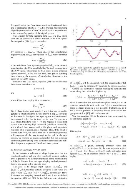
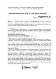
This article has been accepted for publication in a future issue of this journal, but has not been fully edited. Content may change prior to final publication.4It is worth noting that ˜r and ˜ω are non-linear functions of time,and ˜ω approaches infinity at t = 0. For practical reasons duringdigital implementation of the CLV spiral, t = 0 is approximatedwith t = sampling period of the digital system.The equation for total scanning time ˜t total of a CLV spiralscan can be derived in a similar manner to the CAV spiral.From equation (11), ˜t total is derived as˜t total = πr2 endPv . (15)By choosing v = ˜ω end r end where ˜ω end is the instantaneousangular velocity at r end , the equation for ˜t total can be rewrittenas˜t total = πr endP˜ω end. (16)It can be inferred from equation (16) that if ˜ω end = ω, the totalscanning time of a CLV spiral is half of the total scanning timeof a CAV spiral. This makes the CLV spiral a more attractiveoption. However, as we will see later, this gain in scanningtime comes at the expense of introducing distortion at thecenter of the AFM image.Similar to the CAV spiral, equation (13) can be describedin cartesian coordinates asand˜x s = ˜r cos ˜θ (17)ỹ s = ˜r sin ˜θ (18)where ˜θ for time varying ˜ω is obtained as√4πv˜θ = t. (19)PFig. 4 illustrates the input signals ˜x s and ỹ s that can be used togenerate a spiral similar to the one shown in Fig. 2. However,as illustrated in the figure, the input signals are implementedin a reversed order, that is from r end to r start . To generate aCLV spiral, that starts from ˜r = 0, one requires a closed-loopsystem with extremely high bandwidth (ideally ∞ bandwidth)and a closed loop system with a flat phase and magnituderesponse. This of course, is not practical. Thus, if the spiral isstarted from ˜r = 0, the initial error that is inevitably generatedwill propagate all the way through to the end. In the nextsection, we propose an inversion algorithm that can minimizethe tracking error arising from the limited bandwidth and nonidealfrequency response of the closed loop system.C. Inversion Technique for CLV spiralIn this section a technique to shape inputs such that theresulting trajectory will be a CLV spiral with minimal trackingerror is presented. As the implementation of the entire schemewill be in discrete time, the input shaping method presentedhere is also described in discrete time.The goal is to design input signals {u x [k]} N k=0 and{uy [k] } Nsuch that their outputs, along the x and y axes are,k=0{x[k] = ˜x(kT)} N k=0 and {y[k] = ỹ(kT)}N k=0 respectively. Here,T denotes the sampling interval and ˜x and ỹ are as definedin equations (17) and (18). In the following only designing˜xs (µm)ỹs (µm)630360 0.02 0.04 0.06t (s)(b)6303(a)60 0.02 0.04 0.06t (s)Figure 4. Input signals to be applied to the scanner in the x and y axes ofthe scanner to generate CLV spiral scan with v = 1.13 mm/sec (or ˜ω end =188.50 radians/sec). Solid line is the achieved response and dashed line is thedesired trajectory.of {u x [k]} N k=0 will be described, with the understanding that{uy [k] } Ncan be generated by adopting the same procedure.k=0Assume that the transfer function relating the input and theoutput along the x direction is given byG x (z) =b 0 + b 1 z −1 + b 2 z −2 +...+b m z −m1+a 1 z −1 + a 2 z −2 , (20)+...+a m z−m which is stable but has non-minimum phase zeros, i.e. all ofzeros are outside the unit circle. As G x (z) is non-minimumphase, a direct inversion is not possible. Furthermore, as ˜xand ỹ are not periodic, a frequency domain inversion of thetype presented in [15] will not be accurate.Note that equation (20) in the discrete time corresponds tothe difference equationThis impliesx[n]+a 1 x[n − 1]+...+a m x[n − m]= b 0 u x [n]+b 1 u x [n − 1]+...+b m u x [n − m]. (21)u x [n − m] = 1b m(x[n]+a 1 x[n − 1]+...+a m x[n − m]−b n u x [n] −... − b m−1 u x [n −(m − 1)]). (22)As {x[k]} N k=0 is given, assuming arbitrary values foru x [N],u x [N −1],...,u x [N −(m−1)], the input sequence u x [N −(m−1)],u x [N −(m−2)],...,u x [1],u x [0] can be calculated fromequation (22). As an example consider m = 2 in (21). Thisimpliesandx[n]+a 1 x[n − 1]+a 2 x[n − 2]= b 0 u x [n]+b 1 u x [n − 1]+b 2 u x [n − 2] (23)u x [n − 2] = 1 b 2(x[n]+a 1 x[n − 1]+a 2 x[n − 2] − b 0 u x [n] − b 1 u x [n − 1]). (24)Copyright (c) 2009 IEEE. Personal use is permitted. For any other purposes, Permission must be obtained from the IEEE by emailing pubs-permissions@ieee.org.Authorized licensed use limited to: University of Newcastle. Downloaded on November 26, 2009 at 00:02 from IEEE Xplore. Restrictions apply.