timberland investments in an institutional portfolio - Iwc.dk

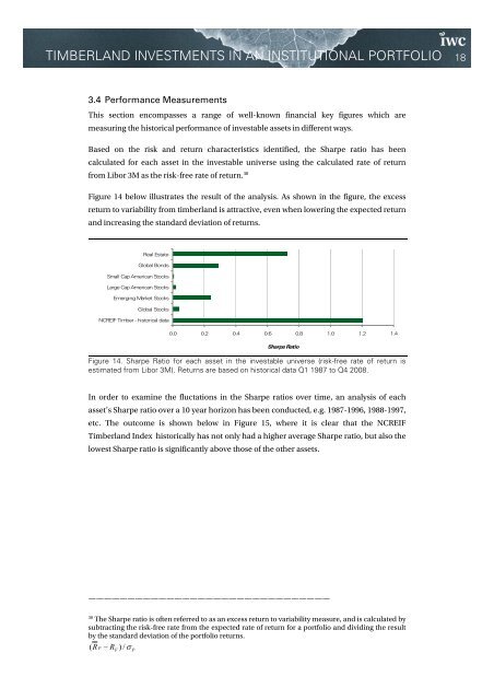
TIMBERLAND INVESTMENTS IN AN INSTITUTIONAL PORTFOLIO 183.4 Performance MeasurementsThis section encompasses a range of well-known financial key figures which aremeasuring the historical performance of investable assets in different ways.Based on the risk and return characteristics identified, the Sharpe ratio has beencalculated for each asset in the investable universe using the calculated rate of returnfrom Libor 3M as the risk-free rate of return. 30Figure 14 below illustrates the result of the analysis. As shown in the figure, the excessreturn to variability from timberland is attractive, even when lowering the expected returnand increasing the standard deviation of returns.Real EstateGlobal BondsSmall Cap American StocksLarge Cap American StocksEmerging Market StocksGlobal StocksNCREIF Timber - historical data0.0 0.2 0.4 0.6 0.8 1.0 1.2 1.4Sharpe RatioFigure 14. Sharpe Ratio for each asset in the investable universe (risk-free rate of return isestimated from Libor 3M). Returns are based on historical data Q1 1987 to Q4 2008.In order to examine the fluctations in the Sharpe ratios over time, an analysis of eachasset’s Sharpe ratio over a 10 year horizon has been conducted, e.g. 1987-1996, 1988-1997,etc. The outcome is shown below in Figure 15, where it is clear that the NCREIFTimberland Index historically has not only had a higher average Sharpe ratio, but also thelowest Sharpe ratio is significantly above those of the other assets.———————————————————————————————30The Sharpe ratio is often referred to as an excess return to variability measure, and is calculated bysubtracting the risk-free rate from the expected rate of return for a portfolio and dividing the resultby the standard deviation of the portfolio returns.( R − ) / σP R FP