DynaPro NanoStar manual - Department of Physiology and Biophysics

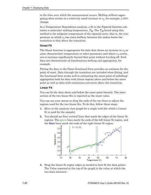
Chapter 7: Displaying Datato the time over which the measurement occurs. Melting without aggregatingoften results in a relatively small increase in r h , for example, a 25%change.In a Temperature Dependence analysis, a fit to the Sigmoid function estimatesa molecular melting temperature, T M . The T M found using thismethod is the midpoint temperature of the sigmoid curve, that is, the temperatureat which r h has risen halfway between the radius below thetransition to that above the transition.Onset FitThe Onset function is appropriate for data that shows an increase in r h atsome characteristic temperature or other parameter and where r h continuesto increase significantly beyond that point without leveling off. Suchdata are characteristic of simultaneous melting and aggregation, forexample.Fitting the data to the Onset functional form provides an estimate for thepoint of onset. Data through the transition are included when fitting, andthe functional form works well in estimating the onset point of unfolding/aggregation both for data with linear regions above and below the onsetpoint as well as data with continuous curvature above the transition.Linear FitYou can fit the data above and below the onset point linearly. The intersectionof the two linear fits is reported as the onset value.You can use your mouse to drag the ends of the two lines to adjust theregions used for the two linear fits. To do this, follow these steps:1. Move to the analysis view graph for a single well (for which a Linearfit is used for the sample).2. You should see four vertical lines that mark the edges of the linear fitregions. The green lines mark the ends of the left linear fit region, andthe blue lines mark the ends of the right linear fit region.3. Drag the linear fit region edges as needed to best fit the data points.The Value reported at the top of the graph is the value at which thetwo lines intersect.7-40 DYNAMICS User’s Guide (M1400 Rev. K)