application of real options valuation to r&d investments in ...

More documents

Recommendations

Info

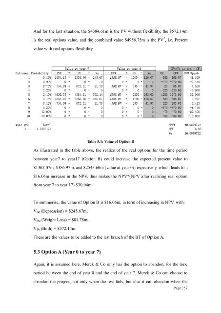
And for the last situation, the $4384.61m is the PV without flexibility, the $572.14mis the real options value, and the combined value $4956.75m is the PV * , i.e. Presentvalue with real options flexibility.Table 5.1: Value of Option BAs illustrated in the table above, the realize of the real options for the time periodbetween year7 to year17 (Option B) could increase the expected present value to$1362.07m, $386.97m, and $2543.60m (value at year 0) respectively, which leads to a$16.06m increase in the NPV, thus makes the NPV*(NPV after realizing real optionfrom year 7 to year 17) $30.04m.To summerise, the value of Option B is $16.06m, in term of increasing in NPV, with:V Bd (Depression) = $245.67m;V Bw (Weight Loss) = $81.78m;V Bb (Both) = $572.14m.These are the values to be added to the last branch of the BT of Option A.5.3 Option A (Year 0 to year 7)Again, it is assumed here, Merck & Co only has the option to abandon, for the timeperiod between the end of year 0 and the end of year 7. Merck & Co can choose toabandon the project, not only when the test fails, but also it can abandon when thePage | 52
project turns out to be unprofitable.The first option is at the end of year 2, when Merck & Co. can choose whether or notto abandon. The second is at the end of year 4, and the third is at the end of year 7. Asall the options can only be exercised at a specific time (i.e. when the Phase ends), itcan be seen as a European option. Moreover, since the third option only exist if thesecond option is open, and the second only exist when the first option is open, theycan be seen as a sequential compound option.Furthermore, as there are two kind of uncertainty regarding to this option, it can beseen as a compound rainbow option. The valuation of a compound rainbow option canbe calculated from a binomial tree approach. However, as result of the complexity ofthis compound option, the valuation of this compound rainbow option can be ratherdifficult. As will see later, there are three underlying assets, which have five differentprobabilities of success for Phase III, and recombined as three probabilities at Phase II,it would be very complicated to construct a single binomial tree in order to value thiscompound rainbow option. Therefore, firstly, a simpler valuation approach is used, byvaluing three separate compound options individually, and then combining the valueusing their corresponding probabilities. After this valuation, the compound rainbowoption is valued by using a single binomial tree to compare the different results.5.3.1 Five variables that determine the value of the optionsThe value of the underlying asset – there are three underlying asset in this case,which are $1200m, $345m, and $2250m respectively.The time to expiration – in this case, as it is a compound option, T 1 is 2, T 2 is 2, andT 3 is 3.Volatility – as mentioned earlier, for the time period between year 0 and year 7, thevolatility would be more project-related. In this case, past performance of LABPharmaceuticals can also be used as a reference. Here, volatility could be calculatedusing the basic formula for standard deviation, and then transferred to yearly volatilityPage | 53
Page 1 and 2:
APPLICATION OF REAL OPTIONS VALUATI
Page 3 and 4:
Table of ContentsAbstract .........
Page 5 and 6:
List of TablesTable 5.1: Value of O
Page 7 and 8: Chapter One— IntroductionAs one o
Page 9 and 10: Then, in Chapter 4, the case study
Page 11 and 12: and we will have the right to take
Page 13 and 14: project, to get its salvage value,
Page 15 and 16: The option to switch:If assets have
Page 17 and 18: 2.2 Advantages of Real Option Valua
Page 19 and 20: In the case of pharmaceutical R&D,
Page 21 and 22: delayed in time. Undertaking one pr
Page 23 and 24: Figure 2.2: Advantages and disadvan
Page 25 and 26: smallest possible payoff of zero, w
Page 27 and 28: options applications is the binomia
Page 29 and 30: t: years to expirationr: annual ris
Page 31 and 32: Chapter Three— Apply Real options
Page 33 and 34: on Howell et al (2001).3.1.1 Precli
Page 35 and 36: approved.3.2 real options valuation
Page 37 and 38: Figure 3.3: Comparison of a call op
Page 39 and 40: applying the principals of activity
Page 41 and 42: that has occurred in the past. Depe
Page 43 and 44: Chapter Four— Case StudyFor this
Page 45 and 46: 4.3 DavanrikLAB Pharmaceuticals ori
Page 47 and 48: efficacious for depression only, a
Page 49 and 50: Chapter Five— Case Study Analysis
Page 51 and 52: figure below:Figure 5.3: NPV of Dav
Page 53 and 54: Merck & Co (10%), which gives $2338
Page 55 and 56: approval and other issues. Therefor
Page 57: of $345m at year 0 (which is $672.3
Page 61 and 62: these three options, the risk-free
Page 63 and 64: ewrite as, noting all the costs (in
Page 65 and 66: Figure 5.10: Valuation of Option A
Page 67 and 68: Figure 5.12: Valuation of Option A
Page 69 and 70: Figure 5.13 Valuation of Compound r
Page 71 and 72: $ in millionmillion to $113.97 mill
Page 73 and 74: Chapter Six— Limitations and conc
Page 75 and 76: discovery projects, arrives in a di
Page 77 and 78: References1. Amram M & Kulatilaka N
Page 79 and 80: 31/08/2006, available at: http://ho
Page 81 and 82: 46. T rigeorgis L . (1995), ―M et
show all

application of real options valuation to r&d investments in ...

You also want an ePaper? Increase the reach of your titles

Delete template?

Save as template?