Introduction to Krylov subspace methods - IMAGe

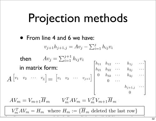
v w.r.t. A is the endConsequence lowest degree monic polynomial ⎡e grade always equal or smaller than m.R m×m of a vector v, v ∈ m w.r.t. A is the lowest degree hmonic polynomial)v = 0. For ADef. ∈ RThe m×m , we grade , vhave ∈of Ra m that vector , we have the v w.r.t. grade thatA the 11 hisof the grade v 12 hlowest is 21 · · · hh 22of degree v is monic polysmaller p(≠ Consequence1) than dim(K m.Projection0) s.t. m ]1j· ·(A; p(A)v v)) = 0. = For min(m, A ∈ Rmethodsm×mgrade(v)), h 21 ∈ R m h, 22 we have that the gradeor smaller than m.alwaysAv equal j =1) dim(K m or smaller[v 1 than v 2 m. · · · v j+1 0· · · hh 32j · ·]nce Av Consequence j =[v 1 (A; vv)) 2 = · · min(m, · v j+1 grade(v))0 h 32 · · · h 0 2j ·· ; v))2)= min(m,(∗)grade(v))0 ⎢ · · ·rade(v)) 2) 1) (∗) dim(K m (A; v)) = min(m, grade(v))⎢ ⎣⎣h j+1,j ·rade of a vector v w.r.t. A is the lowest degree monic polynomialp(A)v = 0. For A ∈ R m×m , v ∈ R m , we have that the grade of v ism (A; v)) = min(m, grade(v))• From line 4 and 6 we have:Notice that v j+1 h j+1,j = Av j − ∑ ji=1 h ijv i . Then Av j =2) (∗)Notice that v j+1 h j+1,j = Av j − ∑ ji=1 h ijv i . Then Av j = ∑ j+1i=1vh ∑Notice that v j+1 h j+1,jj ⎡i=1 h ijv then i . Then Av j = ∑ = Av j − ∑ jj+1i=1 h i=1 h ijv i . Then Av j = ∑ j+1j+1 h j+1,j = Av j − ∑ ji=1 h ijv i . Then Av j j+1j+1,j = Av j − ∑ ji=1 h ijv i . Then Av j = ∑ 0LOV SUBSPACE METHODSj+1i=1 h i=1 ijv i :⎡ ⎡i=1 h ijv i⎡:⎡ ⎡ijv i : ⎡ ⎤h 11h ∗ ∗ 11 h 12h · · · 12 · · · ⎤· · ∗·hh 1j11 h 11 h 12 h 12 · · · · h 1j h 11· · ·h 12 · · · h 1j ·⎡in matrix form:5 KRYLOV SUBSPACE⎡⎤h 21 h 22 · h h 21 h h 2jh 11 h 12 · · · 1j · · · ]22 · · · h 2j · · ·]21 h 21 h 22 h 22 · · · h 2j · · ·h METHODS 0 ∗ · ·21 h ⎤⎡ ]⎤]]j =[v 1 v 2 j+1 0 h 32 · h 2jAv h 21 h 22 j · · vh 2 v 2j · j+1 0 h 32 · · · h 2j · · ·Av j =1 v 2 · · v j+1 0 h 32 · 2j =[v 1 v 2 · · · v j+1 0 h 32 · · h 2j · · ·]]∗ ∗ · 22 · · · · 0·∗1 ]· · · 0A[v 1 v 2 · · · v m =.[v 1 v 2 · · · v m+1 Av j =0 · ·[v 0 ·· · ·]0 v 2 · · · · · · j+1 0 ] ..0 ∗ h· 32· · · · · ∗A[v 1 v 2 · · · v1 m =[v 10v 2 · · ⎢· ⎢ v m+1 V.m = Vm ⎥T V m+1 H m =. ⎢v ⎣h j+1j+1 0 h 32 ·⎢· · h.2j · · h·⎣h j+1,j · · ⎦j+1,j j+1,j · · ·⎥⎦⎣ ⎡ 0 .. · · ∗·⎣ .. ⎥0 .. ∗0⎦1 ⎢· · ·⎢ . 0 · · ·0⎣.. ⎥⎣ 01 0⎢⎡ ⎥⎡1 ∗ ∗⎦⎤ 0: AV m ⎡⎣= V m+1 H m hVj+1,jm T AV ∗ m ∗ · = ⎦V· T m×(m+1)m V m+1 ⎤ H∗ m = ∗ · · · ∗∗ ∗ · · · ∗ ⎢ 0 ⎡ . ∗0 ∗ · · · ∗ ∗· · ·] ]0 ∗ · ⎣ .. 0]0 ∗ · · · ∗]. : VAV A[v 1 v 0 · · ·[ ⎡2 · v m =[v 1 v . 2 · · · v] [ ⎤m+1 0 ..⎡m T AV 2 · · ·] mv[ m = VH m = m+1 m where H mH [v 1 v 2 · · v] m := {H m deleted the last row}m+1 0 .. . ⎢· · v = v v · · · v ⎢ 0 .. ∗ ∗ 1ark : In practice, a modified Gram-Schmidt ∗(MGS) ⎥ ⎢ is used ] ⎢ on the ⎥ Ho 32⎢.