- Page 2:
Introduction to Nonextensive Statis
- Page 6:
Constantino TsallisCentro Brasileir
- Page 10:
PrefaceIn 1902, after three decades
- Page 14:
Prefaceixequation inspired by the p
- Page 18:
Prefacexinearby. 4 Nonextensive sta
- Page 22:
Prefacexiiicircular epicycles. So w
- Page 26:
ContentsPart IBasics or How the The
- Page 30:
Contentsxvii5.2 Low-Dimensional Con
- Page 34:
Part IBasics or How the Theory Work
- Page 38:
4 1 Historical Background and Physi
- Page 42:
6 1 Historical Background and Physi
- Page 46:
8 1 Historical Background and Physi
- Page 50:
10 1 Historical Background and Phys
- Page 54:
12 1 Historical Background and Phys
- Page 58:
14 1 Historical Background and Phys
- Page 62:
16 1 Historical Background and Phys
- Page 66:
Chapter 2Learning with Boltzmann-Gi
- Page 70:
2.1 Boltzmann-Gibbs Entropy 212.1.2
- Page 74:
2.1 Boltzmann-Gibbs Entropy 232.1.2
- Page 78:
2.1 Boltzmann-Gibbs Entropy 25where
- Page 82:
2.1 Boltzmann-Gibbs Entropy 27the s
- Page 86:
2.2 Kullback-Leibler Relative Entro
- Page 90:
2.3 Constraints and Entropy Optimiz
- Page 94:
2.4 Boltzmann-Gibbs Statistical Mec
- Page 98:
2.4 Boltzmann-Gibbs Statistical Mec
- Page 102:
Chapter 3Generalizing What We Learn
- Page 106:
3.1 Playing with Differential Equat
- Page 110:
3.2 Nonadditive Entropy S q 41We sh
- Page 114:
3.2 Nonadditive Entropy S q 43This
- Page 118:
3.2 Nonadditive Entropy S q 453.2.2
- Page 122:
3.2 Nonadditive Entropy S q 47we ca
- Page 126:
3.2 Nonadditive Entropy S q 49S BG
- Page 130:
3.2 Nonadditive Entropy S q 51with
- Page 134:
3.2 Nonadditive Entropy S q 53whose
- Page 138:
3.3 Correlations, Occupancy of Phas
- Page 142:
3.3 Correlations, Occupancy of Phas
- Page 146:
3.3 Correlations, Occupancy of Phas
- Page 150:
3.3 Correlations, Occupancy of Phas
- Page 154:
3.3 Correlations, Occupancy of Phas
- Page 158:
3.3 Correlations, Occupancy of Phas
- Page 162:
3.3 Correlations, Occupancy of Phas
- Page 166:
3.3 Correlations, Occupancy of Phas
- Page 170:
3.3 Correlations, Occupancy of Phas
- Page 174:
3.3 Correlations, Occupancy of Phas
- Page 178:
3.3 Correlations, Occupancy of Phas
- Page 182:
3.3 Correlations, Occupancy of Phas
- Page 186:
3.3 Correlations, Occupancy of Phas
- Page 190:
3.3 Correlations, Occupancy of Phas
- Page 194:
3.3 Correlations, Occupancy of Phas
- Page 198:
3.4 q-Generalization of the Kullbac
- Page 202:
3.4 q-Generalization of the Kullbac
- Page 206:
3.5 Constraints and Entropy Optimiz
- Page 210:
3.6 Nonextensive Statistical Mechan
- Page 214:
3.6 Nonextensive Statistical Mechan
- Page 218:
3.6 Nonextensive Statistical Mechan
- Page 222:
3.6 Nonextensive Statistical Mechan
- Page 226:
3.7 About the Escort Distribution a
- Page 230:
3.7 About the Escort Distribution a
- Page 234:
3.8 About Universal Constants in Ph
- Page 238:
3.9 Various Other Entropic Forms 10
- Page 242:
Part IIFoundations or Why the Theor
- Page 246:
110 4 Stochastic Dynamical Foundati
- Page 250:
112 4 Stochastic Dynamical Foundati
- Page 254:
114 4 Stochastic Dynamical Foundati
- Page 258:
116 4 Stochastic Dynamical Foundati
- Page 262:
118 4 Stochastic Dynamical Foundati
- Page 266:
120 4 Stochastic Dynamical Foundati
- Page 270:
122 4 Stochastic Dynamical Foundati
- Page 274:
124 4 Stochastic Dynamical Foundati
- Page 278:
126 4 Stochastic Dynamical Foundati
- Page 282:
128 4 Stochastic Dynamical Foundati
- Page 286:
130 4 Stochastic Dynamical Foundati
- Page 290:
132 4 Stochastic Dynamical Foundati
- Page 294:
134 4 Stochastic Dynamical Foundati
- Page 298:
136 4 Stochastic Dynamical Foundati
- Page 302:
138 4 Stochastic Dynamical Foundati
- Page 306:
140 4 Stochastic Dynamical Foundati
- Page 310:
142 4 Stochastic Dynamical Foundati
- Page 314:
144 4 Stochastic Dynamical Foundati
- Page 318:
146 4 Stochastic Dynamical Foundati
- Page 322:
148 4 Stochastic Dynamical Foundati
- Page 326:
150 4 Stochastic Dynamical Foundati
- Page 330:
152 5 Deterministic Dynamical Found
- Page 334:
154 5 Deterministic Dynamical Found
- Page 338:
156 5 Deterministic Dynamical Found
- Page 342:
158 5 Deterministic Dynamical Found
- Page 346:
160 5 Deterministic Dynamical Found
- Page 350:
162 5 Deterministic Dynamical Found
- Page 354:
164 5 Deterministic Dynamical Found
- Page 358:
166 5 Deterministic Dynamical Found
- Page 362:
10 -5 1 10 100 100010 -5 1 10 100 1
- Page 366:
170 5 Deterministic Dynamical Found
- Page 370:
172 5 Deterministic Dynamical Found
- Page 374:
174 5 Deterministic Dynamical Found
- Page 378:
176 5 Deterministic Dynamical Found
- Page 382:
178 5 Deterministic Dynamical Found
- Page 386:
180 5 Deterministic Dynamical Found
- Page 390:
182 5 Deterministic Dynamical Found
- Page 394:
184 5 Deterministic Dynamical Found
- Page 398:
186 5 Deterministic Dynamical Found
- Page 402:
188 5 Deterministic Dynamical Found
- Page 406:
190 5 Deterministic Dynamical Found
- Page 410:
192 5 Deterministic Dynamical Found
- Page 414:
194 5 Deterministic Dynamical Found
- Page 418:
196 5 Deterministic Dynamical Found
- Page 422:
198 5 Deterministic Dynamical Found
- Page 426:
200 5 Deterministic Dynamical Found
- Page 430:
202 5 Deterministic Dynamical Found
- Page 434:
204 5 Deterministic Dynamical Found
- Page 438:
206 5 Deterministic Dynamical Found
- Page 442:
Chapter 6Generalizing Nonextensive
- Page 446:
6.2 Further Generalizing 211dydx =
- Page 450:
6.2 Further Generalizing 213∫ W{
- Page 454:
6.2 Further Generalizing 215Then, f
- Page 458:
6.2 Further Generalizing 217If f (
- Page 462:
Part IIIApplications or What for th
- Page 466:
222 7 Thermodynamical and Nonthermo
- Page 470:
224 7 Thermodynamical and Nonthermo
- Page 474:
226 7 Thermodynamical and Nonthermo
- Page 478:
228 7 Thermodynamical and Nonthermo
- Page 482:
230 7 Thermodynamical and Nonthermo
- Page 486:
232 7 Thermodynamical and Nonthermo
- Page 490:
234 7 Thermodynamical and Nonthermo
- Page 494:
236 7 Thermodynamical and Nonthermo
- Page 498:
238 7 Thermodynamical and Nonthermo
- Page 502:
240 7 Thermodynamical and Nonthermo
- Page 506:
242 7 Thermodynamical and Nonthermo
- Page 510:
244 7 Thermodynamical and Nonthermo
- Page 514:
246 7 Thermodynamical and Nonthermo
- Page 518:
248 7 Thermodynamical and Nonthermo
- Page 522:
250 7 Thermodynamical and Nonthermo
- Page 526:
252 7 Thermodynamical and Nonthermo
- Page 530:
254 7 Thermodynamical and Nonthermo
- Page 534:
256 7 Thermodynamical and Nonthermo
- Page 538:
258 7 Thermodynamical and Nonthermo
- Page 542: 260 7 Thermodynamical and Nonthermo
- Page 546: 262 7 Thermodynamical and Nonthermo
- Page 550: 264 7 Thermodynamical and Nonthermo
- Page 554: 266 7 Thermodynamical and Nonthermo
- Page 558: 268 7 Thermodynamical and Nonthermo
- Page 562: 270 7 Thermodynamical and Nonthermo
- Page 566: 272 7 Thermodynamical and Nonthermo
- Page 570: 274 7 Thermodynamical and Nonthermo
- Page 574: 276 7 Thermodynamical and Nonthermo
- Page 578: 278 7 Thermodynamical and Nonthermo
- Page 582: 280 7 Thermodynamical and Nonthermo
- Page 586: 282 7 Thermodynamical and Nonthermo
- Page 590: 284 7 Thermodynamical and Nonthermo
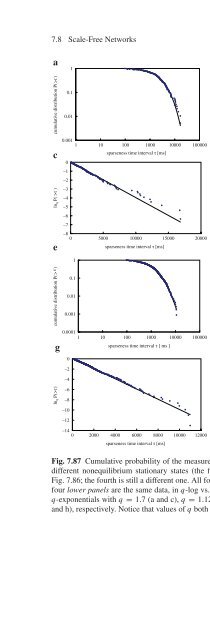
- Page 596: 7.8 Scale-Free Networks 287Fig. 7.9
- Page 600: 7.8 Scale-Free Networks 289Fig. 7.9
- Page 604: 7.8 Scale-Free Networks 291Fig. 7.9
- Page 608: 7.8 Scale-Free Networks 293Fig. 7.9
- Page 612: 7.10 Other Sciences 295Fig. 7.102 S
- Page 616: 7.10 Other Sciences 297Fig. 7.105 F
- Page 620: 7.10 Other Sciences 299Fig. 7.109 Z
- Page 624: 7.10 Other Sciences 301Fig. 7.112 C
- Page 628: Chapter 8Final Comments and Perspec
- Page 632: 8.1 Falsifiable Predictions and Con
- Page 636: 8.2 Frequently Asked Questions 309i
- Page 640: 8.2 Frequently Asked Questions 311B
- Page 644:
8.2 Frequently Asked Questions 313(
- Page 648:
8.2 Frequently Asked Questions 315o
- Page 652:
8.2 Frequently Asked Questions 317p
- Page 656:
8.2 Frequently Asked Questions 319n
- Page 660:
8.2 Frequently Asked Questions 321L
- Page 664:
8.2 Frequently Asked Questions 323(
- Page 668:
8.2 Frequently Asked Questions 3254
- Page 672:
8.3 Open Questions 327This is a fre
- Page 676:
330 Appendix A Useful Mathematical
- Page 680:
332 Appendix A Useful Mathematical
- Page 684:
334 Appendix A Useful Mathematical
- Page 688:
336 Appendix B Escort Distributions
- Page 692:
338 Appendix B Escort Distributions
- Page 696:
340 Appendix B Escort Distributions
- Page 700:
Bibliography1. J.W. Gibbs, Elementa
- Page 704:
Bibliography 34541. A. Rapisarda an
- Page 708:
Bibliography 34784. A.N. Kolmogorov
- Page 712:
Bibliography 349123. T. Schneider,
- Page 716:
Bibliography 351178. A. Campa, A. G
- Page 720:
Bibliography 353230. S. Abe and A.K
- Page 724:
Bibliography 355279. K. Briggs and
- Page 728:
Bibliography 357329. T. Kodama, H.-
- Page 732:
Bibliography 359Italy), eds. C. Bec
- Page 736:
Bibliography 361431. M.J.A. Bolzan,
- Page 740:
Bibliography 363479. T. Cattaert, M
- Page 744:
Bibliography 365528. P.H. Chavanis,
- Page 748:
Bibliography 367579. G.A. Tsekouras
- Page 752:
Bibliography 369631. J. Schulte, No
- Page 756:
Bibliography 371678. D. Fuks, S. Do
- Page 760:
Bibliography 373723. L.J. Yang, M.P
- Page 764:
Bibliography 375767. S. Sun, L. Zha
- Page 768:
Bibliography 377813. S. Abe, Tsalli
- Page 772:
Bibliography 379862. S. Boccaletti,
- Page 776:
382 IndexKekule, ixKepler, xiiKrylo