- Page 2:
Introduction to Nonextensive Statis
- Page 6:
Constantino TsallisCentro Brasileir
- Page 10:
PrefaceIn 1902, after three decades
- Page 14:
Prefaceixequation inspired by the p
- Page 18:
Prefacexinearby. 4 Nonextensive sta
- Page 22:
Prefacexiiicircular epicycles. So w
- Page 26:
ContentsPart IBasics or How the The
- Page 30:
Contentsxvii5.2 Low-Dimensional Con
- Page 34:
Part IBasics or How the Theory Work
- Page 38:
4 1 Historical Background and Physi
- Page 42: 6 1 Historical Background and Physi
- Page 46: 8 1 Historical Background and Physi
- Page 50: 10 1 Historical Background and Phys
- Page 54: 12 1 Historical Background and Phys
- Page 58: 14 1 Historical Background and Phys
- Page 62: 16 1 Historical Background and Phys
- Page 66: Chapter 2Learning with Boltzmann-Gi
- Page 70: 2.1 Boltzmann-Gibbs Entropy 212.1.2
- Page 74: 2.1 Boltzmann-Gibbs Entropy 232.1.2
- Page 78: 2.1 Boltzmann-Gibbs Entropy 25where
- Page 82: 2.1 Boltzmann-Gibbs Entropy 27the s
- Page 86: 2.2 Kullback-Leibler Relative Entro
- Page 90: 2.3 Constraints and Entropy Optimiz
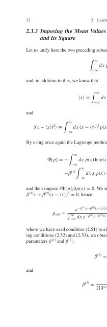
- Page 96: 34 2 Learning with Boltzmann-Gibbs
- Page 100: 36 2 Learning with Boltzmann-Gibbs
- Page 104: 38 3 Generalizing What We Learntwho
- Page 108: 40 3 Generalizing What We Learnt1e
- Page 112: 42 3 Generalizing What We Learnt3q
- Page 116: 44 3 Generalizing What We Learntas
- Page 120: 46 3 Generalizing What We LearntFig
- Page 124: 48 3 Generalizing What We LearntFig
- Page 128: 50 3 Generalizing What We LearntLet
- Page 132: 52 3 Generalizing What We Learnt(i)
- Page 136: 54 3 Generalizing What We Learntin
- Page 140: 56 3 Generalizing What We Learntran
- Page 144:
58 3 Generalizing What We Learntg(T
- Page 148:
60 3 Generalizing What We LearntThe
- Page 152:
62 3 Generalizing What We Learnt1/(
- Page 156:
64 3 Generalizing What We LearntFig
- Page 160:
66 3 Generalizing What We LearntLet
- Page 164:
68 3 Generalizing What We LearntThe
- Page 168:
70 3 Generalizing What We LearntTab
- Page 172:
72 3 Generalizing What We LearntTab
- Page 176:
74 3 Generalizing What We Learnt100
- Page 180:
76 3 Generalizing What We Learntpro
- Page 184:
78 3 Generalizing What We Learnt100
- Page 188:
80 3 Generalizing What We Learnt0.0
- Page 192:
82 3 Generalizing What We Learntspi
- Page 196:
84 3 Generalizing What We Learnt0.8
- Page 200:
86 3 Generalizing What We LearntThi
- Page 204:
88 3 Generalizing What We Learnt1 (
- Page 208:
90 3 Generalizing What We Learntwhe
- Page 212:
92 3 Generalizing What We LearntIf
- Page 216:
94 3 Generalizing What We LearntBec
- Page 220:
96 3 Generalizing What We Learntwhe
- Page 224:
98 3 Generalizing What We Learntste
- Page 228:
100 3 Generalizing What We Learntq-
- Page 232:
102 3 Generalizing What We Learntwh
- Page 236:
104 3 Generalizing What We Learntth
- Page 240:
106 3 Generalizing What We LearntTa
- Page 244:
Chapter 4Stochastic Dynamical Found
- Page 248:
4.4 Correlated Anomalous Diffusion
- Page 252:
4.4 Correlated Anomalous Diffusion
- Page 256:
4.4 Correlated Anomalous Diffusion
- Page 260:
4.5 Stable Solutions of Fokker-Plan
- Page 264:
4.6 Probabilistic Models with Corre
- Page 268:
4.6 Probabilistic Models with Corre
- Page 272:
4.6 Probabilistic Models with Corre
- Page 276:
4.6 Probabilistic Models with Corre
- Page 280:
4.6 Probabilistic Models with Corre
- Page 284:
4.6 Probabilistic Models with Corre
- Page 288:
4.6 Probabilistic Models with Corre
- Page 292:
4.6 Probabilistic Models with Corre
- Page 296:
4.7 Central Limit Theorems 135Fig.
- Page 300:
4.7 Central Limit Theorems 137See F
- Page 304:
4.7 Central Limit Theorems 139Fig.
- Page 308:
4.7 Central Limit Theorems 141Fig.
- Page 312:
4.7 Central Limit Theorems 143Fig.
- Page 316:
4.8 Generalizing the Langevin Equat
- Page 320:
4.8 Generalizing the Langevin Equat
- Page 324:
4.9 Time-Dependent Ginzburg-Landau
- Page 328:
Chapter 5Deterministic Dynamical Fo
- Page 332:
5.1 Low-Dimensional Dissipative Map
- Page 336:
5.1 Low-Dimensional Dissipative Map
- Page 340:
5.1 Low-Dimensional Dissipative Map
- Page 344:
5.1 Low-Dimensional Dissipative Map
- Page 348:
5.1 Low-Dimensional Dissipative Map
- Page 352:
5.1 Low-Dimensional Dissipative Map
- Page 356:
5.2 Low-Dimensional Conservative Ma
- Page 360:
5.2 Low-Dimensional Conservative Ma
- Page 364:
5.2 Low-Dimensional Conservative Ma
- Page 368:
5.2 Low-Dimensional Conservative Ma
- Page 372:
5.2 Low-Dimensional Conservative Ma
- Page 376:
5.2 Low-Dimensional Conservative Ma
- Page 380:
5.2 Low-Dimensional Conservative Ma
- Page 384:
5.3 High-Dimensional Conservative M
- Page 388:
5.3 High-Dimensional Conservative M
- Page 392:
5.4 Many-Body Long-Range-Interactin
- Page 396:
5.4 Many-Body Long-Range-Interactin
- Page 400:
5.4 Many-Body Long-Range-Interactin
- Page 404:
5.4 Many-Body Long-Range-Interactin
- Page 408:
5.5 The q-Triplet 1910.500.48N = 20
- Page 412:
5.5 The q-Triplet 19310 010 -1N = 2
- Page 416:
5.6 Connection with Critical Phenom
- Page 420:
5.7 A Conjecture on the Time and Si
- Page 424:
5.7 A Conjecture on the Time and Si
- Page 428:
5.7 A Conjecture on the Time and Si
- Page 432:
5.7 A Conjecture on the Time and Si
- Page 436:
5.7 A Conjecture on the Time and Si
- Page 440:
p5.7 A Conjecture on the Time and S
- Page 444:
210 6 Generalizing Nonextensive Sta
- Page 448:
212 6 Generalizing Nonextensive Sta
- Page 452:
214 6 Generalizing Nonextensive Sta
- Page 456:
216 6 Generalizing Nonextensive Sta
- Page 460:
218 6 Generalizing Nonextensive Sta
- Page 464:
Chapter 7Thermodynamical and Nonthe
- Page 468:
7.1 Physics 223Fig. 7.1 Computation
- Page 472:
7.1 Physics 225hypergeometric funct
- Page 476:
7.1 Physics 227Fig. 7.6 The dashed
- Page 480:
7.1 Physics 229Fig. 7.7 Example sha
- Page 484:
7.1 Physics 231Fig. 7.11 Experiment
- Page 488:
7.1 Physics 2337.1.4 FingeringWhen
- Page 492:
7.1 Physics 235Fig. 7.16 The vertic
- Page 496:
7.1 Physics 237Fig. 7.19 Measured (
- Page 500:
7.1 Physics 239Fig. 7.23 Time evolu
- Page 504:
7.1 Physics 2417.1.8 Astrophysics7.
- Page 508:
7.1 Physics 243Fig. 7.28 Top: Fits
- Page 512:
7.1 Physics 245Fig. 7.30 Log-Log pl
- Page 516:
7.1 Physics 247Fig. 7.32 Dependence
- Page 520:
7.1 Physics 249Fig. 7.36 Data colla
- Page 524:
7.1 Physics 251Fig. 7.39 Cumulative
- Page 528:
7.1 Physics 253a0-1--2-3-4-5- - - -
- Page 532:
7.1 Physics 2551.25fit in Fig.2Eq.(
- Page 536:
7.1 Physics 2574.0q relc3.53.02.52.
- Page 540:
7.2 Chemistry 259Fig. 7.49 (a) Dime
- Page 544:
7.2 Chemistry 261Fig. 7.52 d = 2(a)
- Page 548:
7.2 Chemistry 263Fig. 7.55 Snapshot
- Page 552:
7.2 Chemistry 265Fig. 7.58 Log-log
- Page 556:
7.3 Economics 267Fig. 7.60 Ground-s
- Page 560:
7.4 Computer Sciences 269Fig. 7.64
- Page 564:
7.4 Computer Sciences 271Fig. 7.67
- Page 568:
7.4 Computer Sciences 273Fig. 7.71
- Page 572:
7.4 Computer Sciences 275Fig. 7.74
- Page 576:
7.4 Computer Sciences 277Fig. 7.77
- Page 580:
7.4 Computer Sciences 279Fig. 7.80
- Page 584:
7.5 Biosciences 281Fig. 7.82 Image
- Page 588:
7.8 Scale-Free Networks 283Fig. 7.8
- Page 592:
7.8 Scale-Free Networks 285a1b1cumu
- Page 596:
7.8 Scale-Free Networks 287Fig. 7.9
- Page 600:
7.8 Scale-Free Networks 289Fig. 7.9
- Page 604:
7.8 Scale-Free Networks 291Fig. 7.9
- Page 608:
7.8 Scale-Free Networks 293Fig. 7.9
- Page 612:
7.10 Other Sciences 295Fig. 7.102 S
- Page 616:
7.10 Other Sciences 297Fig. 7.105 F
- Page 620:
7.10 Other Sciences 299Fig. 7.109 Z
- Page 624:
7.10 Other Sciences 301Fig. 7.112 C
- Page 628:
Chapter 8Final Comments and Perspec
- Page 632:
8.1 Falsifiable Predictions and Con
- Page 636:
8.2 Frequently Asked Questions 309i
- Page 640:
8.2 Frequently Asked Questions 311B
- Page 644:
8.2 Frequently Asked Questions 313(
- Page 648:
8.2 Frequently Asked Questions 315o
- Page 652:
8.2 Frequently Asked Questions 317p
- Page 656:
8.2 Frequently Asked Questions 319n
- Page 660:
8.2 Frequently Asked Questions 321L
- Page 664:
8.2 Frequently Asked Questions 323(
- Page 668:
8.2 Frequently Asked Questions 3254
- Page 672:
8.3 Open Questions 327This is a fre
- Page 676:
330 Appendix A Useful Mathematical
- Page 680:
332 Appendix A Useful Mathematical
- Page 684:
334 Appendix A Useful Mathematical
- Page 688:
336 Appendix B Escort Distributions
- Page 692:
338 Appendix B Escort Distributions
- Page 696:
340 Appendix B Escort Distributions
- Page 700:
Bibliography1. J.W. Gibbs, Elementa
- Page 704:
Bibliography 34541. A. Rapisarda an
- Page 708:
Bibliography 34784. A.N. Kolmogorov
- Page 712:
Bibliography 349123. T. Schneider,
- Page 716:
Bibliography 351178. A. Campa, A. G
- Page 720:
Bibliography 353230. S. Abe and A.K
- Page 724:
Bibliography 355279. K. Briggs and
- Page 728:
Bibliography 357329. T. Kodama, H.-
- Page 732:
Bibliography 359Italy), eds. C. Bec
- Page 736:
Bibliography 361431. M.J.A. Bolzan,
- Page 740:
Bibliography 363479. T. Cattaert, M
- Page 744:
Bibliography 365528. P.H. Chavanis,
- Page 748:
Bibliography 367579. G.A. Tsekouras
- Page 752:
Bibliography 369631. J. Schulte, No
- Page 756:
Bibliography 371678. D. Fuks, S. Do
- Page 760:
Bibliography 373723. L.J. Yang, M.P
- Page 764:
Bibliography 375767. S. Sun, L. Zha
- Page 768:
Bibliography 377813. S. Abe, Tsalli
- Page 772:
Bibliography 379862. S. Boccaletti,
- Page 776:
382 IndexKekule, ixKepler, xiiKrylo