EIB Papers Volume 13. n°1/2008 - European Investment Bank
EIB Papers Volume 13. n°1/2008 - European Investment Bank
EIB Papers Volume 13. n°1/2008 - European Investment Bank

Create successful ePaper yourself
Turn your PDF publications into a flip-book with our unique Google optimized e-Paper software.
Box 1. Burden and excess burden of taxation – conventional approach<br />
Figure B1 illustrates graphically the burden and the excess burden of taxation for a wage tax.<br />
It pictures the demand for and supply of labour – measured in hours worked – as a function<br />
of the wage rate. To be precise, D 0 shows firms’ demand for labour when there is no wage<br />
tax. For simplicity, the demand schedule is assumed to be flat rather than downward sloping.<br />
This implies that the marginal product of labour, which sets the wage firms are willing<br />
to pay, does not fall when firms use more labour. S 0 shows households’ supply of labour.<br />
A change in the supply of labour reflects a change in the hours worked by households already<br />
working (intensive labour-supply response) and a change in the labour force participation<br />
rate (extensive labour-supply response). The link between wages and labour supply is positive<br />
for two related reasons. First, working more comes at the expense of leisure and, second,<br />
the marginal value of leisure forgone rises with successive cuts in leisure. Thus, the wage<br />
households require for working more and cutting leisure rises with an increase in the amount<br />
of time allocated to working, or – equivalently – as wages go up, households wish to allocate<br />
more of their time to work and less to leisure. The labour-supply curve might be steeper or<br />
flatter than the one shown in the diagram. In fact, it might be backward-bending. These issues<br />
will be taken up in Box 3 of Section 4.<br />
The labour-market equilibrium resulting from the interactions between firms and households<br />
yields a wage of BO , hours worked of L 0 and, thus, labour income equivalent to the area OL 0 AB.<br />
As the labour-demand schedule represents the marginal product of labour, this area also<br />
represents workers’ contribution to the value of output, and with constant returns to scale and<br />
in the absence of other factor inputs it equals the value of output. This value can be readily<br />
compared with the economic cost of producing it. This cost is given by the total value of<br />
leisure forgone, which equals the area OL 0 AF under the labour-supply schedule. With the value<br />
of output (OL 0 AB) exceeding the economic cost of generating it (OL 0 AF), there is thus a laboursupply<br />
surplus of FAB. How does introducing a wage tax change this surplus and how does this<br />
change relate to the burden and the excess burden of taxation?<br />
Figure B1. Burden and excess burden of taxation – conventional approach<br />
Wage<br />
B<br />
C<br />
F<br />
O<br />
E A<br />
D<br />
L1<br />
S0<br />
D0<br />
D1<br />
L0 Labour supply and demand<br />
(in hours worked)<br />
A neat way of illustrating the impact of a wage tax assumes that firms make the tax payments<br />
to the government. But as they do not want to foot the bill, they offer households a lower net<br />
(after-tax) wage, and as firms demand for labour is completely elastic, they succeed in passing<br />
<strong>EIB</strong> PAPERS <strong>Volume</strong>13 N°1 <strong>2008</strong> 89