- Page 2:
Chapter 1: Overview and Descriptive
- Page 6:
Chapter 1: Overview and Descriptive
- Page 10:
Chapter 1: Overview and Descriptive
- Page 16:
Chapter 1: Overview and Descriptive
- Page 20:
Chapter 1: Overview and Descriptive
- Page 24:
Chapter 1: Overview and Descriptive
- Page 28:
Chapter 1: Overview and Descriptive
- Page 32:
Chapter 1: Overview and Descriptive
- Page 36:
Chapter 1: Overview and Descriptive
- Page 40:
Chapter 1: Overview and Descriptive
- Page 44:
Chapter 1: Overview and Descriptive
- Page 48:
Chapter 1: Overview and Descriptive
- Page 52:
Chapter 1: Overview and Descriptive
- Page 56:
Chapter 1: Overview and Descriptive
- Page 62:
Chapter 1: Overview and Descriptive
- Page 66:
Chapter 1: Overview and Descriptive
- Page 70:
Chapter 1: Overview and Descriptive
- Page 74:
Chapter 1: Overview and Descriptive
- Page 78:
Chapter 1: Overview and Descriptive
- Page 82:
Chapter 1: Overview and Descriptive
- Page 86:
Chapter 1: Overview and Descriptive
- Page 90:
Chapter 1: Overview and Descriptive
- Page 94:
CHAPTER 2Section 2.11.a. S = { 1324
- Page 98:
Chapter 2: Probability5.a.OutcomeNu
- Page 102:
Chapter 2: Probability8.a. A 1 ∪
- Page 106:
Chapter 2: Probability9.a. In the d
- Page 110:
Chapter 2: Probabilityf. either (ne
- Page 114:
Chapter 2: Probability17.a. The pro
- Page 118:
Chapter 2: Probability24. Since A i
- Page 122:
Chapter 2: ProbabilitySection 2.329
- Page 126:
Chapter 2: Probability34.⎛20⎞
- Page 130:
Chapter 2: Probabilityd. To examine
- Page 134:
Chapter 2: Probability42. Seats:2
- Page 138:
Chapter 2: Probability47.P(A ∩ B)
- Page 142:
Chapter 2: ProbabilityP(M ∩ SS
- Page 146:
Chapter 2: Probabilityc. P(all H’
- Page 150:
Chapter 2: Probability61. P(0 def i
- Page 154:
Chapter 2: Probability63.a.b. P(A
- Page 158:
Chapter 2: Probability66. Define ev
- Page 162:
Chapter 2: ProbabilitySection 2.568
- Page 166:
Chapter 2: Probability79.Using the
- Page 170:
Chapter 2: Probabilityd. P(passes i
- Page 174:
Chapter 2: ProbabilitySupplementary
- Page 178:
Chapter 2: Probability93.1a. There
- Page 182:
Chapter 2: Probability101.a. The la
- Page 186:
Chapter 2: Probabilityd. For what v
- Page 190:
CHAPTER 3Section 3.11.S: FFF SFF FS
- Page 194:
Chapter 3: Discrete Random Variable
- Page 198:
Chapter 3: Discrete Random Variable
- Page 202:
Chapter 3: Discrete Random Variable
- Page 206:
Chapter 3: Discrete Random Variable
- Page 210:
Chapter 3: Discrete Random Variable
- Page 214:
Chapter 3: Discrete Random Variable
- Page 218:
Chapter 3: Discrete Random Variable
- Page 222:
Chapter 3: Discrete Random Variable
- Page 226:
Chapter 3: Discrete Random Variable
- Page 230:
Chapter 3: Discrete Random Variable
- Page 234:
Chapter 3: Discrete Random Variable
- Page 238:
Chapter 3: Discrete Random Variable
- Page 242:
Chapter 3: Discrete Random Variable
- Page 246:
Chapter 3: Discrete Random Variable
- Page 250:
Chapter 3: Discrete Random Variable
- Page 254:
Chapter 3: Discrete Random Variable
- Page 258:
CHAPTER 4Section 4.11.1∫ −∞11
- Page 262:
Chapter 4: Continuous Random Variab
- Page 266:
Chapter 4: Continuous Random Variab
- Page 270:
Chapter 4: Continuous Random Variab
- Page 274:
Chapter 4: Continuous Random Variab
- Page 278:
Chapter 4: Continuous Random Variab
- Page 282:
Chapter 4: Continuous Random Variab
- Page 286:
Chapter 4: Continuous Random Variab
- Page 290:
Chapter 4: Continuous Random Variab
- Page 294:
Chapter 4: Continuous Random Variab
- Page 298:
Chapter 4: Continuous Random Variab
- Page 302:
Chapter 4: Continuous Random Variab
- Page 306:
Chapter 4: Continuous Random Variab
- Page 310:
Chapter 4: Continuous Random Variab
- Page 314:
Chapter 4: Continuous Random Variab
- Page 318:
Chapter 4: Continuous Random Variab
- Page 322:
Chapter 4: Continuous Random Variab
- Page 326: Chapter 4: Continuous Random Variab
- Page 330: Chapter 4: Continuous Random Variab
- Page 334: Chapter 4: Continuous Random Variab
- Page 338: Chapter 4: Continuous Random Variab
- Page 342: Chapter 4: Continuous Random Variab
- Page 346: Chapter 4: Continuous Random Variab
- Page 350: CHAPTER 5Section 5.11.a. P(X = 1, Y
- Page 354: Chapter 5: Joint Probability Distri
- Page 358: Chapter 5: Joint Probability Distri
- Page 362: Chapter 5: Joint Probability Distri
- Page 366: Chapter 5: Joint Probability Distri
- Page 370: Chapter 5: Joint Probability Distri
- Page 374: Chapter 5: Joint Probability Distri
- Page 380: Chapter 5: Joint Probability Distri
- Page 384: Chapter 5: Joint Probability Distri
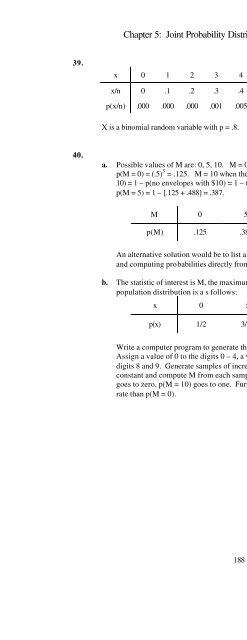
- Page 388: Chapter 5: Joint Probability Distri
- Page 392: Chapter 5: Joint Probability Distri
- Page 396: Chapter 5: Joint Probability Distri
- Page 400: Chapter 5: Joint Probability Distri
- Page 404: Chapter 5: Joint Probability Distri
- Page 408: Chapter 5: Joint Probability Distri
- Page 412: Chapter 6: Point Estimation3.a. We
- Page 416: Chapter 6: Point Estimation9.a. E(
- Page 420: Chapter 6: Point Estimation16.a. E
- Page 424: Chapter 6: Point Estimation21.⎛ 1
- Page 428:
Chapter 6: Point Estimation27.a. f
- Page 432:
Chapter 6: Point Estimation32. spa.
- Page 436:
Chapter 6: Point Estimation38.a. Th
- Page 440:
Chapter 7: Statistical Intervals Ba
- Page 444:
Chapter 7: Statistical Intervals Ba
- Page 448:
Chapter 7: Statistical Intervals Ba
- Page 452:
Chapter 7: Statistical Intervals Ba
- Page 456:
Chapter 7: Statistical Intervals Ba
- Page 460:
Chapter 7: Statistical Intervals Ba
- Page 464:
Chapter 7: Statistical Intervals Ba
- Page 468:
Chapter 7: Statistical Intervals Ba
- Page 472:
Chapter 7: Statistical Intervals Ba
- Page 476:
Chapter 8: Tests of Hypotheses Base
- Page 480:
Chapter 8: Tests of Hypotheses Base
- Page 484:
Chapter 8: Tests of Hypotheses Base
- Page 488:
Chapter 8: Tests of Hypotheses Base
- Page 492:
Chapter 8: Tests of Hypotheses Base
- Page 496:
Chapter 8: Tests of Hypotheses Base
- Page 500:
Chapter 8: Tests of Hypotheses Base
- Page 504:
Chapter 8: Tests of Hypotheses Base
- Page 508:
Chapter 8: Tests of Hypotheses Base
- Page 512:
Chapter 8: Tests of Hypotheses Base
- Page 516:
Chapter 8: Tests of Hypotheses Base
- Page 520:
Chapter 8: Tests of Hypotheses Base
- Page 524:
Chapter 9: Inferences Based on Two
- Page 528:
Chapter 9: Inferences Based on Two
- Page 532:
Chapter 9: Inferences Based on Two
- Page 536:
Chapter 9: Inferences Based on Two
- Page 540:
25. We calculate the degrees of fre
- Page 544:
Chapter 9: Inferences Based on Two
- Page 548:
Chapter 9: Inferences Based on Two
- Page 552:
Chapter 9: Inferences Based on Two
- Page 556:
Chapter 9: Inferences Based on Two
- Page 560:
Chapter 9: Inferences Based on Two
- Page 564:
Chapter 9: Inferences Based on Two
- Page 568:
Chapter 9: Inferences Based on Two
- Page 572:
Chapter 9: Inferences Based on Two
- Page 576:
Chapter 9: Inferences Based on Two
- Page 580:
Chapter 9: Inferences Based on Two
- Page 584:
Chapter 9: Inferences Based on Two
- Page 588:
Chapter 9: Inferences Based on Two
- Page 592:
Chapter 10: The Analysis of Varianc
- Page 596:
Chapter 10: The Analysis of Varianc
- Page 600:
Chapter 10: The Analysis of Varianc
- Page 604:
Chapter 10: The Analysis of Varianc
- Page 608:
Chapter 10: The Analysis of Varianc
- Page 612:
Chapter 10: The Analysis of Varianc
- Page 616:
Chapter 10: The Analysis of Varianc
- Page 620:
Chapter 10: The Analysis of Varianc
- Page 624:
Chapter 10: The Analysis of Varianc
- Page 628:
Chapter 11: Multifactor Analysis of
- Page 632:
Chapter 11: Multifactor Analysis of
- Page 636:
Chapter 11: Multifactor Analysis of
- Page 640:
Chapter 11: Multifactor Analysis of
- Page 644:
Chapter 11: Multifactor Analysis of
- Page 648:
Chapter 11: Multifactor Analysis of
- Page 652:
Chapter 11: Multifactor Analysis of
- Page 656:
Chapter 11: Multifactor Analysis of
- Page 660:
Chapter 11: Multifactor Analysis of
- Page 664:
Chapter 11: Multifactor Analysis of
- Page 668:
Chapter 11: Multifactor Analysis of
- Page 672:
Chapter 11: Multifactor Analysis of
- Page 676:
Chapter 11: Multifactor Analysis of
- Page 680:
Chapter 11: Multifactor Analysis of
- Page 684:
Chapter 11: Multifactor Analysis of
- Page 688:
Chapter 11: Multifactor Analysis of
- Page 692:
Chapter 11: Multifactor Analysis of
- Page 696:
Chapter 11: Multifactor Analysis of
- Page 700:
Chapter 11: Multifactor Analysis of
- Page 704:
Chapter 12: Simple Linear Regressio
- Page 708:
Chapter 12: Simple Linear Regressio
- Page 712:
Chapter 12: Simple Linear Regressio
- Page 716:
Chapter 12: Simple Linear Regressio
- Page 720:
Chapter 12: Simple Linear Regressio
- Page 724:
Chapter 12: Simple Linear Regressio
- Page 728:
Chapter 12: Simple Linear Regressio
- Page 732:
Chapter 12: Simple Linear Regressio
- Page 736:
Chapter 12: Simple Linear Regressio
- Page 740:
Chapter 12: Simple Linear Regressio
- Page 744:
Chapter 12: Simple Linear Regressio
- Page 748:
Chapter 12: Simple Linear Regressio
- Page 752:
Chapter 12: Simple Linear Regressio
- Page 756:
Chapter 12: Simple Linear Regressio
- Page 760:
Chapter 12: Simple Linear Regressio
- Page 764:
Chapter 12: Simple Linear Regressio
- Page 768:
Chapter 12: Simple Linear Regressio
- Page 772:
Chapter 12: Simple Linear Regressio
- Page 776:
Chapter 12: Simple Linear Regressio
- Page 780:
Chapter 12: Simple Linear Regressio
- Page 784:
Chapter 12: Simple Linear Regressio
- Page 788:
Chapter 13: Nonlinear and Multiple
- Page 792:
Chapter 13: Nonlinear and Multiple
- Page 796:
Chapter 13: Nonlinear and Multiple
- Page 800:
Chapter 13: Nonlinear and Multiple
- Page 804:
Chapter 13: Nonlinear and Multiple
- Page 808:
Chapter 13: Nonlinear and Multiple
- Page 812:
Chapter 13: Nonlinear and Multiple
- Page 816:
Chapter 13: Nonlinear and Multiple
- Page 820:
Chapter 13: Nonlinear and Multiple
- Page 824:
Chapter 13: Nonlinear and Multiple
- Page 828:
Chapter 13: Nonlinear and Multiple
- Page 832:
Chapter 13: Nonlinear and Multiple
- Page 836:
Chapter 13: Nonlinear and Multiple
- Page 840:
Chapter 13: Nonlinear and Multiple
- Page 844:
Chapter 13: Nonlinear and Multiple
- Page 848:
Chapter 13: Nonlinear and Multiple
- Page 852:
Chapter 13: Nonlinear and Multiple
- Page 856:
Chapter 13: Nonlinear and Multiple
- Page 860:
Chapter 13: Nonlinear and Multiple
- Page 864:
Chapter 13: Nonlinear and Multiple
- Page 868:
Chapter 13: Nonlinear and Multiple
- Page 872:
Chapter 13: Nonlinear and Multiple
- Page 876:
Chapter 13: Nonlinear and Multiple
- Page 880:
Chapter 14: The Analysis of Categor
- Page 884:
Chapter 14: The Analysis of Categor
- Page 888:
Chapter 14: The Analysis of Categor
- Page 892:
Chapter 14: The Analysis of Categor
- Page 896:
Chapter 14: The Analysis of Categor
- Page 900:
Chapter 14: The Analysis of Categor
- Page 904:
Chapter 14: The Analysis of Categor
- Page 908:
Chapter 14: The Analysis of Categor
- Page 912:
Chapter 14: The Analysis of Categor
- Page 916:
Chapter 15: Distribution-Free Proce
- Page 920:
Chapter 15: Distribution-Free Proce
- Page 924:
Chapter 15: Distribution-Free Proce
- Page 928:
Chapter 15: Distribution-Free Proce
- Page 932:
Chapter 15: Distribution-Free Proce
- Page 936:
Chapter 15: Distribution-Free Proce
- Page 940:
Chapter 16: Quality Control Methods
- Page 944:
Chapter 16: Quality Control Methods
- Page 948:
Chapter 16: Quality Control Methods
- Page 952:
Chapter 16: Quality Control Methods
- Page 956:
Chapter 16: Quality Control Methods
- Page 960:
Chapter 16: Quality Control Methods
- Page 964:
Chapter 16: Quality Control Methods