- Page 2:
Chapter 1: Overview and Descriptive
- Page 6:
Chapter 1: Overview and Descriptive
- Page 10:
Chapter 1: Overview and Descriptive
- Page 16:
Chapter 1: Overview and Descriptive
- Page 20:
Chapter 1: Overview and Descriptive
- Page 24:
Chapter 1: Overview and Descriptive
- Page 28:
Chapter 1: Overview and Descriptive
- Page 32:
Chapter 1: Overview and Descriptive
- Page 36:
Chapter 1: Overview and Descriptive
- Page 40:
Chapter 1: Overview and Descriptive
- Page 44:
Chapter 1: Overview and Descriptive
- Page 48:
Chapter 1: Overview and Descriptive
- Page 52:
Chapter 1: Overview and Descriptive
- Page 56:
Chapter 1: Overview and Descriptive
- Page 62:
Chapter 1: Overview and Descriptive
- Page 66:
Chapter 1: Overview and Descriptive
- Page 70:
Chapter 1: Overview and Descriptive
- Page 74:
Chapter 1: Overview and Descriptive
- Page 78:
Chapter 1: Overview and Descriptive
- Page 82:
Chapter 1: Overview and Descriptive
- Page 86:
Chapter 1: Overview and Descriptive
- Page 90:
Chapter 1: Overview and Descriptive
- Page 94:
CHAPTER 2Section 2.11.a. S = { 1324
- Page 98:
Chapter 2: Probability5.a.OutcomeNu
- Page 102:
Chapter 2: Probability8.a. A 1 ∪
- Page 106:
Chapter 2: Probability9.a. In the d
- Page 110:
Chapter 2: Probabilityf. either (ne
- Page 114:
Chapter 2: Probability17.a. The pro
- Page 118:
Chapter 2: Probability24. Since A i
- Page 122:
Chapter 2: ProbabilitySection 2.329
- Page 126:
Chapter 2: Probability34.⎛20⎞
- Page 130:
Chapter 2: Probabilityd. To examine
- Page 134:
Chapter 2: Probability42. Seats:2
- Page 138:
Chapter 2: Probability47.P(A ∩ B)
- Page 142:
Chapter 2: ProbabilityP(M ∩ SS
- Page 146:
Chapter 2: Probabilityc. P(all H’
- Page 150:
Chapter 2: Probability61. P(0 def i
- Page 154:
Chapter 2: Probability63.a.b. P(A
- Page 158:
Chapter 2: Probability66. Define ev
- Page 162:
Chapter 2: ProbabilitySection 2.568
- Page 166:
Chapter 2: Probability79.Using the
- Page 170:
Chapter 2: Probabilityd. P(passes i
- Page 174:
Chapter 2: ProbabilitySupplementary
- Page 178:
Chapter 2: Probability93.1a. There
- Page 182:
Chapter 2: Probability101.a. The la
- Page 186:
Chapter 2: Probabilityd. For what v
- Page 190:
CHAPTER 3Section 3.11.S: FFF SFF FS
- Page 194:
Chapter 3: Discrete Random Variable
- Page 198:
Chapter 3: Discrete Random Variable
- Page 202:
Chapter 3: Discrete Random Variable
- Page 206:
Chapter 3: Discrete Random Variable
- Page 210:
Chapter 3: Discrete Random Variable
- Page 214:
Chapter 3: Discrete Random Variable
- Page 218:
Chapter 3: Discrete Random Variable
- Page 222:
Chapter 3: Discrete Random Variable
- Page 226:
Chapter 3: Discrete Random Variable
- Page 230:
Chapter 3: Discrete Random Variable
- Page 234:
Chapter 3: Discrete Random Variable
- Page 238:
Chapter 3: Discrete Random Variable
- Page 242:
Chapter 3: Discrete Random Variable
- Page 246:
Chapter 3: Discrete Random Variable
- Page 250:
Chapter 3: Discrete Random Variable
- Page 254:
Chapter 3: Discrete Random Variable
- Page 258:
CHAPTER 4Section 4.11.1∫ −∞11
- Page 262:
Chapter 4: Continuous Random Variab
- Page 266:
Chapter 4: Continuous Random Variab
- Page 270:
Chapter 4: Continuous Random Variab
- Page 274:
Chapter 4: Continuous Random Variab
- Page 278:
Chapter 4: Continuous Random Variab
- Page 282:
Chapter 4: Continuous Random Variab
- Page 286:
Chapter 4: Continuous Random Variab
- Page 290:
Chapter 4: Continuous Random Variab
- Page 294:
Chapter 4: Continuous Random Variab
- Page 298:
Chapter 4: Continuous Random Variab
- Page 302:
Chapter 4: Continuous Random Variab
- Page 306:
Chapter 4: Continuous Random Variab
- Page 310:
Chapter 4: Continuous Random Variab
- Page 314:
Chapter 4: Continuous Random Variab
- Page 318:
Chapter 4: Continuous Random Variab
- Page 322:
Chapter 4: Continuous Random Variab
- Page 326:
Chapter 4: Continuous Random Variab
- Page 330:
Chapter 4: Continuous Random Variab
- Page 334:
Chapter 4: Continuous Random Variab
- Page 338:
Chapter 4: Continuous Random Variab
- Page 342:
Chapter 4: Continuous Random Variab
- Page 346:
Chapter 4: Continuous Random Variab
- Page 350:
CHAPTER 5Section 5.11.a. P(X = 1, Y
- Page 354:
Chapter 5: Joint Probability Distri
- Page 358:
Chapter 5: Joint Probability Distri
- Page 362:
Chapter 5: Joint Probability Distri
- Page 366:
Chapter 5: Joint Probability Distri
- Page 370:
Chapter 5: Joint Probability Distri
- Page 374:
Chapter 5: Joint Probability Distri
- Page 378:
Chapter 5: Joint Probability Distri
- Page 382:
Chapter 5: Joint Probability Distri
- Page 386:
Chapter 5: Joint Probability Distri
- Page 390:
Chapter 5: Joint Probability Distri
- Page 394:
Chapter 5: Joint Probability Distri
- Page 398:
Chapter 5: Joint Probability Distri
- Page 402:
Chapter 5: Joint Probability Distri
- Page 406:
Chapter 5: Joint Probability Distri
- Page 410:
CHAPTER 6Section 6.11.a. We use the
- Page 414:
Chapter 6: Point Estimation6.a. Let
- Page 418:
Chapter 6: Point Estimation(.635)(.
- Page 422:
Chapter 6: Point Estimation19.λ ,
- Page 426:
Chapter 6: Point Estimation23. For
- Page 430:
Chapter 6: Point Estimation29.a. Th
- Page 434:
Chapter 6: Point Estimation35.xi+ x
- Page 438:
CHAPTER 7Section 7.11.z implies tha
- Page 442:
Chapter 7: Statistical Intervals Ba
- Page 446:
Chapter 7: Statistical Intervals Ba
- Page 450:
Chapter 7: Statistical Intervals Ba
- Page 454:
Chapter 7: Statistical Intervals Ba
- Page 458:
Chapter 7: Statistical Intervals Ba
- Page 462:
Chapter 7: Statistical Intervals Ba
- Page 466:
Chapter 7: Statistical Intervals Ba
- Page 470:
Chapter 7: Statistical Intervals Ba
- Page 474:
CHAPTER 8Section 8.11.a. Yes. It is
- Page 478:
Chapter 8: Tests of Hypotheses Base
- Page 482:
Chapter 8: Tests of Hypotheses Base
- Page 486:
Chapter 8: Tests of Hypotheses Base
- Page 490:
Chapter 8: Tests of Hypotheses Base
- Page 494:
Chapter 8: Tests of Hypotheses Base
- Page 498:
Chapter 8: Tests of Hypotheses Base
- Page 502:
Chapter 8: Tests of Hypotheses Base
- Page 506:
Chapter 8: Tests of Hypotheses Base
- Page 510:
Chapter 8: Tests of Hypotheses Base
- Page 514:
Chapter 8: Tests of Hypotheses Base
- Page 518:
Chapter 8: Tests of Hypotheses Base
- Page 522:
CHAPTER 9Section 9.11.a. E ( X −
- Page 526:
Chapter 9: Inferences Based on Two
- Page 530:
Chapter 9: Inferences Based on Two
- Page 534:
Chapter 9: Inferences Based on Two
- Page 538:
Chapter 9: Inferences Based on Two
- Page 542:
Chapter 9: Inferences Based on Two
- Page 546:
Chapter 9: Inferences Based on Two
- Page 550:
Chapter 9: Inferences Based on Two
- Page 554:
Chapter 9: Inferences Based on Two
- Page 558:
50. Let = . 05Chapter 9: Inferences
- Page 562:
Chapter 9: Inferences Based on Two
- Page 566:
Chapter 9: Inferences Based on Two
- Page 570:
Chapter 9: Inferences Based on Two
- Page 574:
Chapter 9: Inferences Based on Two
- Page 578:
78. Let µ1denote the true average
- Page 582:
Chapter 9: Inferences Based on Two
- Page 586:
Chapter 9: Inferences Based on Two
- Page 590:
CHAPTER 10Section 10.11.a. H o will
- Page 594:
Chapter 10: The Analysis of Varianc
- Page 598:
Chapter 10: The Analysis of Varianc
- Page 602:
Chapter 10: The Analysis of Varianc
- Page 606:
Chapter 10: The Analysis of Varianc
- Page 610:
Chapter 10: The Analysis of Varianc
- Page 614:
Chapter 10: The Analysis of Varianc
- Page 618:
Chapter 10: The Analysis of Varianc
- Page 622:
Chapter 10: The Analysis of Varianc
- Page 626:
CHAPTER 11Section 11.11.30.659.27.6
- Page 630:
Chapter 11: Multifactor Analysis of
- Page 634:
Chapter 11: Multifactor Analysis of
- Page 638:
Chapter 11: Multifactor Analysis of
- Page 642:
Chapter 11: Multifactor Analysis of
- Page 646:
Chapter 11: Multifactor Analysis of
- Page 650:
Chapter 11: Multifactor Analysis of
- Page 654:
Chapter 11: Multifactor Analysis of
- Page 658:
Chapter 11: Multifactor Analysis of
- Page 662:
Chapter 11: Multifactor Analysis of
- Page 666:
Chapter 11: Multifactor Analysis of
- Page 670:
Chapter 11: Multifactor Analysis of
- Page 674:
Chapter 11: Multifactor Analysis of
- Page 678:
Chapter 11: Multifactor Analysis of
- Page 682:
Chapter 11: Multifactor Analysis of
- Page 686:
Chapter 11: Multifactor Analysis of
- Page 690:
Chapter 11: Multifactor Analysis of
- Page 694:
Chapter 11: Multifactor Analysis of
- Page 698:
Chapter 11: Multifactor Analysis of
- Page 702:
CHAPTER 12Section 12.11.a. Stem and
- Page 706:
Chapter 12: Simple Linear Regressio
- Page 710:
Chapter 12: Simple Linear Regressio
- Page 714:
Chapter 12: Simple Linear Regressio
- Page 718:
Chapter 12: Simple Linear Regressio
- Page 722:
Chapter 12: Simple Linear Regressio
- Page 726:
Chapter 12: Simple Linear Regressio
- Page 730:
Chapter 12: Simple Linear Regressio
- Page 734:
Chapter 12: Simple Linear Regressio
- Page 738:
Chapter 12: Simple Linear Regressio
- Page 742:
Chapter 12: Simple Linear Regressio
- Page 746:
Chapter 12: Simple Linear Regressio
- Page 750:
Chapter 12: Simple Linear Regressio
- Page 754:
Chapter 12: Simple Linear Regressio
- Page 758:
Chapter 12: Simple Linear Regressio
- Page 762:
Chapter 12: Simple Linear Regressio
- Page 766:
Chapter 12: Simple Linear Regressio
- Page 770:
Chapter 12: Simple Linear Regressio
- Page 774: Chapter 12: Simple Linear Regressio
- Page 778: Chapter 12: Simple Linear Regressio
- Page 782: Chapter 12: Simple Linear Regressio
- Page 786: CHAPTER 13Section 13.11.2x and ∑
- Page 790: Chapter 13: Nonlinear and Multiple
- Page 794: Chapter 13: Nonlinear and Multiple
- Page 798: Chapter 13: Nonlinear and Multiple
- Page 802: Chapter 13: Nonlinear and Multiple
- Page 806: Chapter 13: Nonlinear and Multiple
- Page 810: Chapter 13: Nonlinear and Multiple
- Page 814: Chapter 13: Nonlinear and Multiple
- Page 818: Chapter 13: Nonlinear and Multiple
- Page 822: Chapter 13: Nonlinear and Multiple
- Page 828: Chapter 13: Nonlinear and Multiple
- Page 832: Chapter 13: Nonlinear and Multiple
- Page 836: Chapter 13: Nonlinear and Multiple
- Page 840: Chapter 13: Nonlinear and Multiple
- Page 844: Chapter 13: Nonlinear and Multiple
- Page 848: Chapter 13: Nonlinear and Multiple
- Page 852: Chapter 13: Nonlinear and Multiple
- Page 856: Chapter 13: Nonlinear and Multiple
- Page 860: Chapter 13: Nonlinear and Multiple
- Page 864: Chapter 13: Nonlinear and Multiple
- Page 868: Chapter 13: Nonlinear and Multiple
- Page 872: Chapter 13: Nonlinear and Multiple
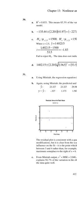
- Page 876:
Chapter 13: Nonlinear and Multiple
- Page 880:
Chapter 14: The Analysis of Categor
- Page 884:
Chapter 14: The Analysis of Categor
- Page 888:
Chapter 14: The Analysis of Categor
- Page 892:
Chapter 14: The Analysis of Categor
- Page 896:
Chapter 14: The Analysis of Categor
- Page 900:
Chapter 14: The Analysis of Categor
- Page 904:
Chapter 14: The Analysis of Categor
- Page 908:
Chapter 14: The Analysis of Categor
- Page 912:
Chapter 14: The Analysis of Categor
- Page 916:
Chapter 15: Distribution-Free Proce
- Page 920:
Chapter 15: Distribution-Free Proce
- Page 924:
Chapter 15: Distribution-Free Proce
- Page 928:
Chapter 15: Distribution-Free Proce
- Page 932:
Chapter 15: Distribution-Free Proce
- Page 936:
Chapter 15: Distribution-Free Proce
- Page 940:
Chapter 16: Quality Control Methods
- Page 944:
Chapter 16: Quality Control Methods
- Page 948:
Chapter 16: Quality Control Methods
- Page 952:
Chapter 16: Quality Control Methods
- Page 956:
Chapter 16: Quality Control Methods
- Page 960:
Chapter 16: Quality Control Methods
- Page 964:
Chapter 16: Quality Control Methods