Huygens Professional User Guide

Huygens ProfessionalUser GuideS IScientific Volume Imaging

S IHuygens ProfessionalUser GuideVersion 2.10Scientific Volume Imaging B.V.Laapersveld 631213 VB HilversumP.O. box 6151200 AP HilversumThe Netherlands

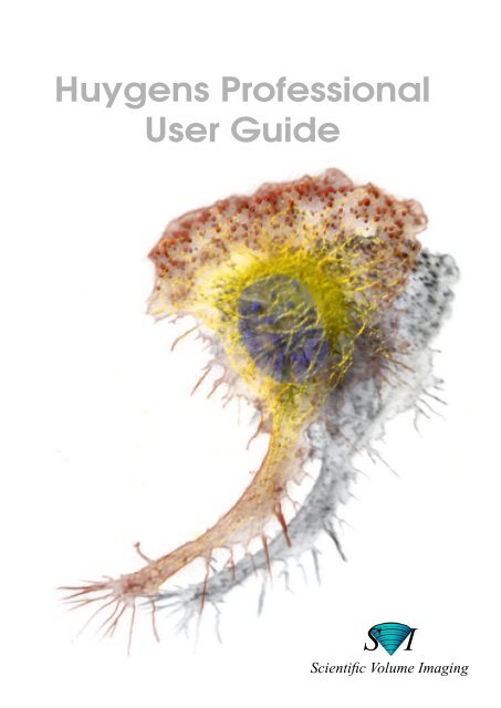
Copyright © 1997-2006 by Scientific Volume Imaging B.V.,Laapersveld 63, 1213 VB HilversumP.O. box 615,1200 AP Hilversum,The NetherlandsAll rights reservedCover illustration:Macrophage recorded by Dr. James Evans, Whitehead Institute, MIT, Boston MA,USA, using wide field microscopy.At the right the same dataset: Macrophage fluorescently stained for tubulin (yellow/green), actin (red) and the nucleus (DAPI, blue). Left part: original data; right part:as deconvolved with the classical Maximum Liklihood Etimation method (MLE).The image was visualized using FluVR. FluVR is the advanced Simulated FluorescenceProcess (SFP) volume rendering package from Scientific Volume Imaging.doc proUserGuide 2.6.02

CHAPTER 1 Introduction 3contents 3What is Huygens Professional? 3Image deconvolution functions 3Basic image processing capabilities 3Core image processing functions 4Reporting & display operations 4Image file I/O 4Analysis functions 4Visualization 4Installation and system requirements 4Installing the Huygens Professional. 4Installing the software 4Obtaining a license key 5Installing the license key 5System requirements 5Memory requirements 5Irix 5Linux 5Addresses and URLs 6Where can we be reached? 6Support and FAQ 6Where can I find more about Silicon Graphics? 6IBM Life Sciences 6CHAPTER 2 Getting Started 7Deconvolving my first image 7Searching the SVI Knowledge Base 7Step 1: Start Huygens Pro 7Step 2: Load an image 8Step 3: Inspect your image. 8bleaching correction 11Step 4: Generate a Point Spread Function (PSF) 12Step 5: Estimate the average background in the image. 12Step 6: Estimate the Signal to Noise ratio (SN ratio) 13Step 7: Perform a deconvolution run, applying the MLE (Maximum Likelihood Estimation) method.13Step 8: Saving your image 14The easy way 14Quick and easy deconvolution 14MLE-time 14MLE-time Buttons and input fields 15Padding and widefield images 17Why is automatic deconvolution essential? 17CHAPTER 3 Establishing image parameters 19Image size 19Brick wise processing 19Signal to Noise Ratio (SNR) 20Blacklevel 20Sampling densities 21Data acquisition pitfalls 21Refractive index mismatch 21Clipping 22Undersampling 22The Huygens Professional User Guide 1

2 The Huygens Professional User GuideDo not undersample to limit photodamage 22Bleaching 22Illumination instability 22Mechanical instability 22Thermal effects 23Internal reflection 23Computing the backprojected pinhole radius 23Airy disk as unit for the backprojected pinhole 23Converting from integer parameter 23Airy disk as unit for the backprojected radius of a square pinhole 24Computing the backprojected pinhole distance in Nipkow spinning disks 24Pinhole radius tables 24Leica confocal microscopes 24Zeiss confocal microscopes 25Olympus confocal microscopes 25Biorad confocal microscopes 26A supplied calibration curve 26Questions 26What does the quality factor mean while running Huygens? 26Can I deconvolve a Tiff series? 27Tiff file series naming convention 27Can I deconvolve a single plane widefield image? 28Can I deconvolve a single Tiff image? 28

CHAPTER 1IntroductionThis guide is useful to the beginner in deconvolution and to the expert that startsusing the Huygens Professional toolkit.For the expert we recommend also to study the Huygens Reference Manual.contentsIn chapter 1 we explain the installationIn chapter 2 you deconvolve your first imageIn chapter 3 we help you determining some important parameters and give you hints for basicimage data-acquisitionWhat is Huygens Professional?Huygens professional is an image processing software package tailored for deconvolution ofmicroscopic images. It enables you to deconvolve a wide variety of images ranging from 2Dwidefield (WF) images to 4D multi-channel two-photon confocal images or from Scanningdisk confocal microscopes. Also people who use experimental set-ups like 4p-microscopesmay benefit from the software. The Huygens Professional toolbox contains the following features:Image deconvolutionfunctionsBasic image processingcapabilities• Accelerated Maximum Likelihood Estimation restoration algorithm optimized for low light levelimages• Iterative Constrained Tikhonov-Miller restoration algorithm• Quick Tikhonov-Miller and Quick MLE restoration algorithms• Point Spread Function (PSF) measurement tool box to derive a microscopic PSF from finite sizedmicro bead images, containing:• Automatic alignment and averaging procedure to combine the signal from different micro beads in oneor more images• PSF reconstruction tool to correct for the finite size of micro beads• Generates a theoretical Point Spread Function for widefield, confocal and two-photon microscopesbased on electromagnetic diffraction theory• Automatic bleaching correction of 3D and 4D widefield images and 4D confocal and multi-photonimages• Z-drift corrector tool for timeseries that enables you to correct for movement in the Z (axial) directionthat could have been occurred for instance by thermal drift of the microscope table.• Capability to handle multiple images• Time series support• Multi parameter (multi channel) image elements (stacked or packed)• Basic data types: unsigned byte, 16 bit signed integer, 32 bit float, 2 x 32 bit complex• Per image undo/redo capabilities• Scripting and batch processing environment based on Tcl (Tool Command Language)The Huygens Professional User Guide 3

Installation and system requirementsCore image processingfunctionsReporting & displayoperationsImage file I/OAnalysis functionsVisualization• Create, destroy, copy, copy block, convert, split, join, zoom, rotate, iso-sample, shift, replicate image• Add/remove border, shift to sub-pixel accuracy, mirror image, swap image octants• Arithmetic operations on two image operands, one image operand and a scalar, mathematical functionson one image operand, soft clipping & thresholding• 4D Gaussian filter of arbitrary widths, 4D Laplacian filter• Generate solid and hollow bandlimited spheres, generate Poisson and Gaussian noise• Real and complex 4D Fast Fourier transforms• Image statistics• Report sampling density with respect to Nyquist rate• Image histograms of images with up to three channels• Plots of Energy Flux as function of time and axial position• Reads ICS, Imaris® classic, numbered series TIFF, Zeiss Lsm, Metamorph STK, Biorad pic, Olympus’Fluoview’, Leica files and Delta Vision IMSubs (r3d), IPLab Tiff.• Writes ICS, Imaris® classic, Biorad pic, TIFF (Leica style and classic numbered series TIFF).• 4D read support: ICS, numbered ‘stk’, numbered Leica-TIFF, numbered TIFF• Export to FluVR, the volume renderer based on spectral fluorescence• Export to Imaris®• Threshold and label 3D image• Analyze labelled objects: compute centre of mass, volume and integrated intensity• Estimate background• Measure distance• Compute image ratio• Compute colocalization coefficients• Compute the co-occurrence matrix of an image• Thumbnail images• Multiple Expand viewers on one or more images. Each Expand viewer is able to• Show x-y, x-z or y-z slices for selectable points in time while optimizing contrast on a global or perplanebasis• Show Sum or MIP projection, animate projections of time series• Display single channel images in False or True color; multi channel images in True color• Report individual pixel/voxel positions and values• Swing through planes or time• Slicing positions in expand viewers can be dynamically linked for easy image comparisonInstallation and system requirementsInstalling the Huygens Professional.Installing the softwareLinuxThe Huygens professional Linux distribution is a so-called ‘rpm’ file.Example: Your rpm file is called: huygens-2.9.1-p0.rpmTo install this file you open a shell, go to the directory where this file is located, become superuserand type:rpm -Uvh huygens-2.9.1-p0.rpmnote: capital ‘U’ and space between ‘rpm’ and ‘-’.4 The Huygens Professional User Guide

Installation and system requirementsAfter installing the software type huygens2 in a shell to start the software. A directory/usr/local/svi will be created; the executables will be installed in /usr/local/binIrixCurrently the Irix distribution is a single ‘tardist’ file containing various components. Bydefault all components are installed. Become superuser and type:swmgr -f huygens-2.9.1-p0.tardistPress ‘Start’ in the Software Manager window.A directory /usr/local/svi will be created; the executables will be installed in /usr/local/bin and/usr/sbin.Obtaining a licensekeyTo run the software beyond the freeware functionality you will need a license key. A temporarylicense key can be obtained by sending SVI a reply on the email that was sent to you when youdownloaded the software.Please answer the questions in the email and paste your computer’s system ID at the correctplace. Your computer’s system ID can be read in the Menu item Help>Product information.Once we have received the system ID together with the information from your reply and theoriginal email, we will generate a personalized license for your system. This license will onlywork on that specific computer.Installing the licensekeyThe installation created a file huygensLicense in the directory /usr/local/svi. Become root andadd the license string on a separate line in the file.System requirementsMemory requirementsIrixLinuxRecommended RAM memory: 512 MB or larger.All SGI equipment running Irix 6.5 running Irix 6.5 on a MIPS R5000 processor or higher. OnOctane or higher systems automatically a 64bit multiprocessing executable is installed. Thisallows the software to access more than 4GB of RAM and to distribute the computational workover many processors.• All SVI packages on Irix require the SCSL mathematical library. This is distributed along with Irix; anup to date version can be downloaded from the SGI web site.Linux: RedHat and SuSE distributions. Since Linux versions evolve rapidly best consult SVI’swww.svi.nl web page to see which Linux distributions are currently supported.A standard ethernet card is required to provide your computer with a system ID.• Processor: Pentium III or IV (Intel) or Athlon (AMD).• Graphics card: any fairly modern card will do.The Huygens Professional User Guide 5

Installation and system requirementsAddresses and URLsWhere can we bereached?Scientific Volume Imaging B.V.Laapersveld 631213 VB HilversumThe NetherlandsYou can call us directly by phone:++31 35 6421626,or fax us at: ++31 35 6837971,or email us at: info@svi.nlhttp://www.svi.nlDistributorsA list of distributors can be found on our web site:http://www.svi.nl/distributorsSupport and FAQPlease visit the following web site for support issues and to consult the FAQ:http://support.svi.nlOn this web site you’ll also find a form to submit questions to SVI’s support team.Where can I find moreabout Silicon Graphics?IBM Life SciencesPlease visit the SGI web site:http://www.sgi.comThere you can find addresses of sales and support offices which exist in many countries.http://www-1.ibm.com/industries/lifesciences/6 The Huygens Professional User Guide

CHAPTER 2Getting StartedThis chapter will help you to get through the basic procedures in deconvolving animage.Deconvolving my first imageSearching the SVIKnowledge BaseStep 1: Start HuygensProIt’s good to know that an extensive support base is available where you may find answers toquestions that come to front while reading this document. FAQ’s are available for many itemssuch as deconvolution and general microscopy, installation, memory management, visualization,file formats, platforms and reported bugs.:http://support.svi.nl/Starting Huygens Pro- IRIX: You may start the Huygens program by clicking the ‘Icon Catalog’ on your Irix desktop.- LINUX: Via the KDE application menu.- LINUX / IRIX: By opening a shell and typing ‘huygens2’. It is a good idea first to go to thedirectory where your images are stored, using the command ‘cd’.Figure 1. Starting Huygens Pro. If you type an ampersand (&) after thecommand the prompt (>) will return.The huygens2 command starts the program that comes up with the Main Window with 4black thumbnail images (see Figure 2).The Huygens Professional User Guide 7

Deconvolving my first imageFigure 2. The Main Window with empty thumbnail images loaded by default.Thumbnail imagesStep 2: Load an imageThe Main Window is initially loaded with 4 black thumbnail images, images that are alreadyprepared for you, but where all image data are zero’s. One of the images is called ‘psf’ whichwill be used in the deconvolution steps as you will learn soon.Loading your imageFirst you have to load an image. Select ‘Open’ from the File menu in the Main Window andfind the file to be processed.In the distribution you will find the demo image faba32 (the file pair faba32.ids and faba32.ics,where faba32.ids is the file containing the raw data and faba32.ics is a header file, containingall microscope parameters). Click on one of these, no matter which one.You may combine steps 1 and 2: starting Huygens and loading images using a single commandline:huygens2 faba32.ics dama.ids&This command appends the images faba32 and dama to the Main window.If you have Tiff slices to be processed please read “Tiff file series naming convention” onpage 27 for the naming convention in order to be able to read a multi-dimensional image as awhole.Step 3: Inspect yourimage.Inspect your image.• Use the slicerExpand viewer Open the Expand viewer by pressing the Arrow-up button from the thumbnail offaba32. The Expand viewer is intended as a general purpose image inspection tool. It iscomposed of a menu bar and a tabbed deck consisting of a Projection page, a Slicer Page8 The Huygens Professional User Guide

Deconvolving my first imageand a Parameters page. You can open as many Expand viewers as you like, on the sameimage or on different images.image is not a timeseries.‘t’-slicing is notavailable.Figure 3. Two Expand Viewers opened from the same image. Left theSlicer Tab is selected, right the Projection Tab.With the Viewer’s Slicer you can scan through the slices (in different directions). Since thisexample image is not a time series, the time (t) select box is greyed.Microscopic parameters • Verify the microscopic parameters (needed for the generationof a PSF) like Numerical Aperture, Microscope type, samplesize, etc. by selecting the Parameters Tab from the Expandviewer (see Figure 3).Did you use the correct Sampling size? To find out, selectfaba32 in the Main window, by clicking on the image (thename is displayed in blue, when selected!). Now select‘Nyquist rate’ from the Edit menu and you will be informed.We see that the image is fairly good sampled in the x and y directions since the nyquist rateis near to the value of one. However, the z (the x-y slices) is undersampled (the samplingwas too course). Advised is to sample in the z-direction with a distance of 166 nm or less.Conclusion: if the Nyquist tool leaves you with values smaller then one you have undersampledyour image. Tough luck for you now, but hopefully future recordings may benefitfrom this information.(Super sampling of an image is not a problem, although your dataset becomes unnecessarilylarge without providing extra information).For now we continue with the z-undersampled demo image.The Huygens Professional User Guide 9

Deconvolving my first imageHistogram • The image histogramSelect the image in the Main Window and selectImage histogram from the Edit menu. An image histogramis created as a thumbnail image namedfaba32:histo. You may use the Expand viewer for abetter view. The histogram enables you to inspectthe quality of the image visually. The one inFigure 4 is of reasonable quality: No sharp peaks atthe extreme sites of the histogram image indicatingclipping. An example of a clipped image is shownbelow.Not also that the black space at the left hand of thehistogram. It signifies an electronic mismatch in therecording of the image. See “Blacklevel” onpage 20.A clipped image example, see Figure 5.If you see a narrow peak at the left hand side of thehistogram this signifies ‘clipping’. It occurs whennegative input signals are mapped to zero’s by theCCD camera. See also “Clipping” on page 22.If a peak is visible at the extreme right hand side ofthe histogram it indicates saturation. Saturation is atype of clipping caused by raising the laser intensityabove the maximum pixel value available on yourmicroscope. Usually, all values above the maximumvalue are replaced by the maximum value. On rareoccasions they are replaced by zeroes. Clipping willhave a negative effect on the results of deconvolution,especially with WF imagesFigure 4. The image histogramfrom the exampleFigure 5. The image histogramfrom a clipped image. A spike isseen at the left hand site.Operations windowIn the former steps all operations were performed without any operation parameters (functionsapplicable on a particular image). For example if one wants to know the image statistics noextra information is needed but the name of the image. All these types of operations are accessiblefrom the main Window. Most operations, however, need extra input data. For exampleadding some constant value to an image. This can be done in the Operations WindowSince in the next steps all image processing operations need one or more parameters you haveto work with the Operations window. You open an Operations window on an image by clickingon the small button labelled O in the images’ Thumbnail component.10 The Huygens Professional User Guide

Deconvolving my first imageSubsequently you select an operation from the Menu bar or from the Quick access buttons. TheMenu barQuick access buttonsFigure 6. The Operation window with the PSF buttonpressed.left side of the operation window is similar to the Expand viewer. At the right side you will findthe parameter entry area. By editing the parameters you control the way the function operates.To execute the operation, press the RUN button.bleaching correctionIntermezzo: check for bleaching correctionRemember, we were inspecting our image.This extra check is given here for the sake of completenessfor those using this schematic approachfor widefield images or confocal time series. Select‘Plot Flux’ from the ‘Analysis’ menu in the Operationwindow. A typical example is shown inFigure 7. The Demo image is a regular confocalimage: bleaching correction test makes no sensehere!• Extra check to see if bleaching correction isneeded in widefield images or confocal timeSeries. While recording widefield images orconfocal time series strong bleaching mayoccur.Figure 7. A typical example of ableached widefield image. Use the‘Plot Flux’ tool from the Analysismenu available in the Operationwindow.The Huygens Professional User Guide 11

Deconvolving my first imageStep 4: Generate aPoint Spread Function(PSF)Step 5: Estimate theaverage background inthe image.Figure 8. The PSF in x-z view,using ‘compress’ contrastmode. ‘Compressed contrast’highlights the low intensityvalues showing the typicaldiabolo shape in lateral view.The PSF is the way in which a point of your originalobject is visualized in the image you’ve loaded in step 1.Often this point is no longer a point but blurred andspread out. The aim of the PSF is to calculate the measureof blurring in the x,y,z axis. In the final step ofdeconvolution this PSF is used to come to a (in contradictionto the so-called ‘blind deconvolution) measureddeconvolution. A PSF can be obtained either by recordingsmall beads with known bead diameter (180 nmbeads work fine) and reconstructing a PSF from thebead image or by calculating a theoretical PSF from theinformation about your microscope settings, see“Microscopic parameters” on page 9. Huygens Pro hasmany tools to handle the first method but these arebeyond the scope of this demo. For this first image demowe generate a theoretical one.A theoretical PSF can be generated by clicking the buttonPSF from the Operation Window. This tool computesa Point Spread function from the microscopicparameters. You need not change by now the parameters.By default the psf-image will be displayed in the destination ‘psf’, which is still empty,but any available image can be selected. Press the Run button located in the right down corner.In thumbnail ‘psf’ you may select the Expand viewer to see the Point Spread Function indetail. (Figure 8)In this stage the average background in a volume image is estimated. The average backgroundis thought to correspond with the noise-free equivalent of the measured (noisy) image. It isdetermined by searching the image first for a region with low values. Subsequently the backgroundis determined by searching this region for the planar region with radius r which has thelowest value. It is important for the search strategy that the microscopic parameters of theimage are correct, in especially the sampling distance and the microscope type.The average background estimation is invoked by Estimate background from the Analysismenu in the Operation window. The following choices are possible here:• LOWEST VALUE (Default): The image is searched for a 3D region with the lowest averagevalue. The axial size of the region is around 0.3 micron; the lateral size is controlled by theradius parameter which is set to 0.5 micron by default.• IN/NEAR OBJECT: The neighborhood around the voxel with the highest value is searchedfor a planar region with the lowest average value. The size of the region is controlled by theradius parameter.• WIDEFIELD: First the image is searched for a 3D region with the lowest values to ensurethat the region with the least amount of blur contributions is found. Subsequently the backgroundis determined by searching this region for the planar region with radius r that hasthe lowest value.We are looking for the background outside the object, in a confocal image, therefore we choosefor the default ‘Lowest value’ setting. Again press the Run button. The result is displayed inthe Main window’s Task reports. It is one of the values that should be known in the next step.12 The Huygens Professional User Guide

Deconvolving my first imageStep 6: Estimate theSignal to Noise ratio(SN ratio)The Signal to Noise ratio (SN) is a numbernot always easy to estimate. The easiestway to obtain some figure is to look atthe textures of bright areas in your objectimage. In the figure at left you see examplesof such textures obtained from originallythe same object image to whichvarious levels of poisson noise wereadded.SN = 30SN = 15 SN = 5Figure 9. Images with different generatednoise levelsStep 7: Perform adeconvolution run,applying the MLE(Maximum LikelihoodEstimation)method.Applying the deconvolution processYou can choose between various deconvolution methods. Only in some special cases youshould use the ICTM (Iterative Constraint Tikhonov-Miller) method as explained in the referencemanual. While selecting the MLE-button you‘ll see the following parameter valueswhich can be adapted:Figure 10. The Operations window with the MLE button pressed.• Number of iterations: this depends on the initial quality of your image.(e.g. 20 to 40)• Signal to noise ratio: You have to make an estimation of the Signal to noise (SN) value fromyour recorded image. Inspect your image and decide if your image is noisy (S/N < 10), hasmoderate noise (10-20) or is a low-noise image (S/N> 20). See examples of noisy images inFigure 9• Background: This value was calculated in step 5. Copy the value from the Tasks reports(Main window) into the field.• Threshold quality: This number gives the maximum difference between the subsequentiterations. If one chooses a high number (e.g. 0.1) the deconvolution may stop before theindicated number of iterations has been completed as the threshold value has been reachedbeforehand. The smaller the threshold and the larger the number of iterations the higher thequality of deconvolution.• Other parameters like bleaching correction and padding mode are best kept in their defaultmodes.The Huygens Professional User Guide 13

The easy way• Press the Run button! You will end up witha restored image ‘c’ in the Main window.After inspecting the result in the Expandviewer you may want to perform anotherdeconvolution run. Maybe you also wish tochange one or more parameters. After pressingthe Run button again you will be asked, in thecase the output image destination is notchanged, if you like to do a completely newrun (the destination image is zero-ed before)or one on top of the first run.Figure 11. The Main Window with adeconvolved image ’c’.Step 8: Saving yourimageIf you are done and wish to save the result go to the Main window and select the restored image(c) by clicking its thumbnail (the name is in blue when selected!). From the File menu youselect the Save as ICS (International Cytometry Standard file format) or the Save as ... for someother file formats.The easy wayIn the former part you learned some basic procedures for the deconvolution process and familiarizedyou with some User interface components. This approach is in two minds about educationand demoing functionality. Deconvolution can be done easier.Quick and easy deconvolutionFollowing the steps from the former example you have learned that a PSF is essential to deconvolution.You restored your data using a PSF-image located in ’psf’, which is either an existingmeasured PSF obtained from bead images or a theoretical PSF generated from the parametersof the parent image. You have generated a theoretical PSF and you may have noticed that youneed not inspect nor manipulate this image. And also that the background estimation tool generateda number that need to be copied by hand in the MLE deconvolution process. Since thereis no basic user interaction these steps can be automated. This is done in the MLE-time or theQMLE tools available (Buttons) from the Operation window.MLE-timeThe MLE-time tool is the most versatile deconvolution tool accessible from the Huygens Pro.It can be used for any type of data, no matter whether this is a 2D widefield image or a confocaltime series. If a theoretical PSF is good enough to get by, you can skip generating one yourselfas it is done on the fly.• There is just one thing to wait for, no extra button presses.• Especially while using large images that are processed brick-wise the PSF is preventedfrom being unnecessary large, it adapts its size to the brick size.• In case of a multi channel image the PSF is generated for one channel at the time insteadfor all at once14 The Huygens Professional User Guide

The easy way• The PSF image is thrown away as early as possible, at least before the iterations begin.Downside is that an automatically generated PSF is never re-used.Note: The MLE-time is basically the same deconvolution tool as used in the Huygens Essential.Therefore there is no difference between the theoretical PSF’s as generated by HuygensPro and the Huygens Essential.We recommend to use the MLE-time tool for all your deconvolutionwork. Only in special occasions you have recourse to othertools as is explained in ’Which deconvolution method should youuse?’ from the Huygens Recipes.From step 4 we repeat the deconvolution process using the ‘MLE-time’.Proceed as follows: either Exit Huygens Pro by ‘Exit’ from the File menu in the Main windowand start a Huygens Pro from scratch and open faba32 again, or continue the session after havingcleaned images ‘psf’ and ‘c’. (click on the thumbnail image, and select ‘Zero image’ fromthe edit menu, or use the shortcut ‘ALT+Z’).Open an Operation Window from the original image (faba32). Now press Button MLE-timeand you see the display as shown in Figure 12.Figure 12. The Operations window with the MLE-time button pressed.Use all default values except the ‘Signal/Noise per channel’. We will use the value ‘10’ hereinstead of the default value ‘20’. In the input field you see 4 numbers as prepared for a 4 channelimages. We are dealing with a single channel image here therefore only the first numbershould be changed to ‘10’. If you do so and press ‘Run’, your restored image will be made as‘c’.MLE-time Buttonsand input fieldsSince the MLE-time is the key deconvolution tool we will explain the MLE-time relatedparameters one by one.• PSF (if available)Here you may select from the list of all opened images that particular image that is used asthe PSF image. This can be either a measured PSF or an earlier generated PSF (using the‘PSF’ button from the Operations window). If you don’t use a measured PSF we recommendto select the empty image ‘psf’. In this case a PSF is ‘not available’ and the softwaregenerates PSF’s on the fly.The Huygens Professional User Guide 15

The easy way• Destination of the Output imageSelect an image into which the result will be stored.• Signal/Noise per channelHere you may give the S/N for the separate channels.• Max. iterationsAbsolute stopping criterion. See also ‘Quality change threshold’ below.Deconvolution as it is done in the Huygens compute engine hinges around the idea of findingthe best possible estimate of the object that is imaged by the microscope. To assess thequality of an estimate, the deconvolution algorithm computes the image of each estimate asit would appear in the microscope and compares it with the measured image. From the differencea quality factor is computed. The difference is also used to compute a correctionfactor to modify the estimate in such a way that the corrected estimate will yield a betterquality factor. This is an iterative process that should have a stopping criterion. If the processhas not yet been stopped by the ‘Quality change threshold’ it will be explicitly stoppedby the number of Maximum iterations.• Search for backgroundSeveral choices can be made: AUTO, MANUAL, LOWEST VALUE, IN/NEAR OBJECT OR WIDEFIELD MODE.In manual mode the background value should be specified in the Estimated backgroundinput widget.• Backgr. per ch. (absolute or %)This parameter should be set to the estimated mean background in the measured image.When restoring time series the background is likely to vary from frame to frame. The timeenableddeconvolution tools can therefore make a survey of the background in all framesand channels. The way this survey is carried out is determined by the ‘Search for background’option.Since the backgrounds established by the survey are conservative values (unless In/nearobject is selected) they can be increased by a percentage. For instance 10% means all backgroundestimates are increased by 10%. Negative percentages are also valid.If the ‘search for background’ is in Manual-mode the number is an absolute value and willbe applied ‘as is’ to all frames. This value will be subtracted from all images in all frames.• Bleaching correctionThe bleaching correction can be ‘If possible’ or ‘Off’. In the If possible mode the softwarecorrects for bleaching automatically. The correction is possible for 3D and 4D widefieldimages or 4D confocal images. For 3D confocal images automatic bleaching correction isnot possible.• Threshold for quality factor increase (%)This is the primary stopping criterion. After each iteration a quality factor is computedfrom the new estimate. This factor is based on the so-called I-divergence or cross-entropymeasure of the original image and the imaged estimate. You can set a stop criterion in theform of a threshold on the quality increase. When the quality drops below the threshold fora few iterations in succession, iterations are stopped.When the quality is decreasing, iterations are stopped immediately. This occurs with poorquality PSFs.When set to 0 the stop criterion is inactive and even in the case of decreasing quality, iterationswill continue.• Iteration modeThis allows the selection of a Fast mode or a High Quality mode. In Fast mode the iterationsare more effective at the cost of a marginal increase of computing time per iterationand the addition of one extra (hidden) temporarily image.• Padding modePadding means that a border will be added around an image which is not only needed fortrivial things like creating extra space to be able to rotate an image without having its cornerscutted off, but also to prevent ‘wrap around’ effects caused by the use of discrete FourierTransforms (DFT) which interprets the image as periodic, i.e. the image is continued onall sides by exact copies of itself. Also one or more dimensions of the image hamper effi-16 The Huygens Professional User Guide

The easy waycient computations of its DFT. Efficient DFT computation can be done on images withdimensions composed of powers of 2 or small primes like 2,3,5 and 7.AUTOMATIC: The padding depends on the image size and microscope type.OFF (PARENT): Takes the size of the parent, so in fact no padding is made. If the sizes canbe factored into small primes, like powers of 2, and the object in the image is surrounded byempty space off can very well be used.PADDED PARENT: In this mode extra volume is added to the image. The border size computedby the software is a trade-off between FFT compute efficiency and the size of theoriginal image. The size of the border therefore depends on the size of the original image.As an example: consider a image with 31 layers. The next size, 32, would allow efficientFourier transforms because it is a power of two. However, to avoid wrap around effects asingle extra layer is not enough. In this case the software will select a total of 40 slices ascompromise between compute efficiency, image size and wrap around effects.FULLY PADDED PARENT: This mode is especially relevant for widefield images; for othermicroscope types it is equivalent to Padded Parent.Padding and widefieldimagesIn restoring widefield images the software must remove the contributions (blur!) of all XYslices of the object to each slice of the object. This means that to compute the top slice ofthe object everything below must be taken into account, using the bottom half of the PSF.For the bottom part of the object the top part of the PSF is needed. Thus the full PSF mustbe twice as high as the object. Worst case the object is just contained in the image, so in thatcase the PSF must be twice as high as the image. Since the use of Fourier transformsrequires the PSF and the image to be of the same size the image must be padded to doubleits size. In practice however, objects are usually generously contained in the image. In thatcase the automatic padding mode will be sufficient.Why is automatic deconvolution essential?If the procedure is not automated what should you do to deconvolve an n-channel image?You must split your parent image into n single-channel images and then generate a PSF,estimate the background and the Signal to Noise Ratio for each of them. Next you have torun the deconvolution algorithm channel by channel which ends you up with n restoredone-channel images. Finally you have to ‘join’ the separate images to a restored n-channelimage. Although all tools are available in the Huygens Pro it is a time consuming task. Notto speak about multi channel Time series!The Huygens Professional User Guide 17

The easy way18 The Huygens Professional User Guide

CHAPTER 3Establishing imageparametersImage sizeComputing time. The amount of computing time involved in deconvolving images is morethan proportional to the image size. It is therefore sensible to limit the data size as much as possible.With WF images we recommend to not record planes below and above the object whichonly contain blur. Huygens Pro does not need these planes to restore your object. Since the blurin these planes might be affected by hard to correct bleaching they might even reduce the qualityof the deconvolution result.Brick wise processingComputer memory. Deconvolving images requires much computer memory because all computationsare done in 32-bit floating point format, and because several extra (hidden) imagesare needed to store intermediate results. To reduce the memory requirements Huygens Pro willsplit your images into bricks, deconvolve the bricks sequentially, and fit the bricks together in aseamless fashion. Brick wise processing is an automatic feature of Huygens Pro.The Huygens Professional User Guide 19

original imageFigure 13. Example of differentSNR values.Same image, differentSNR ratiosTop left: originalimage. Top right:image withSNR=30. Bottomleft image withSNR=15, Bottom:right: image withSNR=5Signal to Noise Ratio (SNR)The SNR should be estimated from the quality of the image. In Figure 13 you find some examplesof recordings where different noise levels were added to an original (restored) image.BlacklevelFigure 14 shows thehistograms of threesynthetic images. Atleft an image homogeneouslyfilled with thevalue 5. At the middlewe applied Poissonnoise as if the imagewas build by a CCDcamera. At the imageon the right a value ofblacklevelFigure 14. Histogram of images with various blacklevelvalues.20 was added to simulate electronic shift. This shift is called ‘blacklevel’. A large blacklevelvalue will reduce the effective dynamic range of your microscope, but will do no harm to thedeconvolution since it is automatically accounted for in the background estimation stage. However,it is also possible that the blacklevel is negative. An image histogram will show a spike onthe left (Clipped at zero values).20 The Huygens Professional User Guide

Sampling densitiesIt is very important forthe quality of a deconvolutionresult that allinformation generatedby the optics of the 1000microscope is capturedin digital form. Itcan be shown that ifthe sampling density ishigher than a certain 100value all informationabout the object is captured.We’ll call thisvalue the critical samplingdistance, correspondingto the10Numerical ApertureNyquist rate. Apartfrom practical problemslike bleaching,acquisition time anddata size there is noobjection at all againstusing a smaller sampling distance than the critical distance, to the contrary.Sampling distance (nm)lateral WFaxial WFaxial confocallateral confocal0.4 0.6 0.8 1 1.2 1.4Figure 15. Critical sampling distance vs. NAThe curves above show the critical sampling distance in axial and lateraldirections for WF and confocal microscopes. The emission wavelength inthe WF case was 500nm; the excitation wavelength in the confocal case isFigure 15 shows the dependency of this critical sampling distance on the NA for specific wavelengths.To apply the plot of Figure 15 to different wavelengths you can simply scale the verticalaxis with the wavelength. Example: you are working with a WF microscope with NA 1.3 atemission wavelength 570nm. From the plot you read that the critical lateral Nyquist samplingdistance at 500nm emission is 95nm, so in your case this becomes 570/500 * 95nm = 108nm.In the confocal case it is the excitation wavelength which determines the Nyquist sample distance.In theory the pinhole plays no role, but larger pinholes strongly attenuate fine structuresat the resolution limit. Therefore, as a rule of thumb, with a common pinhole diameter of 1Airy disk the lateral critical sampling distance may be increased by 50% with negligible loss ofinformation. In cases were the pinhole is much larger, the lateral imaging properties muchresemble those of a WF system and the sampling distance can be set accordingly. We do notrecommend to increase the axial sampling distance appreciably beyond the critical distance.Data acquisition pitfallsRefractive index mismatchA mismatch between the refractive index of the lens immersion medium and specimen embeddingmedium will cause several serious problems:• Geometrical distortion: the fishtank effectObjects will appear elongated in the microscope. Huygens Essential will automaticallyadapt the PSF to this situation, but assumes the image geometry is not corrected.• Spherical aberration (SA)SA will cause the oblique rays to be focussed in a different location than the central rays.The distance in this focal shift is dependent on the depth of the focus in the specimen. If themismatch is large, e.g. when going from oil immersion into a watery medium, the PSF willThe Huygens Professional User Guide 21

ecome asymmetric at depths of already a few micron. Especially harmful for WF deconvolution.Workaround: keep the Z-range of the data as small as possible. Solution: use awater immersion lens.• Total internal reflectionWhen the lens NA is larger than the medium refractive index total internal reflection willoccur, causing excitation light to be bounced back into the lens and limiting the effectiveNA.ClippingThe light intensities from the microscopic object are converted to electrical signals that pass anadjustable amplifier. Also an electrical DC component can be added or subtracted by themicroscope operator. The electrical signal may thus range from negative to highly positive.These electrical signals must be converted to numbers processed by the computer. This convertingstage is done in the CCD camera and its electronics. Most CCD cameras have an 12-bitconverter limiting the output numbers to a range of 0 to 4095. Negative input signals are usuallyconverted to 0 while positive input values exceeding some value are all converted to 4095(clipping): information in the clipped samples is lost.In practice: be suspicious if you find values at the extremes in your image, probably clippingoccurred.UndersamplingDo not undersample tolimit photodamageOne of the rules of measurement that is often overlooked is that one takes too few XY slicesfrom the microscopic object. In that case the sampling distance is too large (too few samples:undersampled) which leaves you with a 3-D stack with hardly any relation between the adjacentplanes. It is important to know how the sampling conditions should be established in orderto recover an image from the sampled values. How you should sample your object depends onyour microscope type -WF or confocal- and on the microscope parameters used, like thenumerical aperture and wavelength of the light. How to calculate the correct sampling distancecan be calculated using the formulas as given in ”The Nyquist rate” from The Huygens Recipes.Some times undersampling is done to limit photodamage to live cells. If photodamage plays arole it’s better to distribute the available photons over more pixels, resulting in an apparentlynoisier image, than putting the photons in fewer pixels to get a low noise, but undersampled,image. Of course there are limits, but a fair trade-off can be often found.It is better to record 10 separate noisy slices 100 nm apart than 2 slices on 1000 nm each averaged5 times on order to reduce noise. See also ”A typical example” from the Huygens RecipesBleachingIllumination instabilityMechanical instabilityBleaching is a practically unavoidable phenomenon in fluorescence microscopy. Because theimage planes are acquired sequentially, bleaching will vary along the Z direction. Assuming itis not strong it will not affect deconvolution results on confocal or two photon images. But inWF deconvolution bleaching is more of a problem. Fortunately, usually the bleaching in WFimages can be corrected quite easily. Huygens will do so automatically. However, if the bleachingis strong the correction might not be perfect, resulting in lower quality deconvolutionresults.Some WF systems are equipped with unstable arc lamps. Huygens will correct this instability,but when the instability is severe it cannot do so sufficiently.Mechanical instability can take many shapes, for example:• Vibrations sometimes seen in confocal images. They may seriously hamper deconvolution• Z-stage moves irregular or with sudden jumps. Fatal for confocal or WF deconvolution.• Specimen moves. If in WF data the object can clearly be seen moving when slicing alongover a few micron in Z this will cause problems for the deconvolution. Best cause of action,apart from speeding up acquisition, is limiting the Z-range of the data as much as possible.Confocal data of moving specimen causes less problems.22 The Huygens Professional User Guide

Thermal effectsInternal reflectionThermal effects are known to affect calibration of the Z-stage, especially if piezo actuatorswithout feedback control are used. In particular harmful for WF data.At high NA the angle of incidence of the most oblique rays can be close to 70 degrees. When aray has to cross the cover-glass to medium interface at such an angle total reflection may occur.To be precise, total reflection occurs when the NA of your lens is higher than the refractiveindex of the embedding medium. This will reduce the effective NA of the lens.Computing the backprojected pinhole radiusThroughout the Huygens Pro and Huygens Essential pinhole sizes of confocal systems arespecified as the backprojected radius in nanometer (r b ) ‘Backprojected’ means thesize of the pinhole as it appears in the specimen plane: the physical pinhole size (r phys ) dividedby the total magnification of the detection system. This total magnification is the product of the(variable) objective magnification times a fixed internal magnification:r b=r------------------------------- physm obj ⋅ m system(EQ 1)with m obj the magnification factor of the objective and m system is the fixed magnification of system.Airy disk as unit forthe backprojected pinholeSome confocal microscopes report the pinhole size (diameter) with the Airy disk (diameter) asunit. The backprojected pinhole radius can then be computed with:r b=0.61λ ex N----------------------------------------- AirydisksNA(EQ 2)with N Airydisks the number of Airydisks and λ ex the excitation wavelength. In principle usingλ ex is not correct because the Airy diffraction pattern is formed by the emitted light. However,we suspect microscope manufacturers prefer to use the excitation wavelength because it is betterdefined and does not depend on settings of devices like adjustable band filters. For this reasonin the formula above we too use λ ex .Note that this relation bypasses the need to know internal system and lens magnifications.Converting from integerparameterUnfortunately, quite a few commercial microscopes do not report the physical pinhole size orthe Airy disk size. Instead, often an integer size parameter is specified with a range 0...255 (8-bit). Matters are further complicated by the use of non-circular pinholes. To compensate thiswe introduce a shape factor c shape which takes care of the conversion from size (diameter oredge size) to radius. The following formula can be used to translate the 8-bit machine numberinto the backprojected pinhole radius:( P 8 ⁄ 255) ⋅ ( s max – s min ) + s minr b = -------------------------------------------------------------------------- ⋅m obj ⋅ m c ⋅ 1000shapesystem(EQ 3)where p 8 is the 8-bit machine number for the pinhole, s max is the maximal pinhole size inmicron, s min is the minimal pinhole size in micron. The factor 1000 is to convert from micronsto nanometer.The shape correction from a square to a circular pinhole is based on setting the area of thesquare pinhole equal to the area of the replacing circular pinhole.The Huygens Professional User Guide 23

d2rd 2=πr 2 dand thus r = ------π(EQ 4)For a square pinhole c shape = 1 ⁄ π = 0.564. For circular pinholes c shape = 0.5 to just convertfrom diameter to radius.Airy disk as unit forthe backprojectedradius of a square pinholeThe relation between the edge size of square pinhole in Airy disk units and the backprojectedradius is a combination of (EQ 2) and (EQ 4). Taking into account that (EQ 2) already convertsa diameter into a radius we get:r b=0.69λ ex N----------------------------------------- AirydisksNA(EQ 5)with N Airydisks the number of Airydisks.Computing the backprojected pinhole distance in Nipkow spinning disksAs is the case for the backprojected pinhole diameter, the distances between the pinholes inspinning disks must be divided by the system magnification. For the most used Yokogawa, forexample, the pinhole distance is 2.5 µ. You can check this by stopping the disk. So with an100x lens the backprojected distance is about 2.5 µ.Pinhole radius tablesIn the case of the Leica TCS4d, the Biorad MRC500/600, the Zeiss LSM310 and the ZeissLSM410 type microscopes the pinhole geometry and system magnification is known resultingin the conversion formulas from the following tables:Leica confocal microscopesTCS 4D, SP1, NTThe size of the square pinhole is given as an 8-bit number which maps to the physical pinholeradius given in the following table:TABLE 1. Leica TCS4d pinhole parametersTCS4d Range begin Range endReported parameter (p 8 ) 0 255Size (micron) 20 630 (earlierreported as 500)Pinhole geometrySystem magnification 4.5squareBackprojected pinhole 295 p 8 + 2508radius (nm) -------------------------------- (EQ 6)If the pinhole is specified in Airy disk units, see “Airy disk as unit for the backprojected radiusof a square pinhole” for information on how to convert to a backprojected radius.m obj24 The Huygens Professional User Guide

TCS-SP2The Leica TCS-SP2 has a system magnification of 3.6. However, the size of its square pinholeis usually specified in Airy disk units making it independent of the actual overall magnification.It is dependent though on wavelength and NA of the objective. See “Airy disk as unit forthe backprojected radius of a square pinhole” for information on how to convert to a backprojectedradius.Zeiss confocal microscopesTABLE 2. Zeiss LSM310 (upright) pinhole parametersZeiss LSM310 upright Range begin Range endReported parameter (p 8 ) 0 255Size (micron) 0 500Pinhole geometry squareSystem magnification 1.11Backprojected pinhole996 ⋅ pradius (nm) ------------------ 8(EQ 7)m objTABLE 3. Zeiss LSM410 (inverted) pinhole parametersZeiss LSM410 inverted Range begin Range endReported parameter (p 8 ) 0 255Size (micron) 0 1000Pinhole geometry squareSystem magnification 2.23Backprojected pinhole992 ⋅ pradius (nm) ------------------ 8(EQ 8)TABLE 4. Zeiss LSM510 pinhole parametersm objZeiss LSM510Size (p,diameter,micron)Backprojected pinholep ⋅ 1000radius (nm) ------------------------6.66 ⋅ m(EQ 9)objOlympus confocalmicroscopesTABLE 5. Olympus FluoviewOlympus FluoviewReported parameter 1 2 3 4 5Size (p, diameter, micron) 0 100 150 200 300Pinhole geometry circular?System magnification 3.426Backprojected pinholeradius (nm) --------------------p6.85m obj(EQ 10)The Huygens Professional User Guide 25

Biorad confocal microscopesTABLE 6. Biorad MRC600, 1024, RadianceBiorad MRC600/ 1024/RadianceReported parameter (p 8 )n.a.Size (diameter in mm) 0-8Pinhole geometrySystem magnification[Pawley 1995, p 30]Backprojected pinholeradius (nm) as function ofthe physical diameter d(mm)circular53-83, reported 60 for theRadiance, 53 for the 1024d ⋅ 10---------------------------------------62 ⋅ m system ⋅ mobj(EQ 11)Checking the Biorad system magnificationThe Biorad MRC500/600/1024 microscopes have a very high magnification in the detectionsystem. The fixed system magnification is according to Pawley [Pawley 1995, p 30] 53 × m tube ,m tube between 1.0 and 1.56 (a factor 1.25 for the ‘fluorescence attachment and also a factor1.25 for the ‘DIC’ attachment). The factor of 53 includes the 8× “eyepiece” just below the scanhead, but doesn’t include that variability in magnification due to the variations in tube-lengththat are result from the aligning the system.The high system magnification allows you to view the diffraction pattern (Airy disk) at the pinholeplane directly by eye. To enable you to verify the correctness of (EQ 11) in the table abovefor your instrument we outline the way the system magnification was derived:In a Biorad MRC600 with a 1.3 60x objective the Airy disk has a diameter of around 2-2.5mmat the pinhole plane. The diameter of the first Airy zero ring is 7.6 lateral optical units (o.u.),with a lateral optical unit v defined as:v =-----n sinαx 2πλ(EQ 12)with n sinα the numerical aperture. In the system above an o.u. is 0.3 ± 0.033 mm. At the specimenplane (backprojected) a lateral o.u. is in this case around 61nm. The total magnificationappears thus to be 4918, the system magnification 82 ± 9. This value corresponds well with thelargest possible system magnification for the MRC600.A supplied calibrationcurveIf a calibration curve was supplied with your microscope best use that curve to convert the displayedsetting to a physical size and from there convert to the backprojected radius.QuestionsWhat does the qualityfactor mean while runningHuygens?Deconvolution as it is done in Huygens Pro hinges around the idea of finding an as good aspossible estimate of the object that is imaged by the microscope. To assess the quality of anestimate, Huygens Pro computes the image of each estimate as it would appear in the microscopeand compares it with the measured image. From the difference a quality factor is computed.The difference is also used to compute a correction factor to modify the estimate in sucha way that the corrected estimate will yield a better quality factor. The quality factor as26 The Huygens Professional User Guide

eported by Huygens Pro is a measure relative to the first estimate and therefore a numbergreater or equal to 1. If the increase in quality drops below a threshold the iterations arestopped.Can I deconvolve aTiff series?Tiff file series namingconventionYes, if the series is a numbered series like: slice001.tif, slice002.tif.....slice0NN.tif, HuygensPro will read the series into a single 3D image. Because Tiffs usually carry no additionalmicroscopic information, check the parameters carefully.If you have Tiff images to be read into the Huygens Pro or the Huygens Essential you shouldknow about the naming convention used.If you select a file from a numbered series, the selected file and the following files will be interpretedas x-y planes of a 3D stack and read into a 3D image of suitable size and channel configuration.A one-channel 3D images only go with numbers:As an example a dataset called ‘c’ with 32 slices numbers as follows:c000.tifc001.tif..............c031.tifIf you wish to work on the complete c stack you only have to select ‘c000.tif’ while opening. Ifyou select file ‘c020-tif’ the first 20 slices will be skipped.Numbered series without the Tiff extension likec04c05...c18are not read in as a series.Huygens Essential and Professional read and write Tiff series with Leica style numbering ifthere are more channels (different wavelenghts), slices or frames(in time).An image of four slices and two frames is named with Leica style numbering as follows:c_t00_z000.tifc_t00_z001.tifc_t00_z002.tifc_t00_z003.tifc_t01_z000.tifc_t01_z001.tifc_t01_z002.tifc_t01_z003.tifAnd an image ‘sTCh’ of four slices, three frames and two channels:sTCh_t00_z000_ch00.tifsTCh_t00_z000_ch01.tifsTCh_t00_z001_ch00.tifsTCh_t00_z001_ch01.tifsTCh_t00_z002_ch00.tifsTCh_t00_z002_ch01.tifsTCh_t00_z003_ch00.tifsTCh_t00_z003_ch01.tifsTCh_t01_z000_ch00.tifsTCh_t01_z000_ch01.tifsTCh_t01_z001_ch00.tifsTCh_t01_z001_ch01.tifsTCh_t01_z002_ch00.tifThe Huygens Professional User Guide 27

sTCh_t01_z002_ch01.tifsTCh_t01_z003_ch00.tifsTCh_t01_z003_ch01.tifsTCh_t02_z000_ch00.tifsTCh_t02_z000_ch01.tifsTCh_t02_z001_ch00.tifsTCh_t02_z001_ch01.tifsTCh_t02_z002_ch00.tifsTCh_t02_z002_ch01.tifsTCh_t02_z003_ch00.tifsTCh_t02_z003_ch01.tifCan I deconvolve a singleplane widefieldimage?Can I deconvolve a singleTiff image?Yes, single plane WF deconvolution works because the data are extrapolated into a regionabove and below the plane spanning typically between 10-20 planes of 100-300 nm samplingin Z. The software generates an appropriate PSF.Yes. Huygens Pro treats the image as the only known plane of a 3D stack and proceeds asusual. Set the z-sampling distance to the Nyquist value, see “Data acquisition pitfalls” onpage 21.28 The Huygens Professional User Guide

Numerics2D images 28AaddressesIBM 6Scientific Volume Imaging B.V. 6Silicon Graphics Inc. 6Airy disk 23, 25, 26Bbackprojected pinhole distance 24backprojected pinhole size 23BioradMRC500/600/1024 26MRC500/600/1024/Radiance 26blacklevel 20bleaching 22bleaching correction 16brick 19Cclipping 10, 22computer memory 19computing the backprojected pinholediameter 23computing the backprojected pinholedistance 24computing time 19conversion into backprojected pinholesize 23critical sampling distance 21Ddeconvolution functions 3deconvolvinga single plane wide field image 28Tiff images 27distributors 6Eemail SVI 6FFAQ web support 6faxing SVI 6Frequently Asked Questions see FAQGgeometrical distortion 21Hhistogram 20IIBM 6illumination instability 22internal reflection 22, 23Irix 5Kknowledge Base 7LLeica 24, 25TCS-4D 24TCS-NT 24TCS-SP1 24TCS-SP2 25Leica style numbering 27Mmechanical instability 22Nnon-circular pinhole 23, 24numbering of Tiff series 27Nyquist rate 21OOlympus Fluoview 25opticalunit 26Ppadding 16padding and Wide Field images 17pinholebackprojected 23backprojected pinhole distance 24non-circular 23, 24Rrefractive index mismatch 21rpm 4Ssaturation 10Scientific Volume Imaging B.V. 6shape factor 23Silicon Graphics Inc. 6single plane wide field deconvolution 28SNR 20specimen moves 22spherical aberration 21square pinhole 23, 24stopping criterion 16Tthermal effects 23TIFFseries 27Tiff image deconvolution 27Tiff series numbering 27Tiff slices 8total internal reflection 22Uundersampling 22unstable arc lamps 22Vvibrations 22WWF 3widefield 3Zz-drift 3Zeiss 25LSM310 25LSM410 25LSM510 25z-stage moving 22The Huygens System User’s Guide 29