Using Rotations to Build Aerospace Coordinate Systems - Defence ...

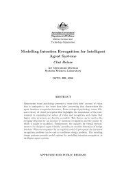
DSTO–TN–0640nθx ′xFigure 4: The matrix R n (θ) rotates x in a right-handed sense around theunit vector n by an angle θ to produce x ′ . That is, x ′ = R n (θ) xwhere n can point in either direction along the axis, but changing the choice of that directionwill change the sign required for the rotation angle θ, since the rotation matrix R n (θ)obeys the right hand rule for rotation. The rotation matrix can be written in the followingway, which is the main equation of this report:⎡⎤⎡⎤n 2 1 n 1 n 2 n 1 n 3R n (θ) = (1 − cos θ) ⎣n 2 n 1 n 2 2 n 2 n 3⎦ + cos θ I 3 + sinθ ⎣n 3 n 1 n 3 n 2 n 2 30 −n 3 n 2n 3 0 −n 1⎦−n 2 n 1 0= (1 − cos θ) nn t + cos θ I 3 + sin θ n × , (3.7)where n t is the transpose of n, I 3 is the 3 × 3 identity matrix, and⎡⎤0 −n 3 n 2n × ≡ ⎣ n 3 0 −n 1⎦ , (3.8)−n 2 n 1 0so-named becausen × x = n × x, (3.9)(with the n written nonbold to emphasise its matrix form). The rotation matrix R n (θ)is called orthogonal, by which is meant RR t = R t R = 1, and as well its determinant isalways 1. Equation (3.7) will be used repeatedly in this report to break more complicatedprocedures up into single rotations that are easy to visualise and easy to code. It is, infact, the central equation of the whole of rotation theory.Example of the use of (3.7): Rotate the vector (2, 0, 0) by 90 ◦ about the y-axis.What vector results? The required rotation matrix is R y (90 ◦ ) (where by the subscript yis meant n = (0, 1, 0) t ). Equation (3.7) gives it as⎡ ⎤ ⎡ ⎤ ⎡ ⎤0R y (90 ◦ ) = nn t + n × = ⎣1⎦ [ 0 1 0 ] + ⎣00 0 10 0 0⎦ = ⎣−1 0 00 0 10 1 0⎦ . (3.10)−1 0 0(Actually, in this simple example we can calculate R y (90 ◦ ) alternatively using (3.2). Simplynote that the basis vectors rotate as⎡ ⎤ ⎡ ⎤ ⎡ ⎤ ⎡ ⎤ ⎡ ⎤ ⎡ ⎤1 0 0 0 0 1⎣0⎦ −→ ⎣ 0⎦ , ⎣1⎦ −→ ⎣1⎦ , ⎣0⎦ −→ ⎣0⎦ , (3.11)0 −1 0 0 1 08