An Introduction to Free-space Optical ... - Radioengineering

RADIOENGINEERING, VOL. 19, NO. 2, JUNE 2010 203
An Introduction to Free-space Optical Communications
Hennes HENNIGER 1 , Otakar WILFERT 2
1 Institute of Communications and Navigation, German Aerospace Center (DLR), 82230 Wessling, Germany
2 University of Technology Purkynova 118, CZ-61200 Brno, Czech Republic
Abstract. Over the last two decades free-space optical
communication (FSO) has become more and more interesting
as an adjunct or alternative to radio frequency communication.
This article gives an overview of the challenges
a system designer has to consider while implementing an
FSO system. Typical gains and losses along the path from
the transmitter through the medium to the receiver are introduced
in this article. Detailed discussions of these topics
can be found in this special issue of the Radioengineering
Journal.
Keywords
Free-space optical communications, link budget, turbulence,
fading.
1. Introduction
Free-space optical communication (FSO) systems (in
space and inside the atmosphere) have developed in response
to a growing need for high-speed and tap-proof communication
systems. Links involving satellites, deep-space probes,
ground stations, unmanned aerial vehicles (UAVs), high altitude
platforms (HAPs), aircraft, and other nomadic communication
partners are of practical interest. Moreover, all
links can be used in both military and civilian contexts. FSO
is the next frontier for net-centric connectivity, as bandwidth,
spectrum and security issues favor its adoption as an adjunct
to radio frequency (RF) communications [1].
While fixed FSO links between buildings have long
been established and today form a separate commercial
product segment in local and metropolitan area networks
[2], the mobile and long-range applications of this technology
are aggravated by extreme requirements for pointing and
tracking accuracy because of the small optical beam divergences
involved. This challenge has to be addressed to fully
exploit the benefits of optical links. Furthermore, long-haul
optical links through the atmosphere suffer from strong fading
as a result of index-of-refraction turbulence (IRT) and
link blockage by obscuration such as clouds, snow and rain.
In this article an overview of the challenges a system
designer has to respond to when implementing an FSO sys-
henniger@ieee.org, wilfert@feec.vutbr.cz
tem is provided. Typical gains and losses along the path from
the transmitter through the medium, to the receiver are introduced
in this article. Some results concerning the qualitative
parameters of the links and statistical characteristics of the
atmosphere are described.
A more detailed discussion and further information on
these topics can be found in papers in this special issue of
the Radioengineering Journal.
2. Discussion of Selected Modulation
Schemes
The optical carrier can be modulated in its frequency,
amplitude, phase, and polarization. The most commonly
used schemes because of their relatively simple implementation
are amplitude modulation with direct detection and
phase modulation in combination with a (self-)homodyne or
heterodyne receiver.
The technically simplest digital modulation scheme is
amplitude-shift keying (2 ASK). In optical systems it is referred
to as on-off keying (OOK). OOK is an intensity modulation
scheme where the light source (carrier) is turned on
to transmit a logic ”one” and turned off to transmit a ”zero”.
In its simplest form this modulation scheme is called NRZ
(non-return-to-zero)-OOK. Besides NRZ also other codes
exist. The most common one besides NRZ is RZ (returnto-zero)
coding. The advantages of RZ compared to NRZ
are its higher sensitivity [3] and the fact that the clock frequency
lies within the modulation spectrum. Unfortunately,
both NRZ and RZ can lead to loss of clock synchronization
if long strings of ones or zeros are transmitted. This can be
avoided with other coding systems such as Manchester coding,
which is related to RZ but amounts to state changes at
the beginning or in the middle of clock cycles - pulse position
modulation. With such a variant of RZ the clock of
the digital signal can easily be recovered. These advantages
come at the cost of a requirement of twice the bandwidth of
NRZ in order to fulfill the Nyquist–Shannon theorem. Nevertheless,
it has been shown, for example in [4], [3], that RZ
can also work when using the same bandwidth as for NRZ.
In this case an increase in sensitivity of about 2 dB has been
reported [4].
Furthermore, line codes are often used to guarantee that

204 H. HENNIGER, O. WILFERT, AN INTRODUCTION TO FREE-SPACE OPTICAL COMMUNICATIONS
the short time average of the signal (i.e., the ”baseline”) is
constant. This is important because optical amplifiers need
input signals with constant mean power if they work with
control loops to guarantee constant mean output power. Further
AC-coupling (high-pass filtering) of the electrical signal
at the receiver will introduce a significant amount of
inter-symbol interference if the average of the signal is not
constant [5]. Therefore 8B10B coding on top of NRZ is
commonly used in fiber systems and can also be applied to
FSO systems. For 8B10B-NRZ the bandwidth requirement
is only 25 percent more than for NRZ. An additional advantage
8B10B coding has is that this coding forces frequent
level changes independent of the input stream. Therefore
the clock of the signal can easily be recovered even if long
strings of ”ones” or ”zeros” are transmitted.
For OOK, the exact wavelength of the carrier and its
phase are irrelevant for the demodulation. The receiver just
directly detects the currently incoming power and compares
it against a certain level. OOK is sensitive to amplitude
distortion (fading) and propagation through different routes,
while the second one is negligible for clear-sky conditions.
Atmospheric obscuration e.g. in clouds can lead to significant
attenuation of the received signal but is less important
for FSO systems operating under clear-sky conditions.
Coherent modulation systems are also used in optical
communications. Usually, a binary coherent modulation
scheme is used. For example binary phase shift keying
(BPSK), where the phase of the coherent laser light is shifted
between two states. Coherent receivers rely on the superposition
of the received light with the light of a local oscillator.
Instead of the local oscillator self-homodyne is alo possible.
This is used in differential phase shift keyed (DPSK) systems,
which are less sensitive than BPSK systems. In BPSK
systems typically some kind of optical phase-locked loop is
required, which allows the local oscillator laser to be tuned
exactly to the same frequency (or a frequency with a constant
offset) and phase as the received carrier. The sensitivity of
coherent receiver implementations is approximately one to
two orders of magnitude better than the sensitivity of OOK
systems [6], [7] but at the cost of higher system complexity
and additional sensitivity to phase distortions of the received
beam.
Generally, an OOK system is more robust with regard
to atmospheric distortion than a coherent modulation system.
This is because for OOK the information is only encoded in
intensity whereas PSK uses intensity and phase coding. Both
the intensity and the phase of a beam are disturbed in atmospheric
propagation. Further, OOK has mainly been used in
optical fiber communications due to its low complexity. Additionally,
many reliable and cost effective components are
available in the market, which is important for the development
of FSO communication terminals. As a result, OOK
systems have been preferred for optical links inside the atmosphere:
they are the primary focus of this article.
Since the electrical signal in OOK receivers is propor-
tional to the received optical power, all further calculations
can be carried out based on the statistics of the received optical
power focused on the receiver photodetector.
3. The Optical Link Equation
The overall system performance of a link is quantified
using a link margin derived from the link equation. The optical
link equation is analogous to the link equation for any
radio frequency (RF) communication link. Starting with the
transmit power the designer identifies all link degradations
and gains to determine the received signal level. The received
signal level is then compared with the sensitivity of
the receiver, thus giving the link margin.
3.1 Channel Without Atmospheric
Disturbance
In this section optical links unaffected by the atmosphere
are discussed. In the basic free-space channel the optical
field generated at the transmitter propagates only with
an associated beam spreading loss. For this system the performance
can be determined directly from the power flow.
The signal power received PRx [W] depends on the transmit
power PT x [W], transmit antenna gain GT x, receive antenna
gain GRx, the range loss Gr, and system-dependent losses
Asystem,lin.
PRx = PT x · GT x · Gr · GRx · Asystem,lin. (1)
Assuming a Gaussian beam underfilling the transmit
aperture, the transmit antenna gain GT x is ([8], page 99):
GT x = 32
Θ 2
where Θ [rad] is the full-angle e −2 divergence of the transmit
beam.
The range loss Gr depends on the link propagation distance
L and is given by:
� �2 λ
Gr = . (3)
4π · L
Further, the receive antenna gain, with telescope aperture
diameter (antenna size) D, is given by [6]:
� �2 π · D
GRx = . (4)
λ
The Asystem,lin reflects all the other system-dependent
losses. It includes losses due to link misalignment, telescope
losses, losses due to splitting out light for tracking systems,
etc.
Because of the absence of atmospheric effects the link
margin Mlink in dB is given by:
Mlink[dB] = PRx,dBm − Sr
(2)
(5)

RADIOENGINEERING, VOL. 19, NO. 2, JUNE 2010 205
where received power PRx,dBm [dBm] must be given on a logarithmic
scale. Sr [dBm] is the required power at the receiver
to achieve an expected communication performance,
also called receiver sensitivity. It depends on several constraints,
for example data rate and the required bit error probability.
Sensitivity depends on noise sources influencing the
detection, such as ambient light and electronic noise. Similar
power budget analyses of the link are described in prior publications
[9], [10], [11], [12]. The power balance equation
can be expressed with the help of the power level diagram
[9].
To consider the effects disturbing a link propagating
through the Earth’s atmosphere the link equation (5) must
be extended. The primary atmospheric processes that affect
optical wave propagation are extinction and refractive index
turbulence (IRT). The main problems of optical communication
in the atmosphere are attenuation of optical intensity
and fluctuations of received optical signal. An attenuation of
optical intensity is caused by the absorption, scattering and
refraction of optical waves by gas molecules and aerosols
such as fog, snow and rain. Especially for short links heavy
fog is the main factor that limits the link function. For link
lengths exceeding several hundred meters fluctuations of received
optical signal present a severe problem.
Signal fluctuations of the received signal PRx can in
some time intervals fall below the receiver sensitivity Sr. In
such time intervals a so-called “fade” of the signal occurs.
The effects of atmospheric extinction, atmospheric turbulence
and fades are introduced in the following two sections.
3.2 Atmospheric Extinction Effects
It is well known that clouds, rain, snow, fog, haze, pollution
etc. are atmospheric factors that affect our viewing of
distant objects. These same factors also affect the transmission
of a laser beam through the atmosphere. As transmission
through clouds or heavy fog or haze is normally not possible,
because attenuation exceeds several tens of dB/km,
this is not discussed in this paper. Nevertheless, the signal
under clear-sky weather conditions is attenuated because of
extinction caused by air molecules and aerosols. The transmittance
T of laser radiation that has propagated over a distance
L is described by the Beer’s law:
T = exp(−αe(λ) · L[km]). (6)
The positive extinction coefficient αe(λ) describes the
extinction level of the medium. It is usually given in km −1
and is commonly available in databases like LOWTRAN
[13] or others like FASCODE , MODTRAN, HITRAN, for
example described in [14]. It turns out that the extinction
is highly wavelength-dependent. Atmospheric trace gases
lead to strong and broad absorption bands, each consisting
of a multitude of fine absorption lines. Based on the spectral
distribution of these bands, the so called atmospheric
optical transmission windows with low signal losses of the
propagating beam can be calculated by evaluating thousands
of absorption lines in the spectral range from 0.3 µm to
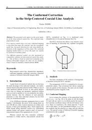
14 µm. A description of the atmospheric transmission windows
based on extensive evaluation of various data-bases
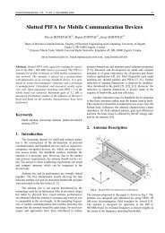
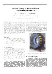
[15], [16], [17], is given in Tab. 1 and Fig. 1. It can be
seen that typical terrestrial communication wavelengths like
808 nm (Si detectors), 1064 nm (Nd-YAG lasers) or 1550 nm
(InGaAs detectors, erbium-doped fiber amplifiers) are applicable,
whereas 950 nm and 1300 nm are not ideal for FSO
systems.
I II III IV V VI VII VIII
0.30 0.97 1.16 1.40 1.95 3.00 4.5 7.7
0.92 1.10 1.30 1.80 2.40 4.20 5.2 14
Tab. 1. Atmospheric Optical Transmission Windows (Window
start- and stop-wavelength given in µm).
In addition to absorption, scattering has also to be taken
into account. This can be described by the Rayleigh scattering
coefficient [18]. Generally, scattering effects decrease
monotonically with wavelength and altitude.
Even in optical windows some extinction must be considered,
e.g. due to Rayleigh scattering. A rough estimate
for the clear-sky extinction is based on the meteorologic parameter
visibility V . This can be given by the Kruse relation
[19], [20]. The Kruse relation, which is modified to reflect
the attenuation in decibel per kilometer, is given by:
Ae[dB/km] = 17
V [km] ·
� �q 0.55
≥ 0
λ[µm]
where the exponent q is given by
⎧
⎪⎨ 1.6, if V > 50 km,
(7)
q = 1.3,
⎪⎩
0.585 ·V
if 6 km ≤ V ≤ 50 km,
1 3 , if V < 6 km.
(8)
As well as the Kruse relation there are also other models,
as for example presented by the papers in this issue of the
Radioengineering Journal. Further, [21] proposed another
expression for the parameter q, which was given by Kruse as
defined in equation (8). Naboulsi et. al. in their work [22]
developed relations using the atmospheric database FAS-
CODE to evaluate the attenuation in the 690 nm to 1550 nm
wavelength range.
Coming back to the link equation, (5) must be modified
by Ae [dB/km] in order to consider extinction effects of the
atmosphere:
Mlink[dB] = PRx,dBm − Sr − L[km] · Ae. (9)
In the near-earth layer, rainfall and snow can also reduce
the link margin and must be considered in the link equation
(9). Several models exist to estimate the attenuation due
to rainfall and snow. These models can be found for example
in the standardization documents of the International
Telecommunication Union [20].
In addition to extinction effects, fading effects produced
by the atmosphere must also be considered. This is
discussed in the following.

206 H. HENNIGER, O. WILFERT, AN INTRODUCTION TO FREE-SPACE OPTICAL COMMUNICATIONS
Fig. 1. Atmospheric transmittance based on absorption analysis using LOWTRAN [13]. A zenith path from 0 km to 120 km altitude as well as
the midlatitude summer atmospheric model are assumed. Atmospheric transmission windows are highlighted in grey color.
3.3 Influence of Turbulence
This section is divided into two parts. First physical
beam propagation is discussed. Second the reception process
of a distorted wave is discussed and the impact on the
communication system is given.
Physical Effects of Optical Beam Propagation Through
Random Media: Random variations of the refractive index -
also known as index-of-refraction turbulence (IRT) - of the
Earth’s atmosphere are responsible for wavefront distortion.
Thus, if a beam with a longitudinal coherence length of at
least several wavelengths propagates through IRT the intensity
of the original beam profile is redistributed. For example,
a Gaussian-shaped intensity profile is transformed into a
random interference pattern, the so-called intensity speckle
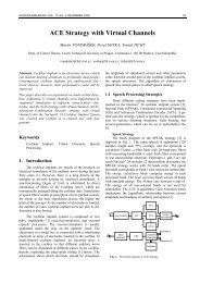
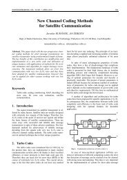
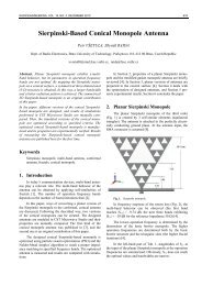
pattern. Cross-sections of the beam before and after propagation
through the atmosphere are shown in Fig. 2. As the
refractive index structure along the path is time dependent
because of the turbulent mixing of refractive index cells, the
spatial intensity distribution at the receiver plane varies. The
temporal variation of intensity observed at an infinitely small
point and the spatial variation of intensity within the receiver
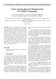
aperture are commonly described as ”scintillation”. The in-
tensity scintillation-index σ 2 I
is the normalized variance of
the intensity and is used as a measure of scintillations. The
scintillation-index is usually evaluated in terms of the β 2 0 -
parameter, which is an analytical measure for the integrated
amount of turbulence along the link path. It shall be noted
-parameter equals
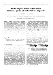
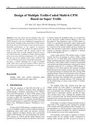
that for weak fluctuations (σ2 I < 0.3) the β20 the Rytov variance. Fig. 3 shows the intensity scintillationindex
σ2 I as a function of β2 0 of a spherical wave1 under general
irradiance fluctuation conditions2 . In strong turbulence
or along long paths the scintillation-index saturates. Saturation
occurs because multiple scattering can cause the incident
wave to become increasingly incoherent as it propagates
through the medium. A single source of light can, therefore,
appear as extended multiple sources scintillating with
random phase. When these multiple apparent source fields
are added, the resultant intensity scintillation is limited [24].
Thus, for a low level of turbulence single scattering, which
deflects light from the main beam, causes weak scintillation.
For an increasing amount of turbulence more multiple scattering
occurs. Multiple scattering can deflect light from the
main beam but as turbulence gets stronger is can actually deflect
the light back into the main beam again. Therefore the
scintillation saturates.
For a horizontal path (spherical wave) β2 0 is given
by [25]:
β 2 0 = 0.496 ·C 2 n · k 7/6 · L 11/6 . (10)
1 In the case of mobile links or static links without active pointing and tracking inside the atmosphere we usually deal with spherical waves, because the
transmit-beam divergence has to expand above the diffraction-limited value to ensure illumination of the partner terminal from an unstable moving platform.
Spherical waves are therefore used as the examples here, but the theory presented is not limited to these kinds of waves. The classification of the transmitted
beam as a spherical wave holds when the full e −2 divergence angle Θ in radians is larger than 7.1 · � λ/L, as can be deduced from the theory given in [23],
page 180, by using an arbitrarily chosen classification limit.
2 The non general case is the case when the Rytov approximation holds. This approximation is only true for weak fluctuations. The Rytov approximation
assumes that wave distortions caused by the turbulence encountered early on in the propagation path will not have any influence on the distortions caused by
turbulence countered further on the propagation path.

RADIOENGINEERING, VOL. 19, NO. 2, JUNE 2010 207
Fig. 2. Laser beam propagation through turbulent atmosphere:
intensity cross-section of the transmit beam (left), intensity
cross-section at the receiver plane (right).
Here, k = 2π is the optical wave number, L [m] is again the
λ
propagation path length and C2 n is the refractive index structure
parameter. C2 n is the structure constant of refractive index
fluctuations and a measure of the turbulence strength,
given in m−2/3 . It depends strongly on the height above
ground ha. Nevertheless, for applications involving propagation
along a horizontal or quasi-horizontal path, C2 n can
be assumed to be constant, especially for near-ground links
were the variance in altitude due to the Earth’s curvature
is negligible. At near ground level, C2 n values will show
a diurnal cycle, which peaks during midday hours, reaches
near-constant values at night, and has minima near sunrise
and sunset. This behavior is documented by measurements,
which can be found for example in [6], [24], [26].
Fig. 3. Intensity scintillation-index σ 2 I as a function of β2 0 under
genearal irradiance fluctuaion conditions. According to
equation found in [25], page 39.
The Hufnagel-Vally model [23] provides a model often
used by researchers to describe the altitude dependence of
C 2 n(ha) in rural areas. The H-V 5/7 variant of the Hufnagel-
Vally model is given by
C 2 n(ha) =
0.00594 � 21
27
� �
2 ha ·
105 �10 m
m−2/3 �
· exp
+2.7 · 10−16 m−2/3 �
· exp − ha
�
1500 m
+1.7 · 10−14 m−2/3 �
· exp − ha
�
100 m .
− ha
1000 m
�
(11)
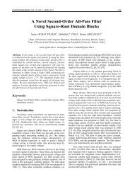
Height dependent values of C 2 n based on the H-V 5/7
model are given in Fig. 4. The Hufnagel-Valley model gives
an averaged C 2 n-value for a certain altitude. In reality, C 2 n
shows various small scale variations with altitude. C 2 n profiles
have been studied extensively, and beside the Hufnagel-
Vally model various other theoretical models have been proposed
in the past. They can be found for example in [24],
[23].
IRT above water differs from that above soil due to the
fact that energy exchange on the ground is controlled almost
exclusively by molecular conduction. In water, however,
there is an additional exchange of mass and heat transfer at
the air-water interface by convection (vertical sensible heat
flux), advection (horizontal heat flux) and evaporation (lateral
heat flux) [27]. The potential rate of evaporation is determined
by the air-sea temperature difference (ASTD) and
the state of the air. Slight roughness of the water surface
modifies the wind field above water and ocean waves enhance
vertical mixing.
Because of the large thermal capacity of water, it requires
much more energy to raise the temperature of a volume
of water than for most soils. Therefore ASTD is smaller
than the temperature difference between most other natural
surfaces. Furthermore, the daily fluctuations of the water
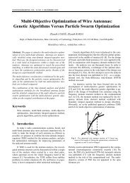
surface temperature will be small. In general, the C 2 n values
above water are smaller than expected above land (compare
Fig. 4) and diurnal variations are less pronounced,
e.g. maximum C 2 n can not everytime be expected at midday.
Majumdar provides in his work [6] a maritime turbulence
profile model for altitudes up to 6000 m. Parameter
sets for three cases are provided: best C 2 n(h = 0 m)
= 1 · 10 −16 m −2/3 , median C 2 n(h = 0 m) = 8 · 10 −16 m −2/3 ,
and worst C 2 n(h = 0 m) = 1 · 10 −14 m −2/3 . These cases reflect
the dependence of C 2 n on the condition of the air-sea interface.
The model is in good agreement with the measured
values given in [27]. The medium profile maritime − C 2 n
model, which is valid for ha < 6000 m is given by [6] as
C2 n(ha) =
9.8583 · 10−18 m−2/3 +4.9877 · 10−16 m−2/3 �
· exp − ha
�
300 m
+2.9228 · 10−16 m−2/3 �
· exp − ha
�
1200 m .
(12)
This maritime −C 2 n profile is shown in Fig. 4 in comparison
with the rural H-V 5/7-model. It can be seen that
above 500 m there is not much difference between the two
models, because the influence of the boundary layer is negligible.
A strong and temporarily changing gradient in the
index-of-refraction on the link can cause a deflection of an
optical wave from a straight-line trajectory. Such a refraction
causes very slow but relatively strong fluctuations in the angle
of arrival of the beam at the receiving aperture. To eliminate
this effect an active beam steering and tracking system
is necessary, even for stationary links.
Reception of Distorted Wavefront: As given in the preceding
section, atmospheric propagation disturbs the beam
profile, which means that the wavefront of the optical beam
is distorted. Receiving this distorted wavefront will cause
signal fading. The fading effect and the necessary margin to

208 H. HENNIGER, O. WILFERT, AN INTRODUCTION TO FREE-SPACE OPTICAL COMMUNICATIONS
Fig. 4. Rural C 2 n as a function of hight above ground h according
to the Hufnagel-Valley H-V 5/7-model in comparison
with a maritime −C 2 n model.
overcome it are discussed in this section.
In optical receiver systems the energy in the beam is
collected by a receive aperture. We consider circular receiver
apertures defined by the function:
fRx(r,D) =
�
1, if |r| ≤ D 2 ,
0, if |r| > D 2
(13)
where D is the diameter of the receiver aperture. It is typically
in the range of several centimeters to tens of centimeters.
r is the radial distance from the optical axis. We assume
long-range communication links, where the optical signal
spot at the receiver plane is several times larger than the aperture
diameter D. In this case the received signal amplitude
equals the integral of optical intensity I(r,t) over area.
�� ∞
PRx(t) = fRx(r,D) · I(r,t)d
−∞
2 r. (14)
The effect of integrating over the intensity reduces the
deleterious effects of scintillation. This reduction is called
aperture averaging. Qualitatively, we can regard the aperture
as consisting of an array of nonoverlapping regions. Within
each region the scintillations are perfectly correlated while
between the regions there is no significant correlation. The
regions are also called speckle. For horizontal paths a rough
estimate for the speckle size at the receiver is given by the
communication wavelength and the link distance: √ L · λ [6].
If the aperture is larger than the speckle size, then uncorrelated
scintillations from many regions will be averaged together,
thereby reducing the signal dynamics.
The variance of received power σ2 P scaled by the square
of the mean power 〈PRx〉 is called the power scintillationindex.
The ratio of the irradiance flux variance obtained by
a finite-size receiver lens to that obtained by a point receiver
is called the aperture-averaging factor fAA:
fAA = σ2P σ2 , 0 < fAA < 1. (15)
I
The aperture-averaging factor quantifies the reduction
of scintillation.
Amplitude fading, even if aperture-averaging is taken
into consideration, can be described by statistical models
showing the probability density function (PDF) of the received
signal. Analysis presented in [28]-[33] shows that
the log-normal (LN) statistical model generally adequately
describes the amplitude-fading of the received signal. Beside
the LN model several other models have been reported
in the literature, e.g. gamma-gamma [31], [34], [35] or
K-distribution [29], [36], [37], and may provide a better
description in very strong turbulence, but their distribution
functions are mathematically more complicated. Nevertheless,
measurements with real existing systems presented in
[32], [33] confirm, that the LN statistical model adequately
describes the dynamics of the received power signal. Therefore,
in the following LN-fading statistics are discussed.
Generally, the PDF of the received analog signal H is modeled
by the LN distribution:
1
fH LN(h) = �
h · 2πσ2 �
[lnh − µLD]
2
exp −
2σ
LD
2 �
,h > 0 (16)
LD
The parameters of the LN distribution µLD and σ 2 LD are
the mean value and the variance of the underlying normal
distribution, respectively. The expectation value of the LN-
PDF E[H] is also the expectation value of the received signal
E[H].
E[H] = exp(µLD + σ2 LD )
2
(17)
The well known (general) scintillation-index σ2 SI 3 is defined
by
σ 2 SI = Var[H]
.
(E[H]) 2 (18)
It directly depends on LN distribution parameter σ 2 LD
σ 2 SI = exp(2µLD + σ2 LD )(exp(σ2LD ) − 1)
(exp(µLD + 1 2σ2 LD ))2
= exp(σ 2 LD) − 1
(19)
and specifies the LN-PDF fH LN(h). If fH LN(h) models the
distribution of the received power the (general) scintillationindex
σ2 SI must be substituted by the power scintillationindex
σ2 P .
Further, it is operationally satisfactory to substitute in
(16) h = PRx where PRx > 0 and therefore (16) becomes 4
fPRx LN(PRx) =
PRx ·
1
�
2πσ2 �
exp −
LD
PRx [ln 〈PRx〉 − µLD]
2
2σ2 LD
3 The (general) scintillation-index σ2 SI can be replaced by the power scintillation-index σ2 P if the signal H describes the received power PRx or by the
intensity scintillation-index σ2 I if the intensity PDF is given. The power equals the integrated intensity over the receiver aperture; compare (14) .
4 As the area below the probability density function must be equal to unity the equation must be normalized by the mean power after the substitution.
�
(20)

RADIOENGINEERING, VOL. 19, NO. 2, JUNE 2010 209
In what follows, all received power values are assumed
to be normalized to the mean value 〈PRx〉. In this case the
parameters of the LN-distribution for the received power are
given by:
σ 2 LD = ln � σ 2 P + 1 � , (21)
µLD = − σ2LD . (22)
2
In general, based on a knowledge of the received power
distribution fPRx a system outage probability pB can be calculated.
If the communication system is assumed to work
properly when the receiving power is greater than the receiver
sensitivity Sr the probability of system outage (fractional
fade time) is a cumulative density function (CDF).
pB(Sr) =
� Sr
fPRx
0
(PRx) dPRx. (23)
The required power margin between the average reception
power 〈PRx〉 and Sr (Sr < 〈PRx〉) must be regarded as an
additional fading loss A f ade of the transmission system.
A f ade[dB] = 10 · lg 〈PRx〉
Sr
≥ 0 (24)
With this threshold approach it is assumed that during
times with PRx below Sr no data reception is possible at all.
This reflects a good-bad-state channel modeling and does
not require a detailed investigation of the specific receiver
performance; the latter would again depend on the modulation
format and individual implementation performance. In
connection with the good-bad-state channel model the fractional
fade time pB can also be called outage probability or
bad-state probability.
If PRx is LN distributed one obtains the fractional fade
time pB based on equation (20) and in analogy to [30], [28],
[23].
pB(Sr) = frac [P ≤ Sr] (25)
= 1
� � ��
Sr ln 〈PRx〉 − µLD
1 + erf
(26)
2
√ 2σLD
where erf(.) denotes the error function. To calculate the fading
loss the equation (26) must be solved for
Sr
〈PRx〉 :
�√ Sr
= exp 2σLD · erf
〈PRx〉 −1 (2pB − 1) + µLD
�
. (27)
The fading loss A f ade on a logarithmic scale is therefore
given by
A f ade[dB] �= √2σLD −10lge · · erf−1 �
(2pB − 1) + µLD .
(28)
With the assumption E[PRx] = 1 and the approximation
10lge � 4.343, (28) reduces to:
A f ade(σ2 P , pB)[dB] ��
=
−4.343 2ln(σ2 P + 1) · erf−1 (2pB − 1) − 1 2 ln(σ2 �
P + 1)
(29)
Therefore, the fading loss is determined by the power
scintillation-index σ2 P and allowed fractional fade time
pB(Sr).
(29) describes the loss or margin which must be considered
in link design in order to obtain a certain fractional
fade time. Therefore, the link equation from (5), (9), respectively,
must be extended by A f ade in order to consider IRT
fading:
Mlink[dB] = PRx,dBm − Sr − L[km] · Ae − A f ade. (30)
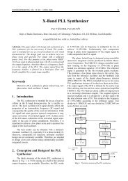
Fig. 5. Fading loss A f ade vs. power scintillation-index σ 2 P as
a function of fractional fade time pB.
As can be observed in Fig. 5 the fading loss according
to (29) can easily exceed 20 dB with typical link requirements
(e.g. with outage probabilities of 10 −6 ). Further, for
moderate outage requirements (> 10 −3 ) with turbulence saturation
and aperture averaging the loss will rarely exceed
13 dB. Saturation means that for long distances the intensity
scintillation index σ2 I is saturated near or somewhat above
unity while the power scintillation-index σ2 P becomes less
than unity because of aperture averaging [33], [28].
Finally, having introduced all the main factors disturbing
a free-space optical link inside the atmosphere we can
calculate link budget based on (30). An exemplary link budget
for a 20 km horizontal link is shown in Fig. 6.
Fig. 6. Exemplary link budget base on link equation (30) [38].
Further we evaluate the influence of IRT induced
fading-loss versus link range. Therefore we chose the fol-

210 H. HENNIGER, O. WILFERT, AN INTRODUCTION TO FREE-SPACE OPTICAL COMMUNICATIONS
lowing link parameter: C 2 n(ha = const.) = 1 · 10 −14 m −2/3 ,
λ = 1550 nm, Θ = 1 mrad, D = 5 cm, pB = 10 −2 ,
PT x = 500 mW, Asystem,lin = 0.5, Ae = 0.2 dB/km, and
a typical receiver sensitivity for a 155 Mbit/s system of
Sr = −43 dBm. Fig. 6 shows the link margins according
to (9) and (30). As described earlier, with increasing link
length the integrated amount of turbulence increases. This
first causes the scintillation-index to increase steadily, then
a maximum is observed and finally it saturates. As shown
in the lower plot in Fig. 6, the fading-loss according to (29)
behaves in a way analogous to the scintillation-index. It first
increases, peaks, and is than nearly constant for longer distances.
Fig. 7. Upper plot: Link margin including the effect of fading
cause by IRT in comparison to a case without atmospheric
fading. Lower plot: Scintillation-index and
fading-loss versus link distance in comparison to the link
margin of the upper plot.
If the basic parameters of the given link are known, it is
possible to use (5) and obtain link margin Mlink as a function
of link propagation distance L. Such a relationship represents
the steady state model of the given link. In addition, if
the statistical character of the atmosphere at the chosen installation
site of the link is known, it is possible to obtain
the probability of atmospheric attenuation exceeding a given
value that represents the statistical model of the chosen link
installation site. With the help of synthesis of the steady state
model of a given link and the statistical model of the chosen
installation site we can obtain the so-called complex model
of the link. Statistical characteristics of the atmosphere in
some localities in Europe were published in [11].
3.4 Conclusion
A brief survey of the fundamentals of FSO has been
presented in this introductory article. This brief survey has
focused on outdoor FSO static optical links and describes
some basic models of the link and some simple models of
the atmosphere.
The advantages of FSO result from the basic characteristics
of a laser beam, especially from its high frequency,
coherency and low divergence, which lead to efficient deliv-
ery of power to a receiver and a high information-carrying
capacity.
The basic characteristics of a laser beam provide the
following additional advantages of FSO links:
• A narrow beam guarantees high spatial selectivity so
there is no interference with other links.
• The high available bit rate allows them to be applied in
all types of networks.
• The optical band lies outside the area of telecommunication
regulation; therefore no license is needed for
operation.
• The small size and small weight of optical terminals enables
links to be easily integrated into mobile systems.
Nevertheless, challenges remain. The main problems
of FSO links working outdoors in the atmosphere result from
attenuation and fluctuation of optical signal at a receiver. To
improve reliability, a number of new methods are being applied.
For example, a hybrid FSO/RF system increases link
availability by overcomming attenuation effects. RF transmission
is affected more by rain and optical transmission is
affected more by fog. Further, error protection schemes able
to deal with the slow fading typical for FSO links are currently
under development.
After considering all its advantages and disadvantages
it is clear that FSO has good prospects for widespread implementation.
FSO technology is ready for utilization as terrestrial
links, mobile links and satellite links.
Acknowledgements
The authors would like to thank Professor Christopher
C. Davis (University of Maryland) for his help and fruitful
discussions.
The research leading to these results has received funding
from the European Community’s Seventh Framework
Programme (FP7/2007-2013) under grant agreement no.
230126 and from the Research programs of the Czech Science
Foundation No. 102/09/0550.
References
[1] DAS, S., HENNIGER, H., EPPLE, B., MOORE, C., RABINOVICH,
W., SOVA, R., YOUNG, D. Requirements and challenges for tactical
free-space lasercomm. In IEEE Military Communications Conference
. San Diego (USA), 2008, p. 1 – 10.
[2] WILLEBRAND, H., GHUMAN, B. Fiber optics without fiber. IEEE
Spectrum, 2001, vol. 38, no. 8, p. 40 – 45.
[3] PAUER, M., WINTER, P., LEEB, W. Bit error probability reduction
in direct detection optical receivers using rz coding. Journal of Lightwave
Technology, 2001, vol. 19, no. 9, p. 1255 – 1262.

RADIOENGINEERING, VOL. 19, NO. 2, JUNE 2010 211
[4] LEEB, W., WINTER, P., PAUER, M. The potential of return-to-zero
coding in optically amplified lasercom systems. In IEEE Lasers and
Electro-Optics Society 1999 12th Annual Meeting LEOS ’99, vol. 1.
San Francisco (USA), 1999, p. 224 – 225.
[5] STREET, A., SAMARAS, K., OBRIEN, D., EDWARDS, D. Closed
form expressions for baseline wander effects in wireless ir applications.
Electronics Letters, 1997, vol. 33, no. 12, p. 1060 – 1062.
[6] MAJUMDAR, A. K., RICKLIN, J. C. Free-Space Laser Communications
Principles and Advances. Sew York (USA): Springer, 2008.
[7] DAVID, F. Scintillation loss in free-space optic im/dd systems. In
LASE 2004, vol. 5338. San Jose (USA), 2004.
[8] LAMBERT, S. G., CASEY, W. L. Laser Communications in Space.
Boston (USA): Artech House, 1995.
[9] WILFERT , O., KOLKA, Z. Statistical model of free-space optical
data link. Proceedings of SPIE, 2004, vol. 5550, p. 203 – 213. [Online]
Available at: http://link.aip.org/link/?PSI/5550/203/1
[10] WILFERT, O., KOLKA, Z., NEMECEK, J., BIOLKOVA, V. Estimation
of fso link availability in Central European localities. Proceedings
of SPIE, 2006, vol. 6303, p. 63030R. [Online] Available at:
http://link.aip.org/link/?PSI/6303/63030R/1
[11] KOLKA, Z., WILFERT, O., FISER, O. Achievable qualitative parameters
of optical wireless links. Journal of Optoelectronics and
Advanced Materials, 2007, vol. 9, no. 8, p. 2419 – 2423.
[12] KOLKA, Z., WILFERT, O., KVICALA, R., FISER, O.
Complex model of terrestrial fso links. Proceedings of
SPIE, 2007, vol. 6709, p. 67091J. [Online] Available at:
http://link.aip.org/link/?PSI/6709/67091J/1
[13] KNEIZYS, F. X. Atmospheric Transmittance/Radiance [Microform]:
Computer Code LOWTRAN 6. Bedford (USA): Hanscom
AFB, 1983.
[14] SMITH, F. G., ACCETTA, J. S., SHUMAKER, D. L. The Infrared
& Electro-Optical Systems Handbook. Atmospheric Propagation
of Radiation, Vol. 2. SPIE Press, 1993. [Online] Available at:
http://www.scribd.com/doc/13650098/IR-Handbook-Volume-2
[15] EDWARDS, D. P. GENLN2: A General Line-by-Line Atmospheric
Transmittance and Radiance Model. Version 3.0: Description and
users guide (technical report). National Center for Atmospheric Research,
1992.
[16] MAYER, B., SHABDANOV, S., GIGGENBACH, D. Atmospheric
Database of Atmospheric Absorption Coefficients (technical report).
German Aerospace Center (DLR), 2002.
[17] MAYER, B., KYLLING, A. Technical note: The libradtran software
package for radiative transfer calculations - description and examples
of use.’ Atmospheric Chemistry and Physics, 2005, vol. 5,
no. 7, p. 1855 – 1877. [Online] Available at: http://www.atmoschem-phys.net/5/1855/2005/
[18] HENNIGER, H., GIGGENBACH, D., RAPP, C. Evaluation of optical
up- and downlinks from high-altitude platforms using im/dd. In
LASE 2005, Free-Space Laser Communications Technologies XVII.
San Jose (USA), 2005.
[19] KRUSE, P. W., MCGLAUCHLIN, L. D., MCQUISTAN, R. B. Elements
of Infrared Technology: Generation, Transmission and Detection.
New York: Wiley, 1962.
[20] P.1814: Prediction Methods Required for the Design of Terrestrial
Free-Space Optical Links ITU-R WP3M (technical report). International
Telecommunication Union, 2007.
[21] KIM, I. I., MCARTHUR, B., KOREVAAR, E. J. Comparison
of laser beam propagation at 785 nm and 1550 nm in
fog and haze for optical wireless communications. Proceedings
of SPIE, 2001, vol. 4214, p. 26 – 37. [Online] Available at:
http://link.aip.org/link/?PSI/4214/26/1
[22] NABOULSI, M. A., SIZUN, H., DE FORNEL, F. Fog attenuation
prediction for optical and infrared waves. Optical Engineering,
2004, vol. 43, no. 2, p. 319 – 329. [Online]. Available at:
http://link.aip.org/link/?JOE/43/319/1
[23] ANDREWS, L. C., PHILLIPS, R. L. Laser Beam Propagation
through Random Media. SPIE Press, 1998.
[24] KARP, S., GAGLIARDI, R. M., MAORAN, M. S., STOTTS, L. B.
(Eds.) Optical Channels: Fibers, Clouds, Water, and the Atmosphere.
Plenum Press, 1988.
[25] ANDREWS, L. C. Field Guide to Atmospheric Optics. SPIE, 2004.
[26] GIGGENBACH, D., HENNIGER, H., DAVID, F. Long-term nearground
optical scintillation measurements. In LASE 2003. San Jose
(USA), 2003. [Online] Available at: http://elib.dlr.de/7260/
[27] WEISS-WRANA, K. R. Turbulence statistics in littoral area. Proceedings
of SPIE, 2006, vol. 6364, p. 63640F. [Online] Available at:
http://link.aip.org/link/?PSI/6364/63640F/1
[28] GIGGENBACH, D., HENNIGER, H. Fading-loss assessment in atmospheric
free-space optical communication links with on-off keying.
Optical Engineering, 2008, vol. 47, no. 4, p. 046001-1 – 046001-
6. [Online] Available at: http://elib.dlr.de/54181
[29] ANDREWS, L. C., PHILLIPS, R. L., HOPEN, C. Y. Laser Beam
Scintillation with Applications. SPIE Optical Engineering Press,
2001.
[30] YURA, H. T., MCKINLEY, W. G. Optical scintillation statistics
for ir ground-to-space laser communication systems. Applied Optics,
1983, vol. 22, no. 21, p. 3353 – 3358, 1983. [Online] Available at:
http://ao.osa.org/abstract.cfm?URI=ao-22-21-3353
[31] VETELINO, F. S., YOUNG, C., ANDREWS, L. Fade statistics
and aperture averaging for gaussian beam waves in moderate-tostrong
turbulence. Applied Optics, 2007, vol. 46, no. 18, p. 3780
– 3789. [Online] Available: http://ao.osa.org/abstract.cfm?URI=ao-
46-18-3780
[32] EPPLE, B. A simplified channel model for simulation of free-space
optical communications. Journal of Optical Communications and
Networking, 2010, vol. 2, no. 5, p. 293 – 304.
[33] HENNIGER, H., EPPLE, B., HAAN, H. Maritime mobile opticalpropagation
channel measurements. In Proceedings of IEEE International
Conference on Communications 2010. Cape Town (South
Africa), 2010 (in press).
[34] AL-HABASH, M., ANDREWS, L., PHILLIPS, R. Mathematical
model for the irradiance probability density function of a laser beam
propagating through turbulent media. Optical Engineering, 2001,
vol. 40, p. 1554 – 1562.
[35] ANDREWS, L. C., PHILLIPS, R. L., HOPEN, C. Y., AL-HABASH,
M. A. Theory of optical scintillation. Journal of the Optical Society
of America A, 1999, vol. 16, no. 6, p. 1417 – 1429, 1999. [Online]
Available at: http://josaa.osa.org/abstract.cfm?URI=josaa-16-6-1417
[36] SANDALIDIS, H., TSIFTSIS, T. Outage probability and ergodic capacity
of free-space optical links over strong turbulence. Electronics
Letters, 2008, vol. 44, no. 1, p. 46 – 47.
[37] KIASALEH, K. Performance of coherent dpsk free-space optical
communication systems in k-distributed turbulence. IEEE Transactions
on Communications, 2006, vol. 54, no. 4, p. 604 – 607.
[38] HENNIGER, H., EPPLE, B. Technical Note: Optical Link Budget
Tool (olibut) (technical report). Codex GmbH & Co. KG, 2007.

212 H. HENNIGER, O. WILFERT, AN INTRODUCTION TO FREE-SPACE OPTICAL COMMUNICATIONS
About Authors. . .
Hennes HENNIGER was born in 1978 in Berlin. He received
his Dipl.-Ing. degree from the University of Applied
Sciences, Munich, in 2002, and his Master of Science
degree in 2004. He joined the Optical Communications
group of the German Aerospace Center (DLR) in 2001.
He was project manager of the mobile near ground optical
demonstrator project and of the Kirari Optical Downlink to
Oberpfaffenhofen (KIODO) LEO satellite downlink project
2009. His current research interests are channel modelling
and multi layer error protection techniques to overcome fading.
In 2007 he founded the Codex consulting and development
company. Henniger has served as a program committee
member for the SPIE’s conference on free-space laser communications
at the Optics and Photonics symposium since
2008. Henniger is a Member of IEEE.
Otakar Wilfert was born in 1944. He received the Ing.
(M.Sc.) degree in electrical engineering in 1971 and CSc.
(Ph.D.) degree in applied physics in 1984, both from the
Military Academy in Brno, Czech Republic. Currently he
is a professor at the Department of Radio Electronics, Brno
University of Technology. He lectures in the courses ”Quantum
Electronics and Laser Techniques”, ”Optoelectronics”
and ”Photonics and Optical Communications”. He has investigated
problems of free space optical communication under
various grant projects from the Ministry of Education of
the Czech Republic and the Czech Science Foundation. The
main results have been published in prestigious journals and
at significant conferences. Areas of his research interest include
optical communications and laser radar systems. He is
a member of IEEE, SPIE, European Optical Society, Czech
and Slovak Photonics Society and the Official Member of
Commission D (Electronics and Photonics) of URSI.