Valueat-Risk

More documents

Recommendations

Info

functions, we follow the approach of Giacomini and White (2006) and Amisano and Giacomini (2007). Denote by S i t+h (·) any of the score functions discussed above for model i, and by Sj t+h (·) the score of model j. Then a test statistic for the null hypothesis of equal average forecast accuracy of the two models, S i t+h(·) = S j t+h(·) for t = 1, · · · , P , is given by t = ∆S ij h (·)/ˆσ (16) where ∆S ij h denotes the difference in the sample mean of the scores and ˆσ represents the HAC standard error of the difference in scores. The test statistic t is asymptotically standard normal and rejections for negative values of the statistic indicate that model j significantly outperforms model i (and vice-versa for positive values). 5 Application The intra-day dataset was provided by Price-Data and consists of five-minute prices for the S&P 500 futures (SP) and 30-year US Treasury bond futures (US) contracts from January 2, 1990 to September 9, 2009 (4958 daily observations). The five-minute prices for the SP contracts cover the time interval from 9:35 to 16:15 (EST), which corresponds to 80 non-overlapping return observations per day, while the US contracts span the interval from 8:25 to 15:00 (EST), resulting in 79 intra-day returns 2 . Figure (1) shows the time series of the daily realized variance for the two assets and Table (1) reports the summary statistics for the daily squared returns and the realized measures discussed in Section (2). The evidence indicates that the realized volatility of the equity index returns is higher and significantly more variable relative to the volatility of the bond futures returns. In addition, the Table shows that the realized measures RV t , RV (2) t and C t have lower mean and variability compared to both the squared returns and RV N t , which accounts for the overnight returns. We start the out-of-sample forecasting exercise on January 3, 2000 (for a total of 2419 forecasts) and the model parameters are estimated on a rolling window of 2463 days (approximately 10 years of data). We consider forecast horizons of 1-, 2- and 5-day ahead while the results for 10- and 20-day are not reported because they are qualitatively similar to the results for 5-day ahead. This Section is organized as follows. We first present the results of the comparison of the GARCHtype specifications discussed in Section (3.1). The aim is to select the most accurate forecasting model for SP and US returns to be considered as the benchmark model. We then discuss the findings on the forecast performance of the realized volatility models in comparison to the benchmark GARCH model. 5.1 Benchmark GARCH models The combination of different conditional variance specifications and assumptions on the error distribution discussed in Section (3.1) produces a large number of models. We decided to limit the scope of the comparison to the following cases: 2 This is the same dataset used by Andersen et al. (2011), with the only difference that we consider a longer period that includes several recessions and financial turmoil. 12
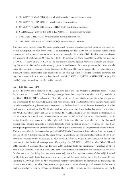
1. GARCH(1,1): GARCH(1,1) model with standard normal innovations 2. GARCH(1,1)-t: GARCH(1,1) model with t k innovations 3. GARCH(1,1)-EDF: FHS with a GARCH(1,1) conditional variance 4. EGARCH(1,1)-EDF: FHS with a EGARCH(1,1) conditional variance 5. GJR: GJR-GARCH(1,1) with standard normal innovations 6. GJR-EDF: FHS with a GJR-GARCH(1,1) conditional variance The first three models share the same conditional variance specification but differ in the distributional assumption for the error term. The remaining models allow for the leverage effect which is combined with normal errors or with errors resampled from the EDF. In this case we choose the number of replications B equal to 10000. In comparing these volatility models, we use the GARCH(1,1)-EDF and GJR-EDF as the benchmark models against which we evaluate the remaining five models. We evaluate the density, quantile and interval forecasts generated by these models using the predictive accuracy tests discussed in Section (4). In all cases, the test statistics are standard normal distributed and rejections of the null hypothesis of equal (average) accuracy for negative values indicate that the benchmark model (GARCH(1,1)-EDF or GJR-EDF) is (significantly) outperformed by the alternative model. S&P 500 Return (SP) Table (2) shows the t-statistic of the Log-Score (LS) and the Weighted Quantile Score (WQS) for h equal to 1, 2, and 5. Two findings emerge from the comparison of the volatility models to the GARCH(1,1)-EDF benchmark. First, the positive LS test statistics obtained by comparing the benchmark to the GARCH(1,1) model with normal and t distributed errors suggest that these models are significantly less accurate (compared to the benchmark) at all forecast intervals h. Similar findings are provided by the WQS with uniform weight at the 1 and 5 day horizons. In addition, the WQS statistics show that, at all horizons, the GARCH(1,1)-EDF has similar performance to the models with normal and t distributed errors on the left tail of the return distribution, but it is significantly more accurate on the right tail. It is thus the case that the three distributional assumptions provide similarly accurate forecasts when modeling negative returns, but the EDF assumption provides more precise forecasts of the right tail compared to the parametric distributions. This suggests that in the forecasting period 2000-2009 the (out-of-sample) evidence does not support the use of the t distribution for the error term. In addition, the nonparametric nature of the EDF allows to capture some asymmetry in the error distribution which is not accounted for by the parametric distributional assumptions. Comparing the GARCH(1,1)-EDF to the EGARCH and GJR models, it appears that the LS and WQS-uniform tests are significantly negative at the 1 and 2 day horizons, but only the GJR-EDF specification outperforms the benchmark for h=5. Furthermore, at the 1-day horizon we observe rejections for negative values of the WQS focused on the left and right tails, but mostly on the right tail for h=2 and at the 5-day horizon. Hence, including a leverage effect in the conditional variance specification is important in modeling the return distribution, but this effect seems less pronounced when the object of interest is the multiperiod cumulative return. When considering the GJR-EDF model as the benchmark, the Table 13
Page 1 and 2: Forecasting the Return Distribution
Page 3 and 4: the realization in addition to the
Page 5 and 6: Volatility can also experience freq
Page 7 and 8: instead let the data indicate the s
Page 9 and 10: The ultimate goal of the paper is t
Page 11: models ∆QS ij t+h (τ) = QSi t+h(
Page 15 and 16: 0.80 and 0.99 at all forecasting ho
Page 17 and 18: as a plausible benchmark. All the s
Page 19 and 20: IQR, skewness and kurtosis definiti
Page 21 and 22: References Ait-Sahalia, Y., Mykland
Page 23 and 24: Maheu, J.M. and McCurdy, T.J. (2011
Page 25 and 26: Table 2: S&P 500 Futures Return LS
Page 27 and 28: Table 4: S&P 500 Futures Return κ
Page 29 and 30: Table 6: 30-year Treasury Bond Futu
Page 31 and 32: Table 8: S&P 500 Futures Return LS
Page 33 and 34: Table 10: S&P 500 Futures Return κ
Page 35 and 36: Table 12: 30-year Treasury Bond Fut
Page 37 and 38: Table 14: 30-year Treasury Bond Fut
Page 39 and 40: Interquantile Range 95% Interval 1.
Page 41 and 42: Interquantile Range 95% Interval r

Valueat-Risk

You also want an ePaper? Increase the reach of your titles

Delete template?

Save as template?