Valueat-Risk

More documents

Recommendations

Info

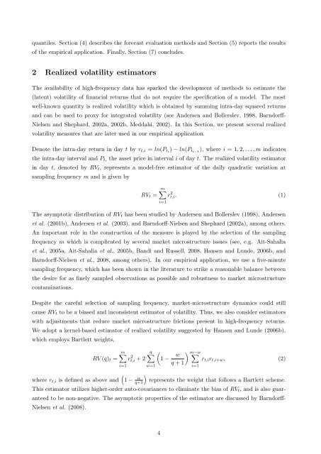
quantiles. Section (4) describes the forecast evaluation methods and Section (5) reports the results of the empirical application. Finally, Section (7) concludes. 2 Realized volatility estimators The availability of high-frequency data has sparked the development of methods to estimate the (latent) volatility of financial returns that do not require the specification of a model. The most well-known quantity is realized volatility which is obtained by summing intra-day squared returns and can be used to proxy for integrated volatility (see Andersen and Bollerslev, 1998, Barndorff- Nielsen and Shephard, 2002a, 2002b, Meddahi, 2002). In this Section, we present several realized volatility measures that are later used in our empirical application. Denote the intra-day return in day t by r t,i = ln(P ti ) − ln(P ti−1 ), where i = 1, 2, . . . , m indicates the intra-day interval and P ti the asset price in interval i of day t. The realized volatility estimator in day t, denoted by RV t , represents a model-free estimator of the daily quadratic variation at sampling frequency m and is given by m∑ RV t = rt,i. 2 (1) i=1 The asymptotic distribution of RV t has been studied by Andersen and Bollerslev (1998), Andersen et al. (2001b), Andersen et al. (2003), and Barndorff-Nielsen and Shephard (2002a), among others. An important role in the construction of the measure is played by the selection of the sampling frequency m which is complicated by several market microstructure issues (see, e.g. Ait-Sahalia et al., 2005a, Ait-Sahalia et al., 2005b, Bandi and Russell, 2008, Hansen and Lunde, 2006b, and Barndorff-Nielsen et al., 2008, among others). In our empirical application, we use a five-minute sampling frequency, which has been shown in the literature to strike a reasonable balance between the desire for as finely sampled observations as possible and robustness to market microstructure contaminations. Despite the careful selection of sampling frequency, market-microstructure dynamics could still cause RV t to be a biased and inconsistent estimator of volatility. Thus, we also consider estimators with adjustments that reduce market microstructure frictions present in high-frequency returns. We adopt a kernel-based estimator of realized volatility suggested by Hansen and Lunde (2006b), which employs Bartlett weights, m∑ q∑ ( RV (q) t = rt,i 2 + 2 1 − w ) m−w ∑ r t,i r t,i+w , (2) q + 1 i=1 w=1 i=1 ( ) where r t,i is defined as above and 1 − w q+1 represents the weight that follows a Bartlett scheme. This estimator utilizes higher-order auto-covariances to eliminate the bias of RV t , and is also guaranteed to be non-negative. The asymptotic properties of the estimator are discussed by Barndorff- Nielsen et al. (2008). 4
Volatility can also experience frequent jumps. Andersen et al. (2007) suggest that most of the predictable variation in the volatility stems from the continuous price path variability while the predictability of the jump component of volatility is typically minor. However, Wright and Zhou (2009) find that measures of realized jumps are useful predictors for bond risk premia. We follow the approach proposed by Andersen et al. (2011) to decompose the total return variability over the trading day into its continuous sample path variation and the variation due to jumps. First, we rely on the realized bipower variation measure developed by Barndorff-Nielsen and Shephard (2004), ( ) m RBV t = δ1 −2 ∑ m |r t,i ||r t,i−2 |, (3) m − 2 i=3 where δ 1 = π/2, and more generally δ η = E(|Z| η ) for Z ∼ N(0, 1). The bipower measure helps render certain types of market microstructure noise as shown by Huang and Tauchen (2005). To detect a jump, we then define the jump detection test statistics as: Z t = √(( π 2 RV t−RBV t RV t ) ( 2 + π − 5) 1 m max RT Qt 1, RBVt 2 ), (4) where ) ( ) −3 m ∑ m RT Q t = m (δ 4/3 |r t,i | 4/3 |r t,i−2 | 4/3 |r t,i−4 | 4/3 . (5) m − 4 i=5 Based on the jump detection test statistics, the realized measure of the jump contribution to the quadratic variation is then: J t = I(Z t > φ λ ) (RV t − RBV t ) , (6) where I is the indicator function and φ λ refers to an appropriate critical value from the standard normal distribution (in the empirical application we use the 99% critical level) and the continuous component of the realized measure is defined by C t = I(Z t > φ λ )RBV t + I(Z t ≤ φ λ )RV t . (7) Some markets, e.g. equity markets, are closed for a part of each 24-hour period, and the opening price on one day typically differs from the closing price on the previous day. For investors that hold their portfolios over long horizons (i.e. multiple days and beyond), the overnight return variability can directly affect their positions. Moreover, Hansen and Lunde (2006a) argue that the volatility estimator that ignores the overnight period (i.e., the market is closed) might not be a proper proxy for the true volatility. To account for the overnight return, defined as r t,0 = ln(P t,0 )−ln(P t−1,m ), we adopt the solution proposed by Blair et al. (2001) which consists of adding the squared overnight return as one of the factors in the sum of intra-day returns, that is, m∑ RV N t = rt,0 2 + RV t = rt,i. 2 (8) i=0 In the empirical application, we consider these realized volatility estimators in order to evaluate 5
Page 1 and 2: Forecasting the Return Distribution
Page 3: the realization in addition to the
Page 7 and 8: instead let the data indicate the s
Page 9 and 10: The ultimate goal of the paper is t
Page 11 and 12: models ∆QS ij t+h (τ) = QSi t+h(
Page 13 and 14: 1. GARCH(1,1): GARCH(1,1) model wit
Page 15 and 16: 0.80 and 0.99 at all forecasting ho
Page 17 and 18: as a plausible benchmark. All the s
Page 19 and 20: IQR, skewness and kurtosis definiti
Page 21 and 22: References Ait-Sahalia, Y., Mykland
Page 23 and 24: Maheu, J.M. and McCurdy, T.J. (2011
Page 25 and 26: Table 2: S&P 500 Futures Return LS
Page 27 and 28: Table 4: S&P 500 Futures Return κ
Page 29 and 30: Table 6: 30-year Treasury Bond Futu
Page 31 and 32: Table 8: S&P 500 Futures Return LS
Page 33 and 34: Table 10: S&P 500 Futures Return κ
Page 35 and 36: Table 12: 30-year Treasury Bond Fut
Page 37 and 38: Table 14: 30-year Treasury Bond Fut
Page 39 and 40: Interquantile Range 95% Interval 1.
Page 41 and 42: Interquantile Range 95% Interval r

Valueat-Risk

Create successful ePaper yourself

Delete template?

Save as template?