Matvec Users’ Guide

11.1. GENERALIZED LINEAR MODEL 77
1 5 -1 week:therapy:B
estimated value (K’b-M) = -0.86038 +- 0.323848
Prob(|t| > 2.65675) = 0.00795264 (p_value)
----------------------------------------------------------
Rate parameter
RESULTS FROM CONTRAST(S)
----------------------------------------------------------
Contrast MME_addr K_coef Raw_data_code
---------------------------------------------
1 2 1 week:intercept:1
estimated value (K’b-M) = 0.0367026 +- 0.128135
Prob(|t| > 0.286437) = 0.774573 (p_value)
----------------------------------------------------------
Finding a significantly reduced risk with drug therapy A and that the survival function did not differ
significantly from a simple exponential model.
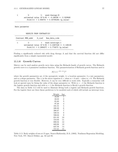
11.1.6 Growth Curves
Matvec can be used analyze growth curve data using the Richards family of growth curves. The Richards
growth curve is a 4 parameter nonlinear function. The parameterization of Richards growth function used is
A(1 ± e −b(t−t∗) ) m
where the growth parameters are A the asymptotic weight, t∗ a location parameter, b a rate parameters,
and m a shape parameter. The ± in the above equation is + when m < 0 and − when m > 0. The Richards
growth function is very flexible. However, it can be very difficult to work with. Typically a researcher will
look at special cases by fixing the value of the shape parameter m. With m = −1 the Richards function is
the logistic growth function and with m = 1 the Richards function is Brody’s growth function.
The data in Table 11.5 will be used to illustrate fitting both a logistic and Richards growth functions.
For the logistic there are three linear predictors to be modeled each of which will include an intercept term.
Weight Age
16.08 1
33.83 2
65.80 3
97.20 4
191.55 5
326.20 6
386.87 7
520.53 8
590.03 9
651.92 10
724.93 11
699.56 12
689.96 13
637.56 14
717.41 15
Table 11.5: Body weights of rats at 15 ages. Source:Ratkowsky, D.A. (1983). Nonlinear Regression Modeling.
New York, NY: Marcel Dekker, pp. 62 and 88.