Matvec Users’ Guide

84 CHAPTER 11. GENERALIZED LINEAR MIXED MODEL ANALYSES
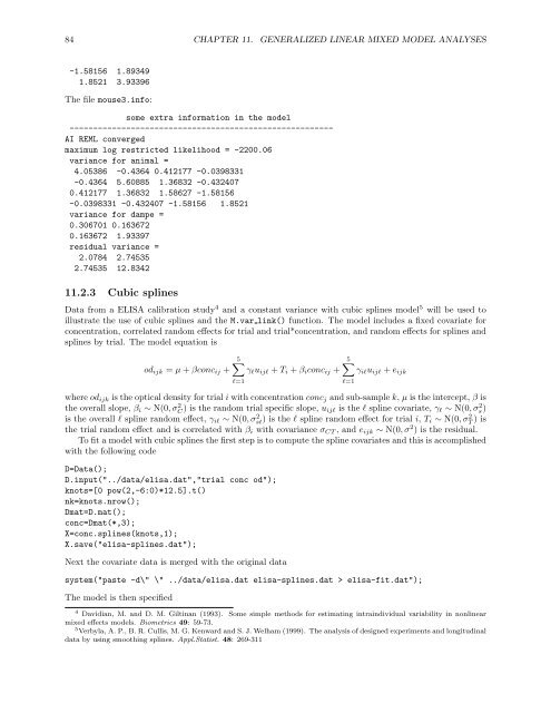
-1.58156 1.89349
1.8521 3.93396
The file mouse3.info:
some extra information in the model
--------------------------------------------------------
AI REML converged
maximum log restricted likelihood = -2200.06
variance for animal =
4.05386 -0.4364 0.412177 -0.0398331
-0.4364 5.60885 1.36832 -0.432407
0.412177 1.36832 1.58627 -1.58156
-0.0398331 -0.432407 -1.58156 1.8521
variance for dampe =
0.306701 0.163672
0.163672 1.93397
residual variance =
2.0784 2.74535
2.74535 12.8342
11.2.3 Cubic splines
Data from a ELISA calibration study 4 and a constant variance with cubic splines model 5 will be used to
illustrate the use of cubic splines and the M.var link() function. The model includes a fixed covariate for
concentration, correlated random effects for trial and trial*concentration, and random effects for splines and
splines by trial. The model equation is
od ijk = µ + βconc ij +
5∑
γ l u ijl + T i + β i conc ij +
l=1
5∑
γ il u ijl + e ijk
where od ijk is the optical density for trial i with concentration conc j and sub-sample k, µ is the intercept, β is
the overall slope, β i ∼ N(0, σ 2 C ) is the random trial specific slope, u ijl is the l spline covariate, γ l ∼ N(0, σ 2 s)
is the overall l spline random effect, γ il ∼ N(0, σ 2 st) is the l spline random effect for trial i, T i ∼ N(0, σ 2 T ) is
the trial random effect and is correlated with β i with covariance σ CT , and e ijk ∼ N(0, σ 2 ) is the residual.
To fit a model with cubic splines the first step is to compute the spline covariates and this is accomplished
with the following code
D=Data();
D.input("../data/elisa.dat","trial conc od");
knots=[0 pow(2,-6:0)*12.5].t()
nk=knots.nrow();
Dmat=D.mat();
conc=Dmat(*,3);
X=conc.splines(knots,1);
X.save("elisa-splines.dat");
Next the covariate data is merged with the original data
system("paste -d\" \" ../data/elisa.dat elisa-splines.dat > elisa-fit.dat");
The model is then specified
4 Davidian, M. and D. M. Giltinan (1993). Some simple methods for estimating intraindividual variability in nonlinear
mixed effects models. Biometrics 49: 59-73.
5 Verbyla, A. P., B. R. Cullis, M. G. Kenward and S. J. Welham (1999). The analysis of designed experiments and longitudinal
data by using smoothing splines. Appl.Statist. 48: 269-311
l=1