Weather and Climate Extremes in a Changing Climate. Regions of ...

The U.S. Climate Change Science Program Appendix A
130
Figure A.3 Density plot for the heat index data (left), and for the natural logarithms of the same data (right).
In the case under discussion, if we allow for all possible
combinations of start and finish dates, given a 111-year
series, that makes for 111x110/2=6105 tests. To apply the
Bonferroni correction in this case, we should therefore
adjust the significance level of the individual tests to
.05/6105=.0000082. However, this is still very much larger
than 10 -18 . The conclusion is that the statistically significant
result cannot be explained away as merely the result of
selecting the endpoints of the trend.
This application of the Bonferroni correction is somewhat
unusual. It is rare for a trend to be so highly significant that
selection effects can be explained away completely, as has
been shown here. Usually, we have to make a somewhat
more subjective judgment about what are suitable starting
and finishing points of the analysis.
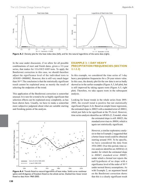
Figure A.4 Trends fitted to natural logarithms of heat index. Solid curve: nonlinear
spline with 8 degrees of freedom fitted to the whole series. Dashed line: linear trend
fitted to data from 1960-2005.
ExAMPlE 3: 1-DAY hEAVY
PRECIPITATION fREqUENCIES (SECTION
2.1.2.2)
In this example, we considered the time series of 1-day
heavy precipitation frequencies for a 20-year return value.
In this case, the density plot for the raw data is not as badly
skewed as in the earlier examples (Figure A.5, left plot), but
is still improved by taking square roots (Figure A.5, right
plot). Therefore, we take square roots in the subsequent
analysis.
Looking for linear trends in the whole series from 1895-
2005, the overall trend is positive but not statistically
significant (Figure A.6). Based on simple linear regression,
the estimated slope is .00023 with a standard error of .00012,
which just fails to be significant at the 5% level. However,
time series analysis identifies an ARMA (5, 3) model, when
the estimated slope is still .00023, the
standard error rises to .00014, which is
again not statistically significant.
However, a similar exploratory analysis
to that in Example 2 suggested that
a better linear trend could be obtained
starting around 1935. To be specific,
we have considered the data from
1934-2005. Over this period, time series
analysis identifies an ARMA(1,2)
model, for which the estimated slope
is .00067, standard error .00007,
under which a formal test rejects the
null hypothesis of no slope with a
significance level of the order of 10 -20
under normal theory assumptions. As
with Example 2, an argument based
on the Bonferroni correction shows
that this is a clearly significant result