Weather and Climate Extremes in a Changing Climate. Regions of ...

The U.S. Climate Change Science Program Appendix A
132
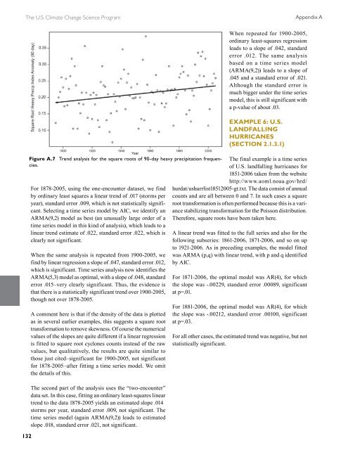
Figure A.7 Trend analysis for the square roots of 90-day heavy precipitation frequencies.
For 1878-2005, using the one-encounter dataset, we find
by ordinary least squares a linear trend of .017 (storms per
year), standard error .009, which is not statistically significant.
Selecting a time series model by AIC, we identify an
ARMA(9,2) model as best (an unusually large order of a
time series model in this kind of analysis), which leads to a
linear trend estimate of .022, standard error .022, which is
clearly not significant.
When the same analysis is repeated from 1900-2005, we
find by linear regression a slope of .047, standard error .012,
which is significant. Time series analysis now identifies the
ARMA(5,3) model as optimal, with a slope of .048, standard
error .015–very clearly significant. Thus, the evidence is
that there is a statistically significant trend over 1900-2005,
though not over 1878-2005.
A comment here is that if the density of the data is plotted
as in several earlier examples, this suggests a square root
transformation to remove skewness. Of course the numerical
values of the slopes are quite different if a linear regression
is fitted to square root cyclones counts instead of the raw
values, but qualitatively, the results are quite similar to
those just cited–significant for 1900-2005, not significant
for 1878-2005–after fitting a time series model. We omit
the details of this.
The second part of the analysis uses the “two-encounter”
data set. In this case, fitting an ordinary least-squares linear
trend to the data 1878-2005 yields an estimated slope .014
storms per year, standard error .009, not significant. The
time series model (again ARMA(9,2)) leads to estimated
slope .018, standard error .021, not significant.
When repeated for 1900-2005,
ordinary least-squares regression
leads to a slope of .042, standard
error .012. The same analysis
based on a time series model
(ARMA(9,2)) leads to a slope of
.045 and a standard error of .021.
Although the standard error is
much bigger under the time series
model, this is still significant with
a p-value of about .03.
EXAMPLE 6: U.S.
lANDfAllINg
hURRICANES
(SECTION 2.1.3.1)
The final example is a time series
of U.S. landfalling hurricanes for
1851-2006 taken from the website
http://www.aoml.noaa.gov/hrd/
hurdat/ushurrlist18512005-gt.txt. The data consist of annual
counts and are all between 0 and 7. In such cases a square
root transformation is often performed because this is a variance
stabilizing transformation for the Poisson distribution.
Therefore, square roots have been taken here.
A linear trend was fitted to the full series and also for the
following subseries: 1861-2006, 1871-2006, and so on up
to 1921-2006. As in preceding examples, the model fitted
was ARMA (p,q) with linear trend, with p and q identified
by AIC.
For 1871-2006, the optimal model was AR(4), for which
the slope was -.00229, standard error .00089, significant
at p=.01.
For 1881-2006, the optimal model was AR(4), for which
the slope was -.00212, standard error .00100, significant
at p=.03.
For all other cases, the estimated trend was negative, but not
statistically significant.