Prototyping of microfluidic systems with integrated ... - DTU Nanotech
Prototyping of microfluidic systems with integrated ... - DTU Nanotech
Prototyping of microfluidic systems with integrated ... - DTU Nanotech

Create successful ePaper yourself
Turn your PDF publications into a flip-book with our unique Google optimized e-Paper software.
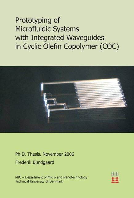
<strong>Prototyping</strong> <strong>of</strong><br />
Micr<strong>of</strong>luidic Systems<br />
<strong>with</strong> Integrated Waveguides<br />
in Cyclic Olefin Copolymer (COC)<br />
Ph.D. Thesis, November 2006<br />
Frederik Bundgaard<br />
MIC – Department <strong>of</strong> Micro and <strong>Nanotech</strong>nology<br />
Technical University <strong>of</strong> Denmark
Version as <strong>of</strong> November 7, 2006.<br />
This document contains confidential information and shall not be copied or handed<br />
over to persons not authorised by the author.
Preface<br />
This thesis is one <strong>of</strong> the requirements to fulfill in order to obtain the<br />
Ph.D. degree from the Technical University <strong>of</strong> Denmark. The work<br />
presented in this thesis has been carried out at MIC – Department<br />
<strong>of</strong> Micro and <strong>Nanotech</strong>nology between November 2003 and October<br />
2006. It has been supervised by associate pr<strong>of</strong>essor Oliver Geschke, and<br />
co-supervised by Leif Højslet Christensen <strong>of</strong> the Danish Technological<br />
Institute.<br />
The reader is invited to use both the printed and the electronic<br />
version <strong>of</strong> this document. Many <strong>of</strong> the illustrations in the thesis are<br />
in color, but an effort has gone into making all illustrations readable<br />
in black and white print nevertheless. Color prints will improve the<br />
reading experience, but a few illustrations – mostly the microscope<br />
images <strong>of</strong> the structures – are best viewed on-screen. The electronic<br />
version <strong>of</strong> the thesis is available from the homepage <strong>of</strong> the Polymeric<br />
Environmental Systems group, www.mic.dtu.dk/English/Research/<br />
BCMS/POEM at the Department <strong>of</strong> Micro and <strong>Nanotech</strong>nology, and from<br />
the author’s homepage www.nbi.dk/~bundgard. For easy navigation in<br />
the text, the PDF file has bookmarks, so that the reader can jump to<br />
the different sections <strong>of</strong> the text by clicking on the link directly in the<br />
index, or by using the bookmark pane in Adobe Reader. Also, all figure<br />
references in the text can be clicked, so that the reader is lead to the<br />
figure cited.<br />
i
Abstract<br />
In recent years, the use <strong>of</strong> polymer materials in the field <strong>of</strong> micr<strong>of</strong>luidic<br />
<strong>systems</strong> and so-called ’lab-on-a-chip’ <strong>systems</strong> has increased. Silicon,<br />
the material traditionally used for the fabrication <strong>of</strong> such <strong>systems</strong>, is<br />
not compatible <strong>with</strong> for instance blood or harsh chemicals, while many<br />
polymers have the desired properties. A number <strong>of</strong> standard polymers<br />
like poly(methyl methacrylate) and polydimethylsiloxane have been<br />
investigated, but also new polymer types <strong>with</strong> e.g. superior optical or<br />
chemical properties have emerged in micr<strong>of</strong>luidic research.<br />
The lab-on-a-chip <strong>systems</strong> integrate fluidic handling and measurement<br />
on a single chip, and both optical and electronical components can<br />
be embedded. For polymer micro<strong>systems</strong>, integration <strong>of</strong> optical waveguides<br />
can be achieved by structuring polymers <strong>with</strong> different refractive<br />
indices.<br />
This thesis treats aspects <strong>of</strong> prototyping and fabrication <strong>of</strong> micr<strong>of</strong>luidic<br />
<strong>systems</strong> in polymers, mainly in the cyclic olefin copolymer Topas.<br />
This relatively new polymer is resistant to a large number <strong>of</strong> chemicals<br />
and to strong acids, making it suited for micr<strong>of</strong>luidic <strong>systems</strong> used e.g.<br />
for long term waste water monitoring. The high refractive index and<br />
other good optical properties makes it suited for <strong>integrated</strong> optics in<br />
micr<strong>of</strong>luidic <strong>systems</strong>. Also, the engineerable glass transition temperature<br />
is an advantage, when making single-polymer <strong>systems</strong>.<br />
During the project existing fabrication methods have been adapted<br />
or improved for use <strong>with</strong> Topas, so that a number <strong>of</strong> tools for rapid<br />
prototyping <strong>of</strong> this polymer is now available. These tools include:<br />
• Micro milling <strong>of</strong> fluidic channels and optical waveguides <strong>with</strong><br />
dimensions down to 25 µm.<br />
• Spin coating <strong>of</strong> polymer layers on polymer substrates <strong>with</strong> a thickness<br />
from 100 nm to 20 µm. The spin coat layers act as a glue for<br />
ii
joining the substrate, optical layers and the lid in the micr<strong>of</strong>luidic<br />
<strong>systems</strong>.<br />
• Thermal bonding <strong>of</strong> polymer structures, including roll lamination<br />
<strong>of</strong> foil onto substrates.<br />
• Laser bonding <strong>of</strong> two polymer layers, including transparent on<br />
black, and transparent on transparent <strong>with</strong> a particle doped spin<br />
coating.<br />
• Thermal treatment <strong>of</strong> waveguides to improve the surface roughness<br />
and lower the propagation loss.<br />
The fabrication methods have been characterised, and have been<br />
optimised to minimise parameters like fabrication time, surface roughness<br />
and interface bonding strength.<br />
Using these fabrication methods, micr<strong>of</strong>luidic structures have been<br />
produced. Also, optical waveguides have been produced, exploiting the<br />
difference in refractive index <strong>of</strong> different Topas grades. Finally, optical<br />
absorption measurements have been carried out in a micr<strong>of</strong>luidic system<br />
<strong>with</strong> <strong>integrated</strong> waveguides.<br />
A demonstrator capable <strong>of</strong> distinguishing between liquids <strong>with</strong> different<br />
refractive index – in our case water and a saturated solution <strong>of</strong><br />
sugar in water – was produced using all <strong>of</strong> the techniques developed<br />
during the studies, and drawing from the knowledge about waveguides<br />
in Topas obtained in the experiments mentioned above.<br />
Finally, in a collaboration <strong>with</strong> IMTEK in Freiburg, Germany, an<br />
optical detection principle was developed. Using the principle <strong>of</strong> total<br />
internal reflection <strong>of</strong> a laser beam incident on a fluidic channel, detection<br />
<strong>of</strong> air bubbles is possible. The principle was used on a rotating platform<br />
as well as on non-moving <strong>systems</strong>.<br />
iii
Resumé<br />
Brugen af polymerer i mikr<strong>of</strong>luid-systemer, eller s˚akaldte ’lab-on-a-chip’systemer,<br />
er steget i de seneste ˚ar. Silicium, som normalt benyttes til<br />
fremstilling af disse systemer, er inkompatibelt med for eksempel blod og<br />
stærke kemikalier, hvorimod mange polymerer har de ønskede egenskaber.<br />
Flere standard-polymerer, for eksempel poly(methyl-methacrylat) og<br />
polydimethylsiloxan, er blevet undersøgt, men ogs˚a nye polymertyper<br />
med bedre optiske eller kemiske egenskaber er dukket op i mikr<strong>of</strong>luidforskningen.<br />
Lab-on-a-chip-systemer integrerer væskeh˚andtering og m˚alinger p˚a<br />
samme chip, og b˚ade optiske og elektroniske komponenter kan integreres.<br />
I mikrosystemer i polymer kan optiske bølgeledere integreres ved at<br />
strukturere polymerer med forskelligt brydningsindeks.<br />
Denne afhandling omhandler aspekter af prototyping og fabrikation<br />
af mikr<strong>of</strong>luid-systemer i polymerer, hovedsageligt i den cyclisk olefine<br />
copolymer Topas. Denne relativt nye polymer er modstandsdygtig over<br />
for mange kemikalier, blandt andet stærke syrer. Dette gør den egnet i<br />
mikr<strong>of</strong>luid-systemer til for eksempel langtidsm˚alinger af spildevand. Et<br />
højt brydningsindex og andre gode optiske egenskaber gør Topas velegnet<br />
til integrerede optiske komponenter i mikr<strong>of</strong>luid-systemer. Desuden kan<br />
glasovergangstemperaturen ændres, hvilket er en fordel ved fabrikation<br />
af systemer fremstillet i en enkelt type polymer.<br />
I løbet af projektet er eksisterende fabrikationsmetoder blevet tilpasset<br />
og optimeret til brug p˚a Topas, s˚aledes at der nu er et antal fabrikationsmetoder<br />
tilgængelige.<br />
iv
Disse metoder inkluderer:<br />
• Mikr<strong>of</strong>ræsning af væskekanaler og optiske bølgeledere med dimensioner<br />
ned til 25 µm.<br />
• Spin coating af polymer-lag p˚a polymer-substrater med lagtykkelser<br />
far 100 nm til 20 µm. Det spin coatede lag bruges som lim til at<br />
sammenføje substrat, optiske lag og l˚ag i mikr<strong>of</strong>luid-systemerne.<br />
• Termisk bonding af polymer-strukturer, blandt andet rulle-laminering<br />
af folier p˚a substrater.<br />
• Laser bonding af to polymerer, blandt andet transparent p˚a sort,<br />
og transparent p˚a transparent med et spin coated lag partikler.<br />
• Termisk efterbehandling af bølgeledere for at forbedre overfladeruheden<br />
og formindske transmissionstabet.<br />
Fremstillingsmetoderne er blevet karakteriseret, og er blevet optimeret<br />
for at minimere for eksempel fabrikationstid, overfladeruhed og<br />
maksimere eksempelvis bonding-styrke.<br />
Mikr<strong>of</strong>luid-strukturer er blevet fremstillet ved hjælp af disse metoder.<br />
Ligeledes er optiske bølgeledere blevet fremstillet ved at udnytte forskellen<br />
i brydningsindeks mellem forskellige typer Topas. Endvidere er der lavet<br />
optiske absorptionsm˚alinger i et mikr<strong>of</strong>luid-system med integrerede<br />
bøgeledere.<br />
Endelig blev en demonstrator fremstillet med de ovenst˚aende metoder,<br />
og med brug af den opbyggede viden om bølgeleder i Topas. Demonstratoren<br />
er i stand til at skelne mellem væsker med forskelligt brydningsindeks,<br />
i dette tilfælde vand og en mættet sukkeropløsning.<br />
I samarbejde med IMTEK i Freiburg, Tyskland, er et optisk detektionsprincip<br />
blevet udviklet. Ved hjælp af total intern reflektion kan<br />
en laserstr˚ale detektere luftbobler i en mikr<strong>of</strong>luid-kanal. Detektionsprincippet<br />
er blevet testet b˚ade i roterende og i stationære systemer.<br />
v
Acknowledgements<br />
Many people have helped me <strong>with</strong> a lot <strong>of</strong> things during this Ph.D.<br />
project. I am grateful to all <strong>of</strong> them.<br />
First <strong>of</strong> all, I would like to thank my supervisor, Oliver Geschke, for<br />
his help and support during the entire project. Working in the POEM<br />
group has been a pleasure, and I wish to thank all the group members<br />
and students that have been a part <strong>of</strong> the group for their inputs and<br />
help.<br />
It was a pleasure sharing my <strong>of</strong>fice <strong>with</strong> Gerardo Perozziello, and I<br />
thank him for many good discussions in Italian. Also, I thank Martin<br />
Bengtsson, Severin Dahms, and Martin F. Jensen for good roommate<br />
discussions and collaboration.<br />
I would like to thank Peter Schultz for contributing to my project<br />
<strong>with</strong> nice spin coating results.<br />
Jörg Vogel helped me out <strong>with</strong> the experimental work in the last<br />
hectic months, and contributed <strong>with</strong> a huge amount <strong>of</strong> neatly organised<br />
and easily digestible data, for which I am very thankful.<br />
I am grateful for many good hours spent <strong>with</strong> Fridolin Okkels discussing<br />
physics and life in general, and thank him for helping me out<br />
<strong>with</strong> the theoretical aspects.<br />
Thomas Anhøj helped me a lot <strong>with</strong> the optical measurements, and<br />
I am indebted to him for that.<br />
Also I would like to thank all the people at IMTEK, Freiburg for<br />
making my stay there a success, especially Thilo Brenner for being the<br />
reason for me ending up there, Jens Ducrée and Roland Zengerle for<br />
supervision, and Stefan Haeberle for good discussions.<br />
Moving to the Danish Polymer Center was facilitated by all the nice<br />
people here. I thank all for their help and for making me feel at home<br />
so quickly.<br />
vi
Many thanks to the collaborators in the µKAP center contract for<br />
their inputs to my project, including my co-supervisor Leif Højslet<br />
Christensen.<br />
Bjarne Clausen <strong>of</strong> the Department <strong>of</strong> Manufacturing Engineering<br />
and Management helped us <strong>with</strong> the bonding tests, and I thank him for<br />
that.<br />
I wish to thank Torger Tokle <strong>of</strong> COM for making his Ph.D. thesis<br />
L ATEX template public. This thesis would have looked much worse<br />
<strong>with</strong>out this input.<br />
Finally, I would like to thank all MIC and Danchip colleagues who<br />
have helped me during the project.<br />
Lyngby<br />
October 2006<br />
vii<br />
F.B.
Publications and patents<br />
The following publications have resulted from this Ph.D. project:<br />
Peer reviewed articles:<br />
[P1] Frederik Bundgaard, Gerardo Perozziello, and Oliver Geschke.<br />
Rapid prototyping tools and methods for all-Topas® cyclic olefin<br />
copolymer fluidic micro<strong>systems</strong>. Proc. IMechE Part C: Journal<br />
<strong>of</strong> Mechanical Engineering Science, 220(C11):1625-1632, 2006.<br />
[P2] Frederik Bundgaard, Jörg Vogel, and Oliver Geschke. Rapid<br />
prototyping <strong>of</strong> optical waveguides in multi-layer COC/Topas<br />
micr<strong>of</strong>luidic <strong>systems</strong>. In preparation.<br />
[P3] Gerardo Perozziello, Frederik Bundgaard, and Oliver Geschke.<br />
Fluidic Interconnections for Micr<strong>of</strong>luidic Systems: A new <strong>integrated</strong><br />
fluidic interconnection allowing plug’n’play functionality.<br />
Submitted to Sensors and Actuators.<br />
[P4] Theodor Nielsen, Daniel Nilsson, Frederik Bundgaard, Peixiong<br />
Shi, Peter Szabo, Oliver Geschke, and Anders Kristensen.<br />
Nanoimprint lithography in cyclic olefin copolymer (COC), a<br />
highly UV-transparent and chemical resistant thermoplast. Journal<br />
<strong>of</strong> Vacuum Science and Technology B, 22(4):1770–1775, 2004.<br />
Conference proceedings:<br />
[C4] Frederik Bundgaard, Gerardo Perozziello, and Oliver Geschke.<br />
Rapid prototyping methods for all-COC/Topas®Waveguides and<br />
viii
micr<strong>of</strong>luidic <strong>systems</strong>. In Klavs Jensen, Jongyoon Han, D. Jed<br />
Harrison, and Joel Voldman, editors, ”Proceedings <strong>of</strong> the µTAS<br />
2005 9th International Conference on Miniaturized Systems for<br />
Chemistry and Life Sciences”, volume 2, pages 1200–1202. The<br />
Royal Society <strong>of</strong> Chemistry, 2005.<br />
[C5] Frederik Bundgaard, Theodor Nielsen, Daniel Nilsson, Peixiong<br />
Shi, Gerardo Perozziello, Anders Kristensen, and Oliver<br />
Geschke. Cyclic Olefin Copolymer (COC/Topas®) - an exceptional<br />
material for exceptional lab-on-a-chip <strong>systems</strong>. In<br />
Thomas Laurell, Johan Nilsson, Klavs Jensen, D. Jed Harrison,<br />
and Jörg P. Kutter, editors, Proceedings <strong>of</strong> the µTAS 2004 8th<br />
International Conference on Miniaturized Systems for Chemistry<br />
and Life Sciences, volume 2, pages 372–374. The Royal Society<br />
<strong>of</strong> Chemistry, 2004.<br />
[C6] Frederik Bundgaard, Jens Ducrée, Roland Zengerle, and Oliver<br />
Geschke. <strong>Prototyping</strong> <strong>of</strong> multilayer waveguides <strong>with</strong> V-grooves in<br />
COC/Topas®. In Wolfgang Menz, Bertrand Fillon, and Stefan<br />
Dimov, editors, Proceedings <strong>of</strong> the 4M2006 Second International<br />
Conference on Multi-Material Micro Manufacture, pages 75–78.<br />
Elsevier, 2006.<br />
[C7] Frederik Bundgaard, Gerardo Perozziello, and Oliver Geschke.<br />
Rapid prototyping <strong>of</strong> all-COC/Topas® fluidic micro<strong>systems</strong>. In<br />
Wolfgang Menz and Stefan Dimov, editors, Proceedings <strong>of</strong> the<br />
4M2005 First International Conference on Multi-Material Micro<br />
Manufacture, pages 405–407. Elsevier, 2005.<br />
[C8] Frederik Bundgaard. Recent Developments in Micr<strong>of</strong>luidic<br />
Systems in Polymers. In Proceedings <strong>of</strong> Medical Plastics 2006<br />
Conference, online proceedings available on www.hexagon.dk,<br />
2006.<br />
[C9] Frederik Bundgaard. Micr<strong>of</strong>luidic Systems in Polymer Materials<br />
– Research, <strong>Prototyping</strong> and Integration. In Proceedings <strong>of</strong><br />
Medical Plastics 2005 Conference, online proceedings available<br />
on www.hexagon.dk, 2005.<br />
ix
x Publications and patents<br />
[C10] Christian Bergenst<strong>of</strong> Nielsen, Gerardo Perozziello, Frederik<br />
Bundgaard, Bjarne Helbo, P. Torben Tang, and Oliver Geschke.<br />
Micr<strong>of</strong>luidic <strong>systems</strong> in polymers performing chemical analysis.<br />
In Proceedings <strong>of</strong> Medical Plastics 2004 Conference, online proceedings<br />
available on www.hexagon.dk, 2004.<br />
[C11] Theodor Nielsen, Daniel Nilsson, Frederik Bundgaard, Peixiong<br />
Shi, Oliver Geschke, Peter Szabo, and Anders Kristensen.<br />
Nanoimprint lithography <strong>of</strong> Topas, a new thermoplast <strong>with</strong> excellent<br />
properties for lab-on-a-chip applications. In Tecnical<br />
Digest <strong>of</strong> the 48th International Conference on Electron, Ion, and<br />
Photon Beam Technology and Nan<strong>of</strong>abrication, pages 165–166,<br />
2004.<br />
[C12] Gerardo Perozziello, Martin F. Jensen, John McCormack, Frederik<br />
Bundgaard, and Oliver Geschke. Plug’n’pump fluidic interconnection.<br />
In Thomas Laurell, Johan Nilsson, Klavs Jensen,<br />
D. Jed Harrison, and Jörg P. Kutter, editors, Proceedings <strong>of</strong> the<br />
µTAS 2004 8th International Conference on Miniaturized Systems<br />
for Chemistry and Life Sciences, volume 2, pages 575–577.<br />
The Royal Society <strong>of</strong> Chemistry, 2004.<br />
[C13] O. Geschke, M. F. Jensen, F. Bundgaard, C. B. Nielsen, and<br />
L. H. Christensen. Polymer microstructures: are they applicable<br />
as optical components? In Proceedings <strong>of</strong> the SPIE - The International<br />
Society for Optical Engineering, volume 5591, page 13.<br />
2004.
Contents<br />
Preface i<br />
Abstract ii<br />
Resumé iv<br />
Acknowledgements vi<br />
Publications and patents viii<br />
Contents xi<br />
1 Introduction 1<br />
1.1 Downscaling . . . . . . . . . . . . . . . . . . . . . . . . . 2<br />
1.2 <strong>Prototyping</strong> <strong>of</strong> micr<strong>of</strong>luidic <strong>systems</strong> . . . . . . . . . . . . 4<br />
2 Theoretical aspects – micr<strong>of</strong>luidics and optics 7<br />
2.1 Introduction . . . . . . . . . . . . . . . . . . . . . . . . . 7<br />
2.2 Fluidics and micr<strong>of</strong>luidics . . . . . . . . . . . . . . . . . 8<br />
2.2.1 Mixing in micr<strong>of</strong>luidics . . . . . . . . . . . . . . . 11<br />
2.3 Waveguide optics . . . . . . . . . . . . . . . . . . . . . . 12<br />
2.3.1 Snell’s law . . . . . . . . . . . . . . . . . . . . . . 13<br />
2.3.2 Planar waveguides . . . . . . . . . . . . . . . . . 14<br />
2.3.3 Waveguide bends . . . . . . . . . . . . . . . . . . 15<br />
2.3.4 Tapered waveguides . . . . . . . . . . . . . . . . 15<br />
2.3.5 Theory and practice . . . . . . . . . . . . . . . . 17<br />
2.4 Optical measurements in micr<strong>of</strong>luidics . . . . . . . . . . 17<br />
2.4.1 Planar micr<strong>of</strong>luidics . . . . . . . . . . . . . . . . 19<br />
2.5 Summary . . . . . . . . . . . . . . . . . . . . . . . . . . 20<br />
xi
xii CONTENTS<br />
3 Polymer materials<br />
– mainly Topas 21<br />
3.1 Introduction . . . . . . . . . . . . . . . . . . . . . . . . . 21<br />
3.1.1 Why polymers? . . . . . . . . . . . . . . . . . . . 21<br />
3.2 Polymer types . . . . . . . . . . . . . . . . . . . . . . . . 23<br />
3.2.1 Thermoplastics . . . . . . . . . . . . . . . . . . . 24<br />
3.2.2 Elastomers . . . . . . . . . . . . . . . . . . . . . 25<br />
3.2.3 Thermosets . . . . . . . . . . . . . . . . . . . . . 25<br />
3.3 Polymers in micr<strong>of</strong>luidics . . . . . . . . . . . . . . . . . 26<br />
3.4 Cyclic Olefin Copolymer (COC)/Topas . . . . . . . . . . 26<br />
3.4.1 Glass transition temperature and viscosity . . . . 27<br />
3.4.2 Optical properties . . . . . . . . . . . . . . . . . 29<br />
3.4.3 Chemical resistance . . . . . . . . . . . . . . . . 30<br />
3.4.4 Injection molding and extrusion . . . . . . . . . . 32<br />
3.5 Resistance <strong>of</strong> COC to Reactive Ion Etching . . . . . . . 32<br />
3.6 Summary . . . . . . . . . . . . . . . . . . . . . . . . . . 34<br />
4 Fabrication methods 35<br />
4.1 Introduction . . . . . . . . . . . . . . . . . . . . . . . . . 35<br />
4.2 Micro milling - an introduction . . . . . . . . . . . . . . 36<br />
4.2.1 Experimental setup for micro milling . . . . . . . 38<br />
4.2.2 Experimental results . . . . . . . . . . . . . . . . 39<br />
4.3 Spin coating . . . . . . . . . . . . . . . . . . . . . . . . . 43<br />
4.4 Spin coating Topas . . . . . . . . . . . . . . . . . . . . . 44<br />
4.4.1 Spin coating Topas on Topas . . . . . . . . . . . 46<br />
4.4.2 Experimental procedure . . . . . . . . . . . . . . 47<br />
4.4.3 Results . . . . . . . . . . . . . . . . . . . . . . . 48<br />
4.4.4 A simplified mathematical model . . . . . . . . . 48<br />
4.5 Bonding and sealing <strong>of</strong> micr<strong>of</strong>luidic <strong>systems</strong> . . . . . . . 51<br />
4.6 Thermal bonding . . . . . . . . . . . . . . . . . . . . . . 52<br />
4.6.1 Thermal bonding experiments and results . . . . 53<br />
4.7 Roll lamination . . . . . . . . . . . . . . . . . . . . . . . 55<br />
4.7.1 Experiments and experimental results . . . . . . 56<br />
4.8 Laser bonding . . . . . . . . . . . . . . . . . . . . . . . . 57<br />
4.8.1 Lasers in micr<strong>of</strong>luidic manufacturing . . . . . . . 57<br />
4.8.2 Laser bonding basics . . . . . . . . . . . . . . . . 58<br />
4.8.3 Experimental results . . . . . . . . . . . . . . . . 59<br />
4.8.4 A comment on different bonding tests . . . . . . 61<br />
4.9 Summary . . . . . . . . . . . . . . . . . . . . . . . . . . 63
CONTENTS xiii<br />
5 Optical waveguides in Topas 65<br />
5.1 Waveguide fabrication . . . . . . . . . . . . . . . . . . . 66<br />
5.1.1 Spin coating and laser bonding . . . . . . . . . . 66<br />
5.1.2 Micro milling . . . . . . . . . . . . . . . . . . . . 67<br />
5.2 Propagation loss measurements . . . . . . . . . . . . . . 69<br />
5.3 Thermal treatment <strong>of</strong> the surface . . . . . . . . . . . . . 71<br />
5.3.1 A note on various methods . . . . . . . . . . . . 72<br />
5.3.2 Surface reflow using hot air . . . . . . . . . . . . 72<br />
5.3.3 Results . . . . . . . . . . . . . . . . . . . . . . . 73<br />
5.4 Optical cuvette absorbance measurements . . . . . . . . 76<br />
5.5 A refractive index sensor . . . . . . . . . . . . . . . . . . 81<br />
5.5.1 Design and fabrication . . . . . . . . . . . . . . . 81<br />
5.5.2 Experimental results . . . . . . . . . . . . . . . . 83<br />
5.5.3 Improvements . . . . . . . . . . . . . . . . . . . . 85<br />
5.6 Summary . . . . . . . . . . . . . . . . . . . . . . . . . . 85<br />
6 An opt<strong>of</strong>luidic detector 87<br />
6.1 The working principle . . . . . . . . . . . . . . . . . . . 88<br />
6.2 Experiments . . . . . . . . . . . . . . . . . . . . . . . . . 89<br />
6.2.1 Fabrication . . . . . . . . . . . . . . . . . . . . . 89<br />
6.2.2 Experimental setup . . . . . . . . . . . . . . . . . 90<br />
6.2.3 Linear scan . . . . . . . . . . . . . . . . . . . . . 90<br />
6.2.4 Rotational scan . . . . . . . . . . . . . . . . . . . 91<br />
6.3 Summary and discussion . . . . . . . . . . . . . . . . . . 94<br />
7 Discussion and outlook 95<br />
7.1 Discussion . . . . . . . . . . . . . . . . . . . . . . . . . . 95<br />
7.2 Outlook . . . . . . . . . . . . . . . . . . . . . . . . . . . 96<br />
7.2.1 Methods . . . . . . . . . . . . . . . . . . . . . . . 96<br />
7.2.2 Materials . . . . . . . . . . . . . . . . . . . . . . 97<br />
References 99<br />
A Appendix: Peer-reviewed journal papers 108
xiv CONTENTS
Chapter 1<br />
Introduction<br />
In the last two decades the field <strong>of</strong> micr<strong>of</strong>luidics and its applications<br />
have developed at an incredible pace. From the birth <strong>of</strong> the micro<br />
total analysis or µTAS concept in 1990 [1], to the status at present, a<br />
tremendous advance has been achieved in the field.<br />
Several factors were important in the creation <strong>of</strong> the µTAS field. In<br />
macroscopic chemical analysis, a chemical sample typically undergoes<br />
many different processes, such as sampling, filtering, reaction, and<br />
separation. The risk <strong>of</strong> loss and <strong>of</strong> contamination from the outside world<br />
increases for each step, along <strong>with</strong> the processing time. The time factor<br />
was also a problem when treating a large number <strong>of</strong> samples. Methods<br />
to automatise and parallelise sample treatment were requested as a<br />
solution to these problems.<br />
Flow injection analysis was invented in the mid-1970s by Ruzicka<br />
and Hansen [2]. This continuous-flow method for chemical analysis<br />
was an important step for the process <strong>of</strong> miniaturising and automating<br />
analytical chemistry.<br />
In the 1980s, the total analysis system, or TAS was conceived. The<br />
integration <strong>of</strong> all necessary processes in a single device would make the<br />
equipment bulky, and attempts to miniaturise the device were a natural<br />
consequence, leading to the coining <strong>of</strong> the µTAS concept.<br />
Soon, the term lab-on-a-chip emerged as a consequence <strong>of</strong> the fact<br />
that more than just chemical analysis could be made in such <strong>systems</strong>.<br />
Also, chemical and bio-chemical processes like synthesis and cell-culturing<br />
could potentially be made in such <strong>systems</strong>.<br />
Initially, most <strong>of</strong> the research on miniaturising chemical analysis<br />
was carried out in silicon based <strong>systems</strong>. This was caused by the fact<br />
1
2 Introduction<br />
that well-established methods were available from the semiconductor<br />
industry, where the miniaturisation <strong>of</strong> <strong>integrated</strong> circuits had been an<br />
ongoing process since the 1970s. In the last decade, however, alternative<br />
materials have been entering the µTAS scene, since both the cost and<br />
the lack <strong>of</strong> compatibility <strong>with</strong> many analytes and chemical environments<br />
make silicon a poor material choice. The interest in polymers has<br />
increased considerably, since a large variety <strong>of</strong> polymers <strong>with</strong> a diversity<br />
<strong>of</strong> properties (chemical, optical, mechanical etc.) is available at a<br />
cost considerably lower than that <strong>of</strong> silicon. Also for industrial scale<br />
production, polymers are processable <strong>with</strong> traditional low-cost methods<br />
like injection molding, which are orders <strong>of</strong> magnitude cheaper than the<br />
clean room processes used when making silicon structures.<br />
The ongoing miniaturisation in consumer electronics further increases<br />
the urge to miniaturise simple analytical <strong>systems</strong> for a number <strong>of</strong> reasons.<br />
An increased focus on and demand for the so-called point-<strong>of</strong>-care<br />
testing <strong>systems</strong> has evolved in recent years. Medical treatment can be<br />
improved if samples can be taken and analysed on-site, rather than<br />
taken to a laboratory. Since the computing power necessary for making<br />
even advanced data analysis is present today in a standard laptop<br />
computer, or even in embedded <strong>systems</strong> in hand-held analytical devices,<br />
the drive to similarly miniaturise the fluidic parts <strong>of</strong> a system is present.<br />
Miniaturising also decreases the amount <strong>of</strong> analyte and reagents needed<br />
to perform a given analysis, thus reducing the cost and environmental<br />
effects when disposing <strong>of</strong> the sample.<br />
1.1 Downscaling<br />
The question that one inevitably poses when looking at the rapid and<br />
constant miniaturisation <strong>of</strong> micr<strong>of</strong>luidic <strong>systems</strong>, is: “When is it going<br />
to end?”<br />
A number <strong>of</strong> very simple practical matters set limits in many areas<br />
<strong>of</strong> the miniaturisation. The dimensions <strong>of</strong> the human hand has set a<br />
limitation to the shrinking size <strong>of</strong> e.g. cellular phones, since the buttons<br />
must have a size comparable to the fingertip <strong>of</strong> the user for the device<br />
to work as intended.<br />
In micr<strong>of</strong>luidics, many applications can theoretically be downscaled<br />
to nan<strong>of</strong>luidics, looking at transport <strong>of</strong> single water molecules through<br />
carbon nanotubes, or similar. Here, the limit to the downscaling is the<br />
molecular scale. For many medical applications, however, the limiting
1.1 Downscaling 3<br />
Figure 1.1: Scaling <strong>of</strong> various parameters <strong>with</strong> the length scale d in a micr<strong>of</strong>luidic<br />
system. A concentration c = 1 nM <strong>of</strong> the substance to be detected, is assumed,<br />
along <strong>with</strong> a diffusion coefficient D = 10 −5 cm 2 s −1 . At the length scale <strong>of</strong> 1 µm,<br />
the reaction volume is 1 femtoliter (1 µm 3 ), which (statistically) contains one single<br />
molecule. The diffusion time is in the order <strong>of</strong> a millisecond, and the packaging density<br />
<strong>of</strong> the system is 100 million devices per square centimeter. The length scale best<br />
suited for micr<strong>of</strong>luidic devices is ∼10 – 100 µm, since enough molecules are present to<br />
yield good statistics and signal, and diffusion time is still acceptable, in the order <strong>of</strong><br />
10 seconds. Finally, some 10,000 devices per cm 2 can still be fitted onto a system.<br />
From [3], adapted from [4].<br />
factor is the size <strong>of</strong> e.g. human cells, which are in the order <strong>of</strong> 1 µm in<br />
diameter. Making micr<strong>of</strong>luidic channels smaller than the objects to pass<br />
through them would not be meaningful.<br />
Figure 1.1 shows the scaling <strong>of</strong> various parameters as a function <strong>of</strong><br />
the length scale <strong>of</strong> the micr<strong>of</strong>luidic system. One can assume a <strong>systems</strong><br />
<strong>with</strong> a concentration <strong>of</strong> 1 nM <strong>of</strong> the substance to be detected, and a<br />
diffusion constant D = 10 −5 cm 2 /s, which are typical values for small<br />
molecules, like sugar, in blood. Looking at a cube <strong>of</strong> 1 mm 3 or 1 µl <strong>of</strong><br />
liquid, the number <strong>of</strong> molecules in this volume would be in the order <strong>of</strong><br />
one billion. In the other end <strong>of</strong> the graph, a 1 µm 3 cube, <strong>with</strong> a volume<br />
<strong>of</strong> 1 femtoliter, or 10 −15 l, would – statistically – contain only one single<br />
molecule <strong>of</strong> the substance to be detected. This single molecule might<br />
even be lost in previous steps, so it is evident that the statistics are<br />
too poor to perform any reliable analysis. Also, the signal <strong>of</strong> a single
4 Introduction<br />
molecule in the detector might easily be lost in the noise <strong>of</strong> the detector<br />
electronics.<br />
The time plotted on the graph is the time it takes for a molecules<br />
to diffuse the given distance. This time is important, since the analysis<br />
result is not reliable, if the concentration unintentionally changes e.g.<br />
from the one side <strong>of</strong> a channel to the other, due to lack <strong>of</strong> time for the<br />
molecules to diffuse, and reach an equilibrium concentration throughout<br />
the entire channel width. It is seen that a molecule can diffuse 1 µm in<br />
1 ms, and that diffusion on the largest scale in the graph, 1 mm, takes<br />
in the order <strong>of</strong> 500 s or 8 minutes.<br />
The optimal size <strong>of</strong> a micr<strong>of</strong>luidic total analysis system is therefore<br />
determined by a volume big enough to yield statistically correct results,<br />
and <strong>with</strong> a number <strong>of</strong> molecules large enough to be detected by the<br />
detector system available, but small enough to make diffusion time,<br />
and thereby the time it takes to perform the analysis, short. Also, the<br />
shrinking <strong>of</strong> the system allows parallelisation <strong>of</strong> the analysis, since more<br />
units can be packaged into a given area. By comparing and evaluating<br />
the parameters listed above, the optimal system size can be found for a<br />
given application.<br />
Furthermore, the optimal size for micr<strong>of</strong>luidic <strong>systems</strong> is also determined<br />
by the manufacturing processes. Limits in terms <strong>of</strong> e.g. size,<br />
accuracy, and cost also influence heavily on the structure size in commercially<br />
available <strong>systems</strong>.<br />
Altogether, system dimensions between 10 and 100 µm seem to be<br />
the best compromise between the factors <strong>of</strong> Fig. 1.1.<br />
1.2 <strong>Prototyping</strong> <strong>of</strong> micr<strong>of</strong>luidic <strong>systems</strong><br />
The scope <strong>of</strong> the work presented in the present thesis has been to<br />
investigate, adapt and improve existing direct prototyping methods for<br />
use <strong>with</strong> the polymer Topas.<br />
Progress in metallurgy and material science in the last decade has<br />
made miniaturisation <strong>of</strong> traditional end mills down to 5 µm possible.<br />
Using high precision step motors for positioning <strong>of</strong> high speed air turbines,<br />
micro milling has become a viable method for manufacturing small<br />
quantities <strong>of</strong> structures <strong>with</strong> feature sizes down to the micrometer range.<br />
For prototyping <strong>of</strong> e.g. micr<strong>of</strong>luidic <strong>systems</strong>, this method has proven<br />
to be an alternative to standard clean room processes, due to its low
1.2 <strong>Prototyping</strong> <strong>of</strong> micr<strong>of</strong>luidic <strong>systems</strong> 5<br />
equipment costs – typically in the 10,000 e range – and the short production<br />
time.<br />
For many micr<strong>of</strong>luidic <strong>systems</strong>, a channel width and depth <strong>of</strong> 100 –<br />
200 µm is fully sufficient, and is a reasonable compromise between<br />
miniaturisation and the yield and limits <strong>of</strong> the prototyping methods.<br />
The limitations <strong>of</strong> micro milling lie in the serial nature <strong>of</strong> the manufacturing<br />
method, which impedes large-scale production, and in the<br />
accuracy and surface roughness <strong>of</strong> the finished structures. As shown in<br />
the present thesis, methods like thermal treatment, to solve or minimise<br />
these problems, exist.
Chapter 2<br />
Theoretical aspects –<br />
micr<strong>of</strong>luidics and optics<br />
2.1 Introduction<br />
<strong>Prototyping</strong> <strong>of</strong> micr<strong>of</strong>luidic system is in many ways a cross-disciplinary<br />
field. Knowledge about physics like fluid dynamics, optics, and solid<br />
state physics is required, along <strong>with</strong> chemistry – for instance knowledge<br />
about polymers and solvents – and engineering.<br />
While the design <strong>of</strong> prototypes and the development and refinement<br />
<strong>of</strong> manufacturing methods is <strong>of</strong>ten based on a combination <strong>of</strong> previous<br />
knowledge combined <strong>with</strong> intuition and a trial-and-error approach, it is<br />
still crucial to recognise the underlying physical principles and theories<br />
in play in the <strong>systems</strong>.<br />
Several theoretical issues must be considered when designing and<br />
manufacturing a micr<strong>of</strong>luidic system <strong>with</strong> <strong>integrated</strong> optical waveguides.<br />
If chemical reactions, separation, and/or mixing are to take place, it is<br />
vital that the liquid is properly mixed or separated when measurements<br />
are carried out. If, e.g., a liquid is not sufficiently well mixed when an<br />
absorbance or fluorescence measurement is carried out, erroneous results<br />
are likely to occur, since one might measure a more or less diluted part<br />
<strong>of</strong> the liquid.<br />
When designing a micr<strong>of</strong>luidic network, care must be taken to ensure<br />
that the fluid is led through the system in the proper manner. If the<br />
cross section <strong>of</strong> the micr<strong>of</strong>luidic channel is suddenly increased, e.g. by<br />
going from a channel to a larger reservoir, the drop in the pressure may<br />
generate bubbles in the system. Also, geometrical considerations are<br />
7
8 Theoretical aspects – micr<strong>of</strong>luidics and optics<br />
important when trying to avoid bubbles stuck in the system, or regions<br />
in the liquid, where recirculation takes place.<br />
If channels are split or joined the dimensions <strong>of</strong> the branches must<br />
be matched so that the right amount <strong>of</strong> liquid is lead to or from the<br />
right branches, and if a part <strong>of</strong> the liquid contains e.g. particles that<br />
are supposed to diffuse into the entire liquid, the channel width must be<br />
small enough to allow the diffusion to take place <strong>with</strong>in the length <strong>of</strong><br />
the channel.<br />
These design rules and other similar ones are taken into consideration,<br />
even when designing relatively simple structures, sometimes just as an<br />
intuitive part <strong>of</strong> the process, but sometimes also through simulations. In<br />
this manner, the properties <strong>of</strong> the structures can be tested and verified.<br />
Similarly, for the optical parts <strong>of</strong> micr<strong>of</strong>luidic system, one must<br />
recognise the underlying principles governing the system behaviour.<br />
Only then can one fully understand the possibilities and limitations <strong>of</strong><br />
the given system.<br />
In the following section, the fluidic and optical basics, and the most<br />
important principles employed in the polymer micr<strong>of</strong>luidic <strong>systems</strong> will<br />
be presented.<br />
2.2 Fluidics and micr<strong>of</strong>luidics<br />
The downscaling <strong>of</strong> <strong>systems</strong> used for transporting and analysing fluids<br />
influences the behaviour <strong>of</strong> such <strong>systems</strong>. When designing these fluidic<br />
networks, the scaling <strong>of</strong> relevant parameters will give an indication <strong>of</strong><br />
whether the system will work as desired. Some physical properties<br />
change rapidly when miniaturised, and sometimes in a not so intuitive<br />
way. Therefore, knowing the theoretical framework, and using it when<br />
designing <strong>systems</strong> is important.<br />
When designing complex <strong>systems</strong>, the use <strong>of</strong> computational fluid<br />
dynamics (CFD) is an indispensable tool. Today, numerically solving the<br />
Navier-Stokes equations has become more accessible through s<strong>of</strong>tware like<br />
ANSYS or COMSOL 1 , <strong>with</strong> special packages aimed at e.g. micr<strong>of</strong>luidics.<br />
Also, the use <strong>of</strong> new methods like topology optimisation for solving<br />
micr<strong>of</strong>luidic problems [5], is an effective way <strong>of</strong> improving the design <strong>of</strong><br />
miniaturised <strong>systems</strong>.<br />
For simpler <strong>systems</strong>, however, it is <strong>of</strong>ten sufficient to make an estimate<br />
<strong>of</strong> the key parameters to dimension the system. The parameters to keep<br />
1 Until recently, this multiphysics s<strong>of</strong>tware was know as FEMLAB.
2.2 Fluidics and micr<strong>of</strong>luidics 9<br />
in mind are listed below, <strong>with</strong> brief comments on the importance and<br />
influence on micr<strong>of</strong>luidic flows.<br />
• Viscosity. The first parameter to be introduced is the viscosity<br />
η,which is a measure <strong>of</strong> the internal friction in a liquid. It is defined<br />
as the ratio between the shear stress and the shear rate:<br />
η = F/A<br />
dv/dy<br />
(2.1)<br />
where F is the applied force, A is the area on which the force is<br />
applied, and dv/dy is the velocity gradient perpendicular to the<br />
shear direction.<br />
The viscosity is usually temperature dependent. Often viscosity<br />
is independent <strong>of</strong> the applied shear stress, like in the case <strong>of</strong> e.g.<br />
water. These liquids are called Newtonian. In non-Newtonian<br />
liquids the viscosity changes <strong>with</strong> the shear stress. Examples <strong>of</strong><br />
such liquids are shampoo and paint, which are shear-thinning, or<br />
a mixture <strong>of</strong> corn starch and water, which is shear-thickening.<br />
• Reynolds number. The second important parameter <strong>of</strong> a liquid<br />
flow is the dimension-less Reynolds number Re. Is is defined as<br />
the ratio <strong>of</strong> the inertial forces to the viscous forces, and is defined<br />
as<br />
Re = ρdv<br />
η<br />
(2.2)<br />
where ρ is the density, d is a length scale <strong>of</strong> the system (for micr<strong>of</strong>luidic<br />
channels typically the channel cross sectional dimension),<br />
and v is the flow velocity. If the inertial forces dominate, the<br />
Reynolds number is high, and the flow is said to be turbulent. In<br />
this regime, the behavior <strong>of</strong> the flow is chaotic and stochastic,<br />
meaning that a complete description is difficult, and possible only<br />
on a statistical scale.<br />
If the viscous forces dominate, the Reynolds number is low, and the<br />
flow is called laminar. Streamlines <strong>of</strong> the flow are regular and can<br />
(mostly) be calculated. Empirical observations (in macroscopic<br />
<strong>systems</strong>) have yielded a Re value <strong>of</strong> ∼2000 – 3000 as the transition<br />
between the two flow regimes.
10 Theoretical aspects – micr<strong>of</strong>luidics and optics<br />
For a typical micr<strong>of</strong>luidic channel filled <strong>with</strong> water, and <strong>with</strong> a<br />
cross sectional dimension <strong>of</strong> 100 µm and a flow speed <strong>of</strong> 1 cm/s,<br />
the Reynolds number is ∼1 at room temperature. The flow in<br />
micr<strong>of</strong>luidic channels is hence normally highly laminar. To raise<br />
the Reynolds number to the turbulent regime, a fluid velocity <strong>of</strong><br />
20 m/s would be needed. This would require a pressure difference<br />
which would probably destroy the system.<br />
• Diffusion. Often, multiple fluids or multiple concentrations <strong>of</strong> the<br />
same fluid are found in a micr<strong>of</strong>luidic system. As time passes, diffusion<br />
will minimize gradients in e.g. concentration, and smoothen<br />
out differences, so that an equilibrium is reached. This equilibrium<br />
can be a desired effect, for instance if the concentration <strong>of</strong> a<br />
substance is measured. On the other hand, if the device is sorting<br />
particles by lamination <strong>of</strong> different fluid layers, the desired state <strong>of</strong><br />
the system is as far from equilibrium as possible. The statistical<br />
movement <strong>of</strong> a single molecule in a liquid is described by the<br />
Einstein–Smoluchowski relation:<br />
x = √ 2Dt ⇔ t = x2<br />
2D<br />
(2.3)<br />
where x is the distance, D is the diffusion constant, and t is the<br />
time. The diffusion constant depends on the molecular size, and <strong>of</strong><br />
the temperature, so that small molecules diffuse faster than large<br />
ones, and the diffusion increases <strong>with</strong> the temperature.<br />
• Péclet number. The dimension-less Péclet number Pe is defined<br />
as the ratio <strong>of</strong> mass transport due to directed flow, such as that<br />
caused by a pressure gradient, to mass transport due to diffusion.<br />
It is given by the expression<br />
Pe = vd<br />
D<br />
(2.4)<br />
where v is the flow velocity, and d is a characteristic length, typically<br />
the channel width. By calculating the Péclet number, one can<br />
estimate whether the directed flow will dominate over the diffusion,<br />
or vice versa. This is important e.g. in separation processes, where<br />
a flow is split in a part <strong>with</strong> particles and a part <strong>with</strong>out. If<br />
diffusion is too high, or the flow speed is too low, particles would<br />
end up in both parts.
2.2 Fluidics and micr<strong>of</strong>luidics 11<br />
2.2.1 Mixing in micr<strong>of</strong>luidics<br />
Controlling the behaviour <strong>of</strong> the fluid in micr<strong>of</strong>luidic <strong>systems</strong> includes<br />
controlling mixing <strong>of</strong> different parts <strong>of</strong> the fluid. If the mixing <strong>of</strong> a given<br />
system is not understood or well controlled, concentration measurements<br />
might be erroneous, or separation <strong>of</strong> e.g. particles in a flow might not<br />
work as expected.<br />
As shown above, micr<strong>of</strong>luidics have low Reynolds numbers, so that<br />
turbulence in the system is excluded. The absence <strong>of</strong> turbulence, like<br />
when e.g. a cocktail is shaken, makes mixing in the system difficult,<br />
since the fluctuations in the fluid particle velocities, which are needed<br />
for turbulent mixing, are largely missing.<br />
As shown in Fig. 1.1, diffusion alone will only be sufficient for <strong>systems</strong><br />
<strong>with</strong> dimensions below a certain scale, typically some 10-100 µm, if a<br />
complete mixing <strong>of</strong> the liquid is to take place <strong>with</strong>in a reasonable time<br />
frame, that is in the order <strong>of</strong> seconds. For larger <strong>systems</strong>, <strong>with</strong> channel<br />
widths <strong>of</strong> e.g. one millimeter, diffusion time rises to many minutes,<br />
which would be too long for many point-<strong>of</strong>-care <strong>systems</strong>, and longer<br />
than when using existing, macroscopic methods.<br />
In order to mix a system efficiently, the different parts <strong>of</strong> the fluid<br />
must be rearranged. If turbulence is not achievable, as in the case <strong>of</strong><br />
micr<strong>of</strong>luidics, the fluid parts can be moved by methods like chaotic<br />
advection [6], where a liquid is mixed by repeatedly laminating and<br />
folding layers <strong>of</strong> e.g. high and low concentration. In this manner, the<br />
diffusion distance is radically reduced to the order <strong>of</strong> the single layer<br />
thickness.<br />
The stirring mechanisms used in macro-scale lamination processes can<br />
<strong>of</strong>ten only be downscaled <strong>with</strong> great difficulty to be used in micr<strong>of</strong>luidic<br />
<strong>systems</strong>. Therefore, other ways <strong>of</strong> moving liquids on this scale have been<br />
found. Mixing in the <strong>systems</strong> can be made either actively or passively. A<br />
number <strong>of</strong> elegant and effective solutions have emerged in the last decade,<br />
like the passive stacked herring-bone mixer [7, 8], where ripples split<br />
and force the flow to spiral, yielding the laminated structure. Recently,<br />
Hardt et al. have made a review <strong>of</strong> passive micromixers [9].<br />
Active devices like the cross-channel mixer [10, 11] have appeared<br />
in micr<strong>of</strong>luidics, too. Here, the interface <strong>of</strong> a two-layer fluid stream is<br />
chaotically folded and stretched by a perpendicular oscillatory motion.<br />
The benefit <strong>of</strong> active mixers is the ability to continually tune the<br />
system to achieve optimal mixing for a variety <strong>of</strong> flow velocities. For<br />
passive mixers, the mixing efficiency is <strong>of</strong>ten constrained to a limited
12 Theoretical aspects – micr<strong>of</strong>luidics and optics<br />
range in the parameter space. Contrary to the active mixers, however,<br />
no external control or actuation is needed.<br />
2.3 Waveguide optics<br />
In the last couple <strong>of</strong> decades, the continuing progress in optical waveguides<br />
research has become a key element in the development <strong>of</strong> our<br />
present society. Today, optical fibres around the world transport terabytes<br />
<strong>of</strong> information every second between all kinds <strong>of</strong> communication<br />
devices – computers, phones, faxes, radio and television, <strong>of</strong>ten from<br />
continent to continent. All the optical fibres rely on the principle <strong>of</strong> total<br />
internal reflection, where light propagates inside a dielectric material<br />
<strong>with</strong> a refractive index n1 surrounded by material <strong>with</strong> lower refractive<br />
index n2. Typically, optical fibres are made from glass, and the difference<br />
in refractive index between the core, in which the light propagates, and<br />
the cladding, is very small.<br />
Contrary to fibre optics, where the waveguide pr<strong>of</strong>ile is concentric<br />
circles, <strong>with</strong> the cladding surrounding the core, the waveguides applied<br />
in micr<strong>of</strong>luidics (and in other micro<strong>systems</strong>, for that sake) mostly have<br />
a rectangular cross section. Two examples <strong>of</strong> typical micro<strong>systems</strong><br />
waveguides are shown in Fig. 2.1, along <strong>with</strong> an optical fibre.<br />
Figure 2.1: Different optical waveguides. Left: An optical fibre. The high refractive<br />
index core is surrounded by a cladding <strong>with</strong> slightly lower refractive index. Middle:<br />
Slab or strip waveguide. The core is placed on a substrate <strong>with</strong> lower refractive index.<br />
Right: Embedded strip waveguide. The core is buried in the surrounding material.<br />
The cross sectional dimension <strong>of</strong> a waveguide determines its properties.<br />
Typical fibres used for optical communication have a core diameter<br />
<strong>of</strong> 8–10 µm, and use the near infrared part <strong>of</strong> the spectrum. Since the<br />
diameter <strong>of</strong> the core is only a few times larger than the wavelength <strong>of</strong><br />
the transmitted light, propagation can not be described by ray optics.<br />
Instead, the structure must be analysed using electromagnetic wave<br />
theory, solving Maxwell’s equations. The small size also restricts the<br />
propagation, so only one or a few electromagnetical modes can propagate<br />
in the structure [12].
2.3 Waveguide optics 13<br />
For waveguides <strong>with</strong> a cross section larger than 10 µm the propagation<br />
can be treated using ray optics. Also, a larger number <strong>of</strong> modes is allowed<br />
simultaneously in the fibre. The waveguides treated in this thesis have<br />
cross sectional dimensions in the 100–200 µm range, and are thereby<br />
clearly multi-mode fibres.<br />
2.3.1 Snell’s law<br />
When a beam <strong>of</strong> light travels from one medium to another <strong>with</strong> different<br />
refractive index, the light is refracted according to Snell’s law:<br />
n1 sin(θ1) = n2 sin(θ2) (2.5)<br />
where n1 and n2 are the refractive indices <strong>of</strong> the first and second material,<br />
respectively, and θ1 is the incoming, and θ2 the outgoing angle <strong>with</strong><br />
respect to the normal <strong>of</strong> the interface between the two materials.<br />
When moving from a dense to a less dense medium, meaning that<br />
n1 > n2, it is readily seen that no solution exists to the equation when<br />
θ1 exceeds a critical angle θc defined by<br />
n2 n1 θ 2 θ1<br />
θc = arcsin n2<br />
n1<br />
(2.6)<br />
Figure 2.2: The principle <strong>of</strong> total internal<br />
reflection. A light beam incident on<br />
an interface between a medium <strong>of</strong> refractive<br />
index n1 and a medium <strong>of</strong> refractive<br />
index n2 < n1, and entering at an angle<br />
θ1 smaller than a critical angle θc is<br />
partly refracted and partly reflected. If<br />
the incident angle exceeds the critical angle,<br />
no light is refracted. Instead, total<br />
internal reflection occurs.<br />
As illustrated in Fig. 2.2 a beam incident at an angle θ1 < θc the<br />
beam is partly reflected, and partly refracted at the interface. The larger<br />
the incident angle, the larger the part <strong>of</strong> the light which is reflected. For<br />
a beam entering at an angle θ2 > θc, no light is refracted. Instead all<br />
light undergoes total internal reflection.
14 Theoretical aspects – micr<strong>of</strong>luidics and optics<br />
2.3.2 Planar waveguides<br />
The planar waveguide principle shown in Fig. 2.3 is simple: If a ray <strong>of</strong><br />
light enters the waveguide <strong>with</strong> an angle larger than the critical angle<br />
θc, the ray will be reflected, and remain in the waveguide. The ray will<br />
propagate, since the incident angle is the same for every reflection, as<br />
long as the waveguide is straight. The ray entering at an angle θ2 smaller<br />
than the critical angle will be partly refracted out <strong>of</strong> the waveguide, and<br />
partly reflected. The refraction continues at the next point, meaning<br />
that the signal will rapidly decay.<br />
θ2 θ1 Figure 2.3: The principle <strong>of</strong> waveguiding in a planar waveguide. The ray entering at<br />
an angle θ1 larger than the critical angle θc undergo total internal reflection, while the<br />
ray entering <strong>with</strong> an angle θ2 < θc is refracted out <strong>of</strong> the waveguide. The numerical<br />
aperture NA <strong>of</strong> the optical fibre coupling the light into the waveguide must be smaller<br />
than that <strong>of</strong> the waveguide, if light is not to be coupled out at the interface.<br />
For coupling the light in and out <strong>of</strong> the waveguides, the angle <strong>of</strong><br />
the incident ray can not exceed the critical angle. For standard optical<br />
fibres <strong>with</strong> a numerical aperture NA = 0.22, this yields an exit cone<br />
angle θe <strong>of</strong> 12.7°, since<br />
NA = n sin θe<br />
n 2<br />
n 1<br />
(2.7)<br />
where n = 1 is the refractive index <strong>of</strong> air. For the step index waveguide,<br />
the numerical aperture can be defined as a function <strong>of</strong> the refractive<br />
indices <strong>of</strong> the core n1 and the cladding n2, respectively:<br />
�<br />
NA = n 2 1 − n 2 2<br />
(2.8)<br />
As shown in Chapter 5, the critical angle <strong>of</strong> the Topas system is in<br />
the order <strong>of</strong> 85°, yielding an acceptance angle <strong>of</strong> only 5°. This means<br />
that part <strong>of</strong> the light from the optical fibre is always coupled out <strong>of</strong> the<br />
system, when butt-coupling standard optical fibres to the waveguides.<br />
The system can be optimised, so that the numeric aperture <strong>of</strong> fibre<br />
and waveguide match, but this requires a change in the refractive index
2.3 Waveguide optics 15<br />
<strong>of</strong> one <strong>of</strong> the two. An other way <strong>of</strong> minimising the problem is by<br />
designing waveguide <strong>with</strong> tapered ends, so that the light is guided into<br />
the structure.<br />
2.3.3 Waveguide bends<br />
Light can propagate in a waveguide for long distances <strong>with</strong> very limited<br />
loss – for optical fibres the losses are typically measured in dB/km. The<br />
loss will, however, increase if the waveguide changes dimension, e.g. in<br />
the form <strong>of</strong> a bend. Since the incident angle will no longer be the same<br />
on both sides <strong>of</strong> the waveguide, the ray could eventually hit the sidewall<br />
at an angle smaller than the critical angle, meaning that it would be<br />
partially refracted out <strong>of</strong> the waveguide. The loss depends on the ratio<br />
between the radius <strong>of</strong> the bend R and the half-width ρ <strong>of</strong> the waveguide.<br />
In practice, the optical losses from a bend are negligible when R/ρ > 10 3 .<br />
For details, the reader is referred to e.g. [12].<br />
n 1<br />
n 2<br />
R<br />
Figure 2.4: Planar waveguide bend. The incident angle <strong>of</strong> the rays on the sidewalls<br />
change because <strong>of</strong> the bend geometry, meaning that the rays at some point could<br />
have an incident angle below the critical angle. This will lead to refraction out <strong>of</strong> the<br />
waveguide. In a planar waveguide bend, the ratio between the radius R <strong>of</strong> the bend<br />
and the half-width <strong>of</strong> the waveguide ρ is the main determinant <strong>of</strong> the optical loss in<br />
the bend. In practice, for R/ρ > 10 3 the losses are negligible. Adapted from [13].<br />
2.3.4 Tapered waveguides<br />
Waveguides can be tapered at the entry to facilitate coupling <strong>of</strong> the light<br />
into the structure. This can be an advantage in two cases, namely if<br />
ρ
16 Theoretical aspects – micr<strong>of</strong>luidics and optics<br />
the dimensions <strong>of</strong> the light source is so large that the light needs to be<br />
‘funneled’ into the waveguide, or if the alignment <strong>of</strong> the light source is<br />
difficult, meaning that a larger acceptance in angle and position <strong>of</strong> the<br />
source is needed.<br />
When designing a tapered structure for a given application, ray<br />
tracing can be used to ensure that the light is led into the waveguide<br />
from a given initial position. When considering a linear taper, as shown<br />
in Fig. 2.5, it is seen that the incident angle on the sidewalls increase for<br />
every reflection. If the taper is not designed in the proper manner, after<br />
a given number <strong>of</strong> reflections the incoming angle will no longer exceed<br />
the critical angle θc, and light will be coupled out <strong>of</strong> the waveguide.<br />
One can consider a beam entering the taper <strong>with</strong> an angle θ0. The<br />
taper has the length L, a half-width ρ0 at the entry, and a half-width<br />
ρ at the exit. For small taper angles Ω, the minimum length L <strong>of</strong> the<br />
taper can be approximated:<br />
θ 0<br />
ρ 0<br />
Lmin � (ρ0 − ρ) 2<br />
θcρ − θ0ρ0<br />
Ω<br />
L<br />
n 1<br />
n 2<br />
ρ<br />
(2.9)<br />
Figure 2.5: Waveguide taper. The ray <strong>of</strong> light is coupled into the tapered waveguide<br />
<strong>with</strong> refractive index n1, surrounded by material <strong>with</strong> refractive index n2. The side<br />
walls <strong>of</strong> the taper <strong>with</strong> length L converge at an angle Ω. The initial width is ρ0, while<br />
the width <strong>of</strong> the continuing waveguide is ρ. It is seen how the incoming angle <strong>of</strong> the<br />
ray on the sidewalls increase for every reflection. Adapted from [13].
2.4 Optical measurements in micr<strong>of</strong>luidics 17<br />
2.3.5 Theory and practice<br />
When working <strong>with</strong> prototyping methods such as micro milling, it<br />
relatively quickly becomes clear that even though all design rules have<br />
been followed, and that all the relevant calculations presented in this<br />
section have been made, the success <strong>of</strong> an experiment depends on other<br />
things.<br />
In reality, the optical losses stemming from surface roughness <strong>of</strong> the<br />
milled surfaces, random facets due to poor handling <strong>of</strong> the device and<br />
small deviations from e.g. parallel top and bottom <strong>of</strong> the waveguide, are<br />
far more significant than the theoretical losses which is predicted by the<br />
formulas.<br />
Of course, the point is that one should be aware <strong>of</strong> these principles<br />
and “good prototyping” rules, but at the same time should expect that<br />
the optical losses in the system are caused by other factors. When<br />
designing <strong>systems</strong>, one should not be afraid <strong>of</strong> deviating a bit from the<br />
principles, since optimising the manufacturing process rather than the<br />
theoretical framework will probably yield larger improvements in the<br />
results.<br />
Only when the micro manufacturing methods have improved sufficiently,<br />
and e.g. surface roughness can be minimised, so that optical<br />
surfaces <strong>with</strong> an average roughness below some 50 nm can be micro<br />
milled, the theoretical aspects will become an equally important factor<br />
in the design <strong>of</strong> <strong>systems</strong> intended for prototyping.<br />
2.4 Optical measurements in micr<strong>of</strong>luidics<br />
A variety <strong>of</strong> methods exist in analytical chemistry and biochemistry for<br />
detecting whether a given substance is present in a sample, and if so, in<br />
which quantity. Advanced, sensitive and <strong>of</strong>ten expensive methods, such<br />
as nuclear magnetic resonance (NMR), and mass spectroscopy (MS),<br />
are constantly developed and refined, and incorporate a broad range <strong>of</strong><br />
methods ranging from physics over chemistry to biochemistry.<br />
Among the most commonly used methods in chemical and biochemical<br />
measurements is a group <strong>of</strong> detection schemes all including optical<br />
sensing. It is estimated that as much as 80% <strong>of</strong> all chemical concentration<br />
measurements are carried out using these methods [14]. The optical<br />
methods include fluorescence and phosphorescence measurements, and<br />
evanescent-wave sensing. The most commonly used optical method,
18 Theoretical aspects – micr<strong>of</strong>luidics and optics<br />
I 0<br />
c,ε<br />
b<br />
I<br />
Figure 2.6: The working principle <strong>of</strong> an<br />
optical cuvette. Light <strong>with</strong> an intensity<br />
I0 is sent through the optical cuvette, containing<br />
a solution <strong>of</strong> the substance <strong>with</strong> a<br />
molar absorptivity ε and a concentration<br />
c. The light exits on the other side <strong>with</strong><br />
an intensity I.<br />
however, is the absorption detection which is carried out in order to<br />
determine the concentration <strong>of</strong> a substance in a solution. An optical<br />
cuvette is used, as shown in Fig. 2.6. Light from a laser or from a<br />
broadband light source, <strong>with</strong> intensity I0 is sent through a transparent<br />
container <strong>with</strong> an optical length b, and filled <strong>with</strong> the analyte, or a<br />
dilution <strong>of</strong> it. The solution has a concentration c and the substance has<br />
a molar absorptivity ε.<br />
On the other side, the outgoing light, now <strong>with</strong> an intensity I, is<br />
captured by an apparatus capable <strong>of</strong> measuring the intensity <strong>of</strong> the light,<br />
typically a photodiode, a photomultiplier tube (PMT), or a spectrometer.<br />
The ratio between the incoming and the outgoing intensity is called<br />
the transmittance T, and is defined as<br />
T = I<br />
The absorbance A is calculated using the relation:<br />
I0<br />
A = −log(T ) = −log I<br />
I0<br />
(2.10)<br />
(2.11)<br />
When working <strong>with</strong> optical losses in decibel, or dB, it is useful to<br />
remember the definition:<br />
� �<br />
I<br />
IdB = 10 log<br />
I0<br />
(2.12)<br />
For comparison <strong>with</strong> the absorbance A, the factor 10 must be recalled.<br />
Based on the loss in intensity, one can calculate the concentration <strong>of</strong><br />
a given solution using the empirical Lambert-Beer law:<br />
A = εbc (2.13)<br />
where A is the absorbance, ε is the molar absorptivity <strong>of</strong> the substance,<br />
b is the distance, and c is the concentration.
2.4 Optical measurements in micr<strong>of</strong>luidics 19<br />
In practice, to determine the concentration <strong>of</strong> a given substance in<br />
a sample, different pre-treatment steps like filtering, aliquoting, and<br />
chemical reactions are made, so that one is certain that the readout<br />
from the instrument really stems from the substance, and that it is not<br />
altered by the presence <strong>of</strong> other substances.<br />
Furthermore, one needs a reference measurement - typically a sample<br />
<strong>of</strong> the solvent (e.g. water or ethanol) alone, and one or several <strong>with</strong><br />
known concentrations <strong>of</strong> the substance.<br />
In micr<strong>of</strong>luidic <strong>systems</strong> the reference can be solved in the same ways<br />
as when using macroscopic instruments. Either the same optical cuvette<br />
can measure the references and the samples sequentially, or the system<br />
can be parallelised, so that multiple structures measure on the sample<br />
and references simultaneously.<br />
An elegant, commercially available example <strong>of</strong> applied optical spectroscopy<br />
is the Radiometer NPT7 blood gas analyzer [15]. Several values,<br />
like pH and pCO2, are measured on a desktop sized device using singleuse<br />
polymer cartridges <strong>with</strong> <strong>integrated</strong> optical cuvettes. By making one<br />
side <strong>of</strong> the cuvettes flexible, several hundred optical measurements in<br />
the infrared part <strong>of</strong> the spectrum can be made <strong>with</strong> different absorption<br />
lengths, meaning that the optical loss from the system can be separated<br />
from the loss stemming from the sample. In this manner, no reference<br />
measurements or calibration are needed.<br />
2.4.1 Planar micr<strong>of</strong>luidics<br />
Most micr<strong>of</strong>luidic <strong>systems</strong> today are two-dimensional or 2.5-dimensional,<br />
which roughly means that the structure can be manufactured from<br />
one side using e.g. clean room processing or micro milling. If more<br />
complicated three-dimensional structures are needed, they are usually<br />
fabricated by stacking layers <strong>of</strong> 2.5-dimensional structures. For many<br />
applications, the use <strong>of</strong> <strong>systems</strong> <strong>with</strong> a single, fixed channel depth for<br />
the entire system, is sufficient.<br />
Several methods for integrating optical detection in micr<strong>of</strong>luidics<br />
exist. The micr<strong>of</strong>luidic system can either be inserted in a macroscopic<br />
setup, where a light source shines light through a cuvette perpendicular<br />
to the micr<strong>of</strong>luidic substrate. The light is then detected by e.g. a<br />
spectrometer on the other side. Using this approach, the length <strong>of</strong><br />
the optical cuvette is defined by the thickness <strong>of</strong> the substrate, and is<br />
therefore relatively short – typically in the order <strong>of</strong> 1 mm. By coupling<br />
light into the plane <strong>of</strong> the substrate, the optical path can be prolonged
20 Theoretical aspects – micr<strong>of</strong>luidics and optics<br />
significantly. This is an advantage, since the relative error in the length<br />
decreases in this manner, and the errors <strong>of</strong> the measurements thereby<br />
are minimised accordingly.<br />
When the light is to be coupled in and out <strong>of</strong> the plane, the optical<br />
waveguides are needed. In this manner the external light source and<br />
spectrometer can be coupled to the structure using optical fibres. The<br />
waveguides then connect the optical cuvette, which can be in almost any<br />
place on the substrate, to the edges, which are accessible to the fibres.<br />
Another approach is the integration <strong>of</strong> the light source and/or detector<br />
in the micr<strong>of</strong>luidic system. If the system is silicon-based, light<br />
sources and detectors can be manufactured as a part <strong>of</strong> the structure [16].<br />
For polymer structures, the sources and detector must be manufactured<br />
separately and placed in the polymer housing. The miniaturisation <strong>of</strong><br />
light emitting diodes (LEDs) and photodiodes in recent years has made<br />
the mesoscopic solutions possible, <strong>with</strong> standard components around<br />
1 mm in size, attached to the micr<strong>of</strong>luidic system.<br />
2.5 Summary<br />
The relatively few and theoretically simple aspects treated in this chapter<br />
are meant as a basis for the practical manufacturing processes presented<br />
in the following chapters. The theory has been applied as a rough<br />
guideline to correct scaling and dimensioning <strong>of</strong> the <strong>systems</strong>. When<br />
going beyond the rapid prototyping phase, or when special effects and<br />
features are desired, one should have a more thorough look at the<br />
theoretical aspects <strong>of</strong> micr<strong>of</strong>luidics and -optics, by employing simulations<br />
and calculations to find the best solutions for a given system.<br />
For rapid prototyping using methods like micro milling, however, the<br />
single most important factor is still the manufacturing itself.
Chapter 3<br />
Polymer materials<br />
– mainly Topas<br />
3.1 Introduction<br />
When the concept <strong>of</strong> micro total analysis <strong>systems</strong> or µTAS was introduced<br />
by Manz et al. in 1990 [1], the predominanant materials used<br />
as substrates in the manufacturing <strong>of</strong> these <strong>systems</strong> were silicon and<br />
glass. The reason for this was the existence <strong>of</strong> well-developed methods<br />
for processing these materials, used in microelectronics. Here, methods<br />
like photolithography and wet etching <strong>of</strong> silicon and glass had been used<br />
and optimised for several decades. Several disadvantages when using<br />
these materials and methods for micr<strong>of</strong>luidic <strong>systems</strong> became, however,<br />
increasingly evident. This happened <strong>with</strong> the ongoing commercialisation<br />
<strong>of</strong> the technology, following the large number <strong>of</strong> developments and<br />
discoveries triggered by the introduction <strong>of</strong> the concept [17]. The search<br />
for alternative substrate materials for lab-on-a-chip <strong>systems</strong> lead to an<br />
increased focus on polymers because <strong>of</strong> several factors.<br />
3.1.1 Why polymers?<br />
Firstly, the cost <strong>of</strong> the silicon and glass is up to two orders <strong>of</strong> magnitude<br />
larger than the cost <strong>of</strong> substrates in polymers such as poly(methyl<br />
methacrylate)(PMMA) or polycarbonate (PC).<br />
Secondly, the many steps used in silicon processing, such as cleaning,<br />
wet and dry etching, resist coating, and lithographic structuring, are<br />
applied serially to each structure, thus increasing the fabrication time and<br />
21
22 Polymer materials – mainly Topas<br />
the cost. Also, even though all the processes for silicon processing have<br />
been used in large-scale production, the risk <strong>of</strong> damaging the structure<br />
increases for each process step the substrate goes through. Furthermore,<br />
many <strong>of</strong> the processes involve harmful and potentially dangerous wet<br />
chemistry like HF-etching. Using polymer as a substrate material, the<br />
fabrication cost and complexity can be significantly decreased using<br />
processes like injection moulding or hot embossing.<br />
A third limitation to the traditional processing methods are the<br />
geometrical constrictions which are imposed by the structuring methods<br />
available in standard cleanroom processing. Using isotropic chemical<br />
etching, semicircular channels can be manufactured. Dry etching is<br />
anisotropic, and structures <strong>with</strong> roughly vertical sidewalls can be created.<br />
However, the exact dimensions are <strong>of</strong>ten difficult to control, and<br />
especially structures <strong>with</strong> several different levels require many process<br />
steps, making fabrication tedious and difficult.<br />
The fourth limitation cited concerns the surface chemistry, where<br />
biomolecules <strong>of</strong>ten bond to the substrate. This is not desired in e.g.<br />
continuous flow <strong>systems</strong>, and can be avoided by surface coatings. This,<br />
however, implies yet another process step.<br />
In review articles, Becker and Gärtner [17], Soper et al. [18] and de<br />
Mello [19] list a number <strong>of</strong> properties for the ideal substrate material<br />
for micr<strong>of</strong>luidic and analytical <strong>systems</strong>, and conclude that although no<br />
single polymer <strong>of</strong>fer all the ideal properties, it is almost always possible<br />
to find a suitable polymer for a given application. The properties listed<br />
include:<br />
• Low cost <strong>of</strong> the material. This issue is even more important in micr<strong>of</strong>luidics<br />
than in e.g. microelectronics, since physical restrictions<br />
in the former make downscaling impossible <strong>with</strong>out performance<br />
loss. A 2 cm long channel used for electrophoresis cannot be fitted<br />
onto a chip shorter than 2 cm on one side <strong>with</strong>out bending the<br />
channel, and thereby decreasing the performance and the resolution<br />
<strong>of</strong> the system. Also compatibility <strong>with</strong> e.g. pipetting robots<br />
when working <strong>with</strong> microtiter plates could be an issue.<br />
• Appropriate electrical and thermal properties for the system. This<br />
is important especially in <strong>systems</strong> where electrophoresis is applied.<br />
The material must be able to <strong>with</strong>stand large electrical fields and<br />
to dissipate the Joule heat generated in the system.
3.2 Polymer types 23<br />
• Compatibility <strong>with</strong> the biological chemical substances introduced<br />
in the system, so that the system is not affected by the substances<br />
or vice versa.<br />
• Good machinability by methods such as laser ablation (infrared,<br />
ultraviolet or X-ray) or micro milling, and applicable to mass<br />
replication methods.<br />
• Good optical properties, including transparency in the visible,<br />
infrared and ultraviolet parts <strong>of</strong> the electromagnetic spectrum, so<br />
that the system can be monitored from the outside. Also, the<br />
aut<strong>of</strong>luorescence <strong>of</strong> the polymer should be limited, so that the<br />
polymer does not interfere <strong>with</strong> the light used in measurements.<br />
• Surface modification options, so that the chemical and physical<br />
properties <strong>of</strong> the polymer can be tailored to match the needs <strong>of</strong><br />
specific processes and <strong>systems</strong>.<br />
The polymers used in micr<strong>of</strong>luidic today all posses several <strong>of</strong> the properties<br />
listed above, but differ in their characteristics, such as absorption<br />
spectrum and chemical resistance. A few <strong>of</strong> the most commonly used<br />
polymers are compared in section 3.4.2.<br />
Development <strong>of</strong> polymer types <strong>with</strong> specific properties, which are<br />
tailored for specific applications in micr<strong>of</strong>luidics is not common. Contrary<br />
to industrial scale production <strong>of</strong> macroscopic objects, the polymer<br />
quantities needed for making even millions <strong>of</strong> micr<strong>of</strong>luidic structures is<br />
in the order <strong>of</strong> a few tons. This is by no means enough for a manufacturer<br />
to cover development costs, so polymers <strong>with</strong> specific features and<br />
qualities are typically still initially produced <strong>with</strong> other applications in<br />
mind, and then at a later point introduced in µTAS and micr<strong>of</strong>luidics.<br />
3.2 Polymer types<br />
It is beyond the scope <strong>of</strong> this thesis to make a general introduction to<br />
polymers and to go into details <strong>with</strong> subjects such as polymerisation and<br />
polymer chemistry. The reader is referred to e.g. [20]. However, a few<br />
remarks on key concepts relevant for micr<strong>of</strong>luidic <strong>systems</strong> are presented<br />
in this section.
24 Polymer materials – mainly Topas<br />
Traditionally, polymers are divided into three categories according to<br />
their molecular structure, namely thermoplastics which can be crystalline<br />
or non-crystalline (amorphous), elastomers also known as rubbers, and<br />
thermosets.<br />
3.2.1 Thermoplastics<br />
Thermoplastics such as PMMA, PC, polystyrene (PS), polyethylene<br />
(PE), and polyvinyl chloride (PVC) are materials that are plastic or<br />
deformable. They melt to a liquid when heated and freeze to a solid,<br />
more brittle state when cooled sufficiently. Most thermoplastics are high<br />
molecular weight polymers whose chains associate through intermolecular<br />
forces such as van der Waals or dipole-dipole forces. As the temperature<br />
is raised, these forces are overcome and the polymer chains slide between<br />
each other in the so-called rubbery state. The temperature at which<br />
the change in state happens, the glass transition temperature Tg, is not<br />
sharply defined like the freezing point for entirely crystalline substances<br />
such as water, but rather the middle <strong>of</strong> a temperature range at which<br />
the rapid change in the Young’s modulus, or elasticity, <strong>of</strong> the material<br />
happens. On a molecular level, this is the temperature at which the main<br />
polymer backbone initiates molecular motion. The Tg is controlled by<br />
cross-link density and the stiffness <strong>of</strong> the structure between cross-links.<br />
Thermoplastics can be amorphous or crystalline, or partly both. If<br />
the latter is the case, a second temperature, the melting temperature Tm<br />
is also significant for the material. At this temperature, all crystalline<br />
parts <strong>of</strong> the material have melted so only the amorphous part remains,<br />
and the polymer chains become randomly interdispersed. As the temperature<br />
increases above Tm, viscosity gradually decreases <strong>with</strong>out any<br />
distinct phase change. Generally, the amorphous parts <strong>of</strong> a polymer<br />
makes the substance more elastic, while the crystalline parts make it<br />
more stiff.<br />
At temperatures above Tg, thermoplastics can be processed by<br />
methods like injection moulding and hot embossing. The glass transition<br />
temperature can be lowered using low-molecular weight additives, or by<br />
varying the ratio between the different monomers in copolymers. In this<br />
manner, a polymer <strong>with</strong> specific properties, e.g. chemical resistance or<br />
optical properties, can to a certain extent be altered to meet fabrication<br />
requirements.
3.2 Polymer types 25<br />
3.2.2 Elastomers<br />
As indicated by the name, elastomers are deformable, elastic polymers.<br />
The polymer chains are weakly crosslinked and can be stretched to high<br />
extensions. Subsequently, the structure can revert to its original shape<br />
because <strong>of</strong> the elasticity <strong>of</strong> the material.<br />
Poly(dimethylsiloxane)(PDMS) is by far the most commonly used<br />
elastomer in micr<strong>of</strong>luidics. In the crosslinked version, where a curing<br />
agent is added to a base, it has become popular for rapid prototyping<br />
<strong>of</strong> micr<strong>of</strong>luidic devices and as a stamp material for microcontact<br />
printing. Also, hot embossing using elastomer moulds has become a<br />
popular method, and has been named s<strong>of</strong>t embossing [21, 22]. PDMS is<br />
remarkable in that it can be cast against a mould to reproduce features<br />
smaller than 100 nm. The surface free energy is low, meaning that casts<br />
release easily from moulds. Furthermore, Young’s modulus is tunable,<br />
which has led to the development <strong>of</strong> valves and pumps in microdevices<br />
using reversible deformations. A standard grade PDMS like Sylgard<br />
184 from Dow Corning is temperature stable up to 250℃, and is optically<br />
transparent well into the ultraviolet range. Some PDMS types are<br />
resistant to temperatures up to 400℃.<br />
The surface properties <strong>of</strong> PDMS can be altered using oxygen plasma<br />
treatment, which makes the surface hydrophilic. This treatment also<br />
enhances the adhesion <strong>of</strong> the surface. PDMS adheres naturally to<br />
surfaces like glass, creating non-permanent bonds which can <strong>with</strong>stand<br />
lower pressures in e.g. micr<strong>of</strong>luidic channels, while irreversible bonds<br />
are created using plasma treatment.<br />
3.2.3 Thermosets<br />
Thermosetting plastics are polymers that are cured and thereby harden.<br />
The curing happens by adding energy through heat or irradiation, or<br />
by a chemical reactions (e.g. epoxy). This leads to cross-linking <strong>of</strong> the<br />
polymer chains by covalent bonds. These bonds will not break before<br />
the rest <strong>of</strong> the polymer chain, contrary to thermoplastics where the<br />
bonds between the chains break around the glass transition temperature,<br />
while the chains remain intact.<br />
In micr<strong>of</strong>luidics, the photoresist SU-8 is an example <strong>of</strong> a thermoset.<br />
Traditionally, it is used in silicon processing as a mask layer, where UV<br />
exposure through a mask crosslinks the SU-8 in the unmasked areas.<br />
The uncured areas are then removed, and the remaining crosslinked
26 Polymer materials – mainly Topas<br />
parts are used as masks in the following etching <strong>of</strong> the silicon layer<br />
beneath.<br />
In recent years, SU-8 has been used directly for micr<strong>of</strong>luidic channels<br />
and optical waveguides using multiple layers to create more complex<br />
geometries, and for closing channels [23]. Also, sensors like cantilevers<br />
have been fabricated in SU-8 [24].<br />
3.3 Polymers in micr<strong>of</strong>luidics<br />
An ever-increasing number <strong>of</strong> polymers <strong>of</strong> all the three types listed above<br />
are being used in prototyping and manufacturing <strong>of</strong> micr<strong>of</strong>luidic <strong>systems</strong>.<br />
The requirements, such as structural stability, chemical resistance, or<br />
optical transparency, for a specific application, will limit the number <strong>of</strong><br />
polymers which are applicable in the given situation. A small number<br />
<strong>of</strong> well-known, cheap and readily available polymer materials are used<br />
in a large number <strong>of</strong> applications, especially in the prototyping phase.<br />
The advantage <strong>of</strong> using these polymers is evident: Due to the extensive<br />
documentation and experience, processing <strong>of</strong> theses polymers is less<br />
time-consuming than working <strong>with</strong> less known polymers. For a detailed<br />
comparison <strong>of</strong> these polymers, the reader is referred to [25].<br />
These commonly used polymers include PMMA, which is typically<br />
used in all-polymer-<strong>systems</strong>, where the entire system is made in the<br />
same material. Also PDMS is widely used [26–29], due to its excellent<br />
properties in the many areas listed above. PDMS <strong>systems</strong>, however, are<br />
<strong>of</strong>ten bonded on top <strong>of</strong> e.g. glass substrates due to its lack <strong>of</strong> structural<br />
stability.<br />
3.4 Cyclic Olefin Copolymer (COC)/Topas<br />
A considerable part <strong>of</strong> this thesis is centered around the cyclic olefin<br />
copolymer Topas, which is a registered trademark <strong>of</strong>, and manufactured<br />
by, Topas Advanced Polymers GmbH [30]. The reason for this fact is<br />
that Topas possesses many properties which are potentially useful in<br />
prototyping and manufacturing <strong>of</strong> micr<strong>of</strong>luidic and lab-on-a-chip <strong>systems</strong>.<br />
In this section these properties will be presented, and a comparison <strong>with</strong><br />
standard polymers like PMMA will be made.<br />
Topas is an acronym for Thermoplastic Olefin Polymer <strong>of</strong> Amorphous<br />
Structure, which is quite descriptive <strong>of</strong> the polymer in question, since<br />
Topas is an amorphous thermoplastic containing an olefin monomer (a
3.4 Cyclic Olefin Copolymer (COC)/Topas 27<br />
monomer <strong>with</strong> a double carbon-carbon bond, also known as alkene), in<br />
this case ethylene. Topas belongs among the cyclic olefin copolymers,<br />
which is a relatively new class <strong>of</strong> thermoplastics <strong>with</strong> good optical properties<br />
[31]. Apart from Topas, cyclic olefin copolymers are commercially<br />
available from a couple <strong>of</strong> manufacturers: Zeonex (Nippon Zeon, Japan),<br />
Arton (Japan Synthetic and Rubber, Japan) and Apel (Mitsui, Japan).<br />
Topas is synthesised from ethylene and cyclopentadiene, which combine<br />
to form norbonene, one <strong>of</strong> the two monomers in the copolymer,<br />
the other being ethylene. Polymerisation takes place using metallocene<br />
catalysts [32]. The structure formula <strong>of</strong> Topas is shown in Fig. 3.1.<br />
Figure 3.1: The structure formula <strong>of</strong> the cyclic olefin copolymer Topas. The two<br />
monomers are ethylene, left, and norbonene, right. The copolymer is synthesised by<br />
metallocene catalysis.<br />
3.4.1 Glass transition temperature and viscosity<br />
By varying the ratio between the two monomers the glass transition temperature<br />
can be varied from around 60℃ to above 160℃. The correlation<br />
between the norbonene content and the glass transition temperature is<br />
shown in Fig. 3.2.<br />
The four-digit data labels are the different grades <strong>of</strong> Topas numbered<br />
after two characteristic properties: The first two digits indicate the<br />
viscosity number VN which is related to the molecular weight, while<br />
the two last digit is an indication <strong>of</strong> the heat deflection temperature. An<br />
overview <strong>of</strong> the most common Topas grades is found in Table 3.1.<br />
The viscosity <strong>of</strong> the polymer is related to the length <strong>of</strong> the polymer<br />
backbone, so that longer chains will yield a higher viscosity <strong>of</strong> the<br />
substance. Intuitively, this seems right, since longer chains are more<br />
entangled <strong>with</strong> each other than shorter ones. The viscosity number indicated<br />
in the grade number is also referred to as the reduced viscosity, and<br />
is the ratio <strong>of</strong> the relative viscosity increment to the mass concentration<br />
<strong>of</strong> the polymer in a solution. It has the unit <strong>of</strong> inverse density, ml/g<br />
and is defined as:
28 Polymer materials – mainly Topas<br />
Glass transition temperature (°C)<br />
180<br />
160<br />
140<br />
120<br />
100<br />
80<br />
60<br />
40<br />
9605<br />
8007<br />
6013<br />
5013<br />
6015<br />
6017<br />
50 60 70 80 90<br />
Norbornene content (wt %)<br />
Figure 3.2: The glass transition temperature <strong>of</strong> different grades <strong>of</strong> Topas as a<br />
function <strong>of</strong> the norbonene content. A high norbonene content yields a high Tg.<br />
1<br />
VN =<br />
c( t − 1) t0<br />
(3.1)<br />
where c is the concentration <strong>of</strong> the polymer in the solvent and t and<br />
t0 are the flow times <strong>of</strong> the solution and the solvent alone, respectively.<br />
For Topas, the viscosity number is measured using a solution <strong>of</strong> 0.02%<br />
Topas in the solvent decaline at 135℃.<br />
The heat deflection temperature is the temperature at which a<br />
polymer rod <strong>of</strong> a given size is deflected irrerversibly when applying a<br />
load. Due to different test methods, the heat deflection temperature is<br />
not a well-defined parameter, but rather an indication <strong>of</strong> the highest<br />
temperature at which an injection molded structure can be removed<br />
from the tool <strong>with</strong> a deformation <strong>with</strong>in some acceptable limit. The<br />
Table 3.1: Overview <strong>of</strong> the commercially available grades <strong>of</strong> Topas, their glass<br />
transition temperature Tg and the refractive index at 633 nm. The (small) difference<br />
in n between grade 8007 and the higher Tg grades is exploited for making waveguides,<br />
as described in Chapter 2.3. Data are taken from [31].<br />
Topas grade 9506 8007 5010 5013 6013 6015 6017<br />
Tg(℃) 65 78 108 134 138 158 178<br />
Refr. index n NA 1.5361 NA 1.5319 NA 1.5320 1.5309
3.4 Cyclic Olefin Copolymer (COC)/Topas 29<br />
heat transition temperature usually lies some 5 – 10℃ below the glass<br />
transition temperature for a given material. The last two digits <strong>of</strong> the<br />
Topas grade number relate to the heat deflection temperature in the<br />
manner that the latter is approximately 10 times the two digits, meaning<br />
that Topas grade 5013 has a heat deflection temperature <strong>of</strong> 130℃.<br />
The viscosity number and the heat deflection temperature are (roughly)<br />
independent parameters. As stated above, Tg is changed by altering<br />
the norbonene content, while the viscosity – and thus the molecular<br />
weight – is changed in the polymerisation process, so that the average<br />
molecular length is altered.<br />
3.4.2 Optical properties<br />
Topas has a number <strong>of</strong> attractive optical features compared to PMMA,<br />
PC and PS. The birefringence is low, especially <strong>with</strong> high Tg grades,<br />
and it has a moderately high refractive index compared to the other<br />
polymers. The transparency is similar to that <strong>of</strong> PMMA and superior to<br />
PC and PS in the visible range. In the ultraviolet part <strong>of</strong> the spectrum,<br />
Topas is more transparent than the other polymers, as seen in Fig. 3.3.<br />
Transmission (%)<br />
100<br />
80<br />
60<br />
40<br />
20<br />
Quartz glass (Fused Silica)<br />
Topas ® 8007 X-10<br />
COC<br />
PS<br />
PC<br />
PMMA<br />
Quartz glass (Fused Silica)<br />
Glass (BK7)<br />
PMMA<br />
Glass (BK7)<br />
0<br />
180 200 220 240 260 280 300 320<br />
Wavelength (nm)<br />
340 360 380 400<br />
Figure 3.3: Ultraviolet transmission spectrum <strong>of</strong> Topas grade 8007 compared to<br />
PMMA, PC, PS and two glass types. At around 260 nm, Topas is still half transparent,<br />
contrary to the other polymer types, which are not transparent. Adapted from [33].<br />
PS<br />
PC
30 Polymer materials – mainly Topas<br />
Transmission (%)<br />
100<br />
80<br />
60<br />
40<br />
20<br />
0<br />
200 400 600 800 1000 1200 1400 1600 1800 2000<br />
Wavelength (nm)<br />
Figure 3.4: The visible and near infrared spectrum <strong>of</strong> Topas. A linear transmission<br />
is found in the visible wavelength area. The small decrease in transmission <strong>with</strong> a<br />
peak near 920 nm is found again in the waveguide measurements. Adapted from [33].<br />
The refractive index <strong>of</strong> Topas changes <strong>with</strong> the norbonene content and<br />
the glass transition temperature as seen in Fig. 3.1. Pure polyethylene<br />
has a refractive index n = 1.49 at 633 nm and low Tg Topas grade<br />
8007 has n = 1.5361, while high Tg grades have 1.5309 < n < 1.5320.<br />
This difference in refractive index between the 8007 grade and the other<br />
grades is used in the fabrication <strong>of</strong> all-Topas multilayer micr<strong>of</strong>luidic<br />
<strong>systems</strong> <strong>with</strong> <strong>integrated</strong> waveguides, as described in chapter 5.<br />
The water absorption <strong>of</strong> Topas is significantly smaller than for the<br />
other standard polymers, as seen in Table 3.2. This fact is also <strong>of</strong><br />
importance when regarding the optical properties <strong>of</strong> the polymers, since<br />
the deformation <strong>of</strong> a structure is minimised when the water absorption<br />
is small. In this manner, e.g. lens structures will deviate less from the<br />
original, dry state when exposed to water.<br />
3.4.3 Chemical resistance<br />
As stated earlier, one <strong>of</strong> the problems in fabrication <strong>of</strong> micr<strong>of</strong>luidic<br />
<strong>systems</strong> is the lack <strong>of</strong> compatibility <strong>of</strong> the structure <strong>with</strong> chemicals<br />
used in specific chemical reactions. One such incompatibility is that<br />
between ethanol, which is commonly used as solvent for many substances,<br />
and PMMA. Cracks and opacity in the structure occur <strong>with</strong>in short<br />
time, <strong>of</strong>ten leading to fluidic leakages, and making optical measurements<br />
impossible.
3.4 Cyclic Olefin Copolymer (COC)/Topas 31<br />
Table 3.2: Comparison <strong>of</strong> key material properties <strong>of</strong> Topas grade 5013 to those <strong>of</strong><br />
commonly used types <strong>of</strong> PMMA, PC and PS. It is noted that the density <strong>of</strong> Topas<br />
is 10-20% lower than that <strong>of</strong> the other polymers, and that the water absorption is<br />
significantly lower. Data are taken from [31].<br />
Value<br />
Property Topas PMMA PC PS<br />
Refractive index n (589 nm) 1.533 1.491 1.586 1.590<br />
Transmission (%), thickness 3 mm >92 >92 >89 >88<br />
Density (g/cm3 ) 1.02 1.19 1.2 1.1<br />
Heat deflection temperature<br />
(℃) at 18.2 bar<br />
120 85 120 80<br />
Water absorption (% )
32 Polymer materials – mainly Topas<br />
3.4.4 Injection molding and extrusion<br />
Since Topas became commercially available in the late 1990s, new grades<br />
have been developed constantly. The different grades shown in Table 3.1<br />
have sub-grades which are optimised for e.g. film extrusion or injection<br />
molding. Also some grades are optimised for higher UV transparency<br />
or higher optical quality than the standard grades. Even though the<br />
scope <strong>of</strong> this Ph.D. project has not been injection molding or extrusion,<br />
a number <strong>of</strong> substrates and films made by these methods have been<br />
used for this project. Using optimised process parameters and polished<br />
molds, optical quality wafers <strong>with</strong> a thickness <strong>of</strong> 1-2 mm and a surface<br />
roughness Ra <strong>of</strong> 10 nm have been produced by Teknologisk Institut <strong>with</strong><br />
whom the group has collaborated through the µKAP center contract.<br />
3.5 Resistance <strong>of</strong> COC to Reactive Ion<br />
Etching<br />
In collaboration <strong>with</strong> the Lab-on-a-chip-lasers and Nanoimprint Lithography<br />
group <strong>of</strong> MIC, a number <strong>of</strong> experiments determining the etch<br />
resistance <strong>of</strong> Topas to two different reactive ion etch processes, an oxygen<br />
plasma and an anisotropic silicon etch, has been carried out [34].<br />
The investigation, revealing some general properties <strong>of</strong> Topas, was<br />
made <strong>with</strong> nanoimprint lithography (NIL) in mind, in order to determine<br />
how suited Topas is as a substrate material for the imprint process. It<br />
is beyond the scope <strong>of</strong> this thesis to go into detail <strong>with</strong> the NIL part<br />
<strong>of</strong> the paper [34], but summarising the finding <strong>of</strong> the article, it is seen<br />
that Topas is well suited as a substrate material for thermal NIL. Silicon<br />
stamps containing nanometer as well as micrometer sized features were<br />
imprinted successfully. Furthermore, Topas was found to form completely<br />
to the stamp due to its suitable rheological properties. Finally, UVlithography<br />
on top <strong>of</strong> the Topas film patterned by NIL was demonstrated,<br />
exploiting the chemical resistance <strong>of</strong> Topas to sodium hydroxide and<br />
acetone.<br />
In the experiments concerning the reactive ion etching process, the<br />
etch resistance <strong>of</strong> Topas was compared to that <strong>of</strong> PMMA <strong>with</strong> a molecular<br />
weight <strong>of</strong> 950k (MicroChem), cross-linked SU-8 (MicroChem), and<br />
standard photoresist AZ5214E (Shipley).
3.5 Resistance <strong>of</strong> COC to Reactive Ion Etching 33<br />
Figure 3.5: Comparison <strong>of</strong> the resistance to reactive ion etching <strong>of</strong> COC/Topas<br />
to three other commonly used polymer types, namely PMMA, SU-8, and AZ5214E<br />
photoresist. Top: Etch rates using an oxygen plasma. It is seen that the etch rate <strong>of</strong><br />
Topas is comparable to that <strong>of</strong> photoresist, much better than PMMA and lower than<br />
that <strong>of</strong> crosslinked SU-8. Bottom: Using a SF6/O2 plasma, Topas is more resistant<br />
than the other polymers. The etch rates are listed in Table 3.3.<br />
14
34 Polymer materials – mainly Topas<br />
Table 3.3: Comparison <strong>of</strong> the etch rates for the four polymer types, using two<br />
different plasma types. σ is the standard deviation <strong>of</strong> the measured etch rates.<br />
O2/N2 plasma SF6/O2 plasma<br />
Substance Etch rate σ Etch rate σ<br />
(nm/s) (nm/s) (nm/s) (nm/s)<br />
PMMA 18.4 0.7 1.80 0.04<br />
Photoresist 12.1 0.2 1.00 0.02<br />
SU-8 10.2 0.4 1.04 0.02<br />
Topas 12.6 0.2 0.70 0.04<br />
First, spin coating solutions <strong>of</strong> the PMMA and Topas were prepared.<br />
A solution <strong>of</strong> 9 vol% PMMA in anisol and a 15 vol% Topas grade 5013<br />
in toluene were prepared using ultrasonication.<br />
The four different polymer solutions were spin coated onto 4-inch<br />
wafers, and cured by UV exposure and post-baking (SU-8), or by baking<br />
out the solvent from the polymer solutions (photoresist, PMMA, and<br />
Topas). Using a scalpel, a part <strong>of</strong> the spin coated layer was removed<br />
and the layer thickness was measured using a Tencor P-1 pr<strong>of</strong>ilometer.<br />
The polymers were etched using two different recipes. The first<br />
recipe gives an oxygen plasma etch and the second an anisotropic silicon<br />
etch based on a SF6/O2 plasma. The etch depth as function <strong>of</strong> time for<br />
the different polymers using the two RIE recipes are shown in Fig. 3.5.<br />
The etch rates drawn from the graphs are found in Table 3.3.<br />
3.6 Summary<br />
Topas has proven to be an interesting candidate as a material for prototyping<br />
<strong>of</strong> micr<strong>of</strong>luidic <strong>systems</strong> <strong>with</strong> <strong>integrated</strong> optical waveguides due to<br />
a number <strong>of</strong> good material properties, like high chemical resistance, and<br />
good optical properties. Compared <strong>with</strong> other thermoplastics commonly<br />
used in micr<strong>of</strong>luidics prototyping, such as PMMA and PC, Topas is<br />
superior in most aspects.<br />
The difference in refractive index between the different grades is exploited<br />
for making multi-layer Topas structures <strong>with</strong> optical waveguides<br />
in the high Tg layer. The different glass transition temperatures are also<br />
used when bonding two Topas layers.
Chapter 4<br />
Fabrication methods<br />
4.1 Introduction<br />
During this project a number <strong>of</strong> different fabrication methods for micr<strong>of</strong>luidic<br />
structures have been employed. Some <strong>of</strong> the methods are<br />
well-known from macroscopic fabrication, and have simply been scaled<br />
down to the micrometer range. Others have come from the world <strong>of</strong><br />
silicon processing, and have been developed specifically for micro and<br />
nano scale fabrication. For all the methods, however, one factor is very<br />
important, namely the accuracy.<br />
Micro milling has been investigated by a lot <strong>of</strong> research groups, and<br />
has been characterised on machines weighing several tons and taking<br />
up a small room, and yet micro milling <strong>of</strong> structures <strong>with</strong> feature sizes<br />
down to tens <strong>of</strong> micrometer is possible because <strong>of</strong> the overall accuracy<br />
<strong>of</strong> the entire system. This precision is only possible, if all parts <strong>of</strong> the<br />
milling machine are produced <strong>with</strong> very small tolerances. Also, <strong>with</strong><br />
bulky equipment, thermal expansion must be taken into consideration,<br />
since a small relative thermal expansion or contraction can result in<br />
large deviations when comparing <strong>with</strong> the size <strong>of</strong> the tools used and the<br />
structures that are produced.<br />
When spin coating substances onto substrates, the area is macroscopic,<br />
typically some 100 cm 2 . The layer thickness, on the contrary, can<br />
go down to tens <strong>of</strong> nanometer, <strong>with</strong> nanometer accuracy. For metals,<br />
sputtering devices even allow deposition <strong>of</strong> ˚Angström-thin layers.<br />
In this chapter, a general introduction will be given to the fabrication<br />
and machining methods used in the project. Also, the experiences<br />
achieved through the work will be presented and commented. The<br />
35
36 Fabrication methods<br />
results are the process parameters which have been used to successfully<br />
manufacture the components <strong>of</strong> the micr<strong>of</strong>luidic and -optical <strong>systems</strong><br />
presented in the thesis.<br />
The first section treats mechanical micro milling using a conventional<br />
computer numerical controlled (CNC) desktop sized milling machine<br />
<strong>with</strong> miniaturised tools.<br />
Secondly, an introduction will be given about spin coating <strong>of</strong> polymer<br />
solutions as a means <strong>of</strong> making thin intermittent polymer layers used in<br />
micro fabrication.<br />
Finally, the third part treats bonding <strong>of</strong> polymer micro<strong>systems</strong>,<br />
including the general principles, and the two processes thermal bonding<br />
and laser bonding.<br />
4.2 Micro milling - an introduction<br />
The continuous miniaturisation and integration <strong>of</strong> electronic circuits<br />
which has taken place during the last decades has brought along the<br />
need for high-accuracy miniaturised components, like housings and<br />
interfaces to the outer world. The demand is growing in industries like<br />
aerospace, biomedical, automotive and communications. Also, in the<br />
area <strong>of</strong> micro<strong>systems</strong> and micr<strong>of</strong>luidics, the demand for techniques and<br />
processes to bridge the gap between traditional macro- and mesoscopic<br />
components, and micro- and nanotechnology, is ever-increasing.<br />
Today, most micro-/nan<strong>of</strong>abrication is based on expensive lithographical<br />
solutions. The miniaturised traditional mechanical methods like<br />
micro-end milling do not have the same accuracy, and can not obtain as<br />
small feature sizes as when using lithography. The mechanical methods<br />
are, however, well-suited for making individual components in small<br />
quantities at a much lower price than using lithography. Contrary to<br />
many cleanroom processes, the mechanical micro-machining methods<br />
can be monitored and altered during the process, and complex threedimensional<br />
structures, which would be either impossible or extremely<br />
tedious to produce using standard clean room processing, can easily be<br />
manufactured.<br />
For fabrication <strong>of</strong> micr<strong>of</strong>luidic <strong>systems</strong>, the end-mill process is becoming<br />
increasingly popular. It is a well-known, well-established, and<br />
thoroughly investigated manufacturing process in the macroscopic world.<br />
A wide range <strong>of</strong> materials can be shaped using this method – from the
4.2 Micro milling - an introduction 37<br />
s<strong>of</strong>t and light foam-like polymers used for rapid prototyping <strong>of</strong> e.g. cars,<br />
to heavy machinery made in stainless steel.<br />
In a recent review [35], Chae et al. made a survey <strong>of</strong> the state-<strong>of</strong>-theart<br />
in micro-mechanical machining research. They list the issues which<br />
have been or are currently being addressed by the research community,<br />
and the challenges connected <strong>with</strong> the miniaturisation <strong>of</strong> mechanical<br />
milling processes.<br />
The improvements in the fabrication methods for micro-tools in<br />
tungsten carbide, using e.g. vibration grinding and focused ion beam,<br />
has diminished the minimum tool diameter significantly in the last<br />
decade. End mills <strong>with</strong> a diameter down to 25 µm are now commercially<br />
available, e.g. by Performance Micro Tool [36] at a price <strong>of</strong> around 50 e.<br />
A reason for this development is the improvement in metallurgy and<br />
the understanding <strong>of</strong> e.g. grain size and chemical composition on the<br />
hardness and the wear resistance <strong>of</strong> the tools. Manufacturing <strong>of</strong> carbide<br />
tools can be made using focused ion beam (FIB) [37].<br />
However, durability and accuracy <strong>of</strong> the tools is still an issue, especially<br />
because it is still difficult to detect dimensional changes on the<br />
tools. A not uncommon problem in micro milling is to detect whether<br />
the tool is intact, or whether one, indeed, is milling <strong>with</strong>out the flutes,<br />
but simply using the remains <strong>of</strong> the shaft.<br />
The wear on the tools is to a great extent caused by the fact that<br />
the accuracy <strong>of</strong> the macroscopic machinery attached to the micro-tool<br />
has not been improved and downscaled accordingly. It is not uncommon<br />
that the run-out, or eccentricity, <strong>of</strong> a spindle is in the order <strong>of</strong>, or even<br />
larger than, the diameter <strong>of</strong> the tool. This causes a far greater stress on<br />
the tool, than if the tool was rotating around its own axis.<br />
One solution to this problem are the so-called micro factories, where<br />
all components are scaled down [38, 39]. In this manner an entire<br />
workshop, containing miniaturised lathe, micro mill and micro press is<br />
contained in a brief case sized housing. Using less much raw material, the<br />
quality and precision <strong>of</strong> the materials used can be improved, and better<br />
quality machines can be built for the same price. Typically actuation <strong>of</strong><br />
the XY stage is piezo-electric rather than spindle-based as on normal<br />
milling machines.<br />
Significantly higher cutting speeds can be obtained, due to the<br />
diminished mass <strong>of</strong> the movable parts in the spindle. This improves the<br />
quality <strong>of</strong> the cutting.
38 Fabrication methods<br />
An impressive example <strong>of</strong> a downscaled, custom built system <strong>with</strong><br />
extreme accuracy is the 5-axis micro milling machine built by Bang<br />
et al. [40]. Using a high speed spindle and translational stages <strong>with</strong><br />
50 nm resolution, micro milled structures are produced in brass, <strong>with</strong> a<br />
footprint <strong>of</strong> 50 µm × 50 µm and a height <strong>of</strong> more than 500 µm, i.e. an<br />
aspect ratio over 10. A cylindrical structure 30 µm in diameter <strong>with</strong> an<br />
aspect ratio <strong>of</strong> 21.6 was also produced.<br />
The mechanism <strong>of</strong> micro-scale chip formation is another area which<br />
has not yet been understood fully. A minimum chip thickness exists,<br />
below which the material is not cut, but elastically deformed. In macroscale<br />
milling, the edge radius <strong>of</strong> the tool is usually negligible compared<br />
to the chip thickness, but in micro milling, the radius <strong>of</strong> the tool edge is<br />
<strong>of</strong>ten comparable to the chip dimension, and known theoretical models<br />
fail. Therefore, predicting the minimum chip thickness is still difficult<br />
in micro milling. Similarly, measuring the cutting forces is extremely<br />
difficult.<br />
Burr formation and minimisation there<strong>of</strong> is another important issue<br />
in micro milling. Lee and Dornfeld [41] have investigated which factors<br />
influence the creation <strong>of</strong> burrs during micro milling. The tool wear, the<br />
feed per tooth, and the cutting speed are important factors.<br />
Generally, most <strong>of</strong> the micro milling investigations have been carried<br />
out on steel or other metal, while micro milling <strong>of</strong> polymers is largely<br />
absent in the literature. Furthermore, since material parameters like<br />
elasticity and glass transition temperature vary a lot from polymer to<br />
polymer, all process parameters must be optimised for the single polymer<br />
type.<br />
4.2.1 Experimental setup for micro milling<br />
For the experiments presented in this thesis, a commercially available<br />
desktop milling machine was used. Figure 4.1 shows the Mini-Mill/3PRO<br />
from Minitech [42]. It is a computer controlled three-axis system <strong>with</strong><br />
a NSK EM-501 50,000 rpm electrical spindle [43]. The step motors<br />
controlling the stage employ micro-stepping, and a XYZ resolution <strong>of</strong><br />
around 1 µm is achieved. The repeatability <strong>of</strong> the system, including the<br />
spindle run-out, is less than 5 µm.<br />
The structures to be milled were designed using the commercial<br />
CAD s<strong>of</strong>tware Rhino [44] <strong>with</strong> the RhinoCAM [45] plug-in. The milling<br />
machine is controlled by Mach3 [46] s<strong>of</strong>tware.
4.2 Micro milling - an introduction 39<br />
a<br />
b<br />
200 µm<br />
Figure 4.1: a. The micro milling machine, Mini.Mill/3 PRO from Minitech Machinery.<br />
The 50,000 rpm spindle is electrical. b. Microscope image <strong>of</strong> micro milling tools<br />
<strong>with</strong> diameters <strong>of</strong> 200 µm and 25 µm, respectively.<br />
4.2.2 Experimental results<br />
An investigation <strong>of</strong> milling parameters using a 200 µm end mill on Topas<br />
grades 5013 and 8007 was carried out, in order to determine the feed<br />
speed and rotational speed yielding the best surface roughness. A limited<br />
number <strong>of</strong> feed speeds and rotational speeds was investigated, based on<br />
previous experiences. Fig. 4.2 show the average surface roughness Ra<br />
measured using a Dektak 8 pr<strong>of</strong>ilometer <strong>with</strong> a 5 µm stylus. It is seen<br />
that Ra on average lies around 100 nm; however, this does not take into<br />
account the waviness <strong>of</strong> the structure. It is seen that a higher rotational<br />
speed seems to give a lower average roughness. Still, the wear <strong>of</strong> the tool<br />
and the run-out <strong>of</strong> the spindle can be much more important than the<br />
factors investigated. The average roughness <strong>of</strong> the milled structures is<br />
an order <strong>of</strong> magnitude larger than that <strong>of</strong> the surface <strong>of</strong> the substrates,<br />
which is ∼9 nm.<br />
Other than the surface roughness <strong>of</strong> the structures, the minimisation<br />
<strong>of</strong> the creation <strong>of</strong> burrs was an important issue. Usually, there is<br />
a difference in the amount <strong>of</strong> burr deposited, depending on whether
40 Fabrication methods<br />
Average roughness Ra (nm)<br />
250<br />
200<br />
150<br />
100<br />
50<br />
0<br />
30k RPM grade 5013<br />
50k RPM grade 5013<br />
30k RPM grade 8007<br />
50k RPM grade 8007<br />
0 10 20 30 40 50 60<br />
Feed speed (mm/min)<br />
Figure 4.2: Surface roughness Ra <strong>of</strong> micro milled structures using a 200 µm tool on<br />
Topas grades 5013 and 8007. The surface roughness is plotted as a function <strong>of</strong> the<br />
feed speed and the rotational speed <strong>of</strong> the spindle. A higher rotational speed seems<br />
to yield a lower surface roughness.<br />
conventional or climb milling 1 , is used. For micro milling it seems to<br />
be more complicated to determine which method is the better, and the<br />
result varies <strong>with</strong> the material, speeds and tool size.<br />
Micro milled metal structures, and structures in PMMA can be<br />
polished using various commercially available methods like polishing<br />
pastes or fine grain sand paper, and optical surfaces are achievable.<br />
For Topas, mechanical polishing has proven somewhat more difficult.<br />
The reason for this is the relatively s<strong>of</strong>t burrs, especially for the grade<br />
8007. Using ultrasonication, some burrs can be removed, but the result<br />
depends on the burr size. Larger burrs can usually only be removed<br />
mechanically.<br />
For the micro milled waveguide structures presented later in this<br />
thesis, it was also important to minimise the manual polishing and<br />
de-burring, since this would increase the geometrical differences between<br />
the structures. In this manner, when measuring optical losses, it would<br />
be impossible to separate the intrinsic loss <strong>of</strong> the waveguide from the<br />
extra loss caused by scratches and the like, produced during de-burring.<br />
The optimised milling parameters for the waveguides produced <strong>with</strong><br />
500 µm end mills, and presented in Chapter 5, are 20,000 rpm and a<br />
1 In conventional milling, the feed direction and the rotational direction at the<br />
cutting site are pointing in the same direction. In climb milling, the feed is opposed<br />
to the rotational direction.
4.2 Micro milling - an introduction 41<br />
500 µm<br />
Figure 4.3: The importance <strong>of</strong> optimising milling parameters. Top. A 200 µm wide<br />
and 250 µm deep waveguide milled in Topas grade 5013 <strong>with</strong> a 500 µm end mill using<br />
non-optimised parameters. Bottom. The same structure milled <strong>with</strong> the same tool,<br />
but using optimised parameters. A significant decrease in burr is seen.<br />
feed speed <strong>of</strong> 110 mm/min using conventional milling. As seen, the<br />
rotational speed is lower than for the 200 µm tools, but the feed speed<br />
is higher. An example <strong>of</strong> a waveguide structure milled <strong>with</strong> the 50 µm<br />
tool using non-optimised and optimised parameters is shown in Fig. 4.3.<br />
The fact that a lower speed yield a better result could a priori seem<br />
contradictive to most results saying that the higher rotational speed, the<br />
better. This assumption, however, mostly relates to milling <strong>of</strong> metals.<br />
For polymers, the fact that the material can melt relatively easily, if care<br />
is not taken to sufficiently cool the system, will <strong>of</strong>ten set a maximum<br />
rotational speed which is far lower than the rotational speed used for<br />
metals.<br />
Figure 4.4 shows various micr<strong>of</strong>luidic structures, all micro milled in<br />
Topas. The channel dimensions vary from 200 µm down to 25 µm.
42 Fabrication methods<br />
a b<br />
c d<br />
e<br />
1mm<br />
200 µm<br />
3mm 0.5 mm<br />
f<br />
1mm<br />
100 µm<br />
Figure 4.4: Various micro milled structures in Topas. a. Scanning Electron<br />
Microscope (SEM) image <strong>of</strong> a micro milled meander structure. The channels are<br />
100 µm wide and deep, and the through-holes are 500 µm in diameter. b. Closeup<br />
<strong>of</strong> the meander. c. SEM image <strong>of</strong> a micro milled system <strong>with</strong> 200 µm wide and<br />
deep channels (left) and 25 µm wide and deep channels (middle and right). The<br />
through-holes are 300 µm in diameter. d. Optical microscope image <strong>of</strong> a similar<br />
structure <strong>with</strong> 200 µm and 25 µm channels. e. T-junction made <strong>with</strong> 100 µm wide<br />
and deep channels. A lid has been laser bonded on the structure to seal it. Blue<br />
liquid has been put into the system for visual enhancement. Inset: Closeup <strong>of</strong> the<br />
junction. f. Two 25 µm meander structures compared to a human hair.
4.3 Spin coating 43<br />
4.3 Spin coating<br />
A much used method for adding thin layers <strong>of</strong> material on top <strong>of</strong> e.g.<br />
silicon wafers is spin coating. Photoresists and other mask materials<br />
can be applied <strong>with</strong> an accuracy <strong>of</strong> a few micrometers in thickness, and<br />
<strong>with</strong> thicknesses spanning many orders <strong>of</strong> magnitude; from nanometer<br />
to hundreds <strong>of</strong> micrometer thick layers. Two key parameters can be<br />
varied to obtain the right layer thickness:<br />
The viscosity <strong>of</strong> the fluid can be varied. Usually, the fluid is a<br />
solution <strong>of</strong> e.g. a polymer and a solvent, where the latter evaporates,<br />
partly during the spin coating process, and partly during the subsequent<br />
post-baking, or annealing. By varying the ratio between solute and<br />
solvent, the viscosity <strong>of</strong> the solution is readily changed.<br />
The rotational speed also influences the thickness <strong>of</strong> the final layer,<br />
so that a higher speed yields a thinner layer.<br />
The substrate to be coated is usually circular and is placed on a chuck<br />
connected to a motor in the spin coating device, so that the substrate can<br />
rotate. Typical rotational speeds lie from 500 rpm 5,000 rpm. Usually,<br />
the substrate is held in place by vacuum. Care must be taken to center<br />
the substrate sufficiently, since an eccentrically placed substrate rotating<br />
at high speed can detach from the vacuum chuck if the forces are<br />
adequately large. Also, the eccentricity can lead to uneven spin coated<br />
layers, caused by vibrations in the substrate when not properly aligned.<br />
The theoretical thickness <strong>of</strong> a spin coated layer <strong>of</strong> a given solution<br />
can be calculated using the formula below, taken from [47].<br />
T = K · Cβ · ηγ ωα (4.1)<br />
where T is the thickness <strong>of</strong> the spin coated layer, C is the concentration<br />
<strong>of</strong> polymer in g/ml, η is the intrinsic viscosity <strong>of</strong> the polymer, ω is the<br />
rotational speed in rotations/minute, and K, α, β and γ are constants.<br />
This expression tells that high concentration, high intrinsic viscosity<br />
and low rotational speed will give a thick layer, while low polymer<br />
concentration, low viscosity and high rotational speed will yield a thinner<br />
layer.
44 Fabrication methods<br />
Generally, the spin coating process can be divided into four phases<br />
[48]:<br />
• First, the solution is deposited on the wafer. A nozzle (for permanent<br />
<strong>systems</strong>) or a pipette (when applying the solution manually)<br />
is placed at the center <strong>of</strong> the substrate, typically some 1-3 centimeters<br />
above it. Either the solution as applied on a non-rotating<br />
substrate, or the substrate is set in rotation at a low angular velocity,<br />
typically around 500-800 rpm. Then a quantity <strong>of</strong> solution,<br />
typically a few milliliter, is poured onto the rotating substrate.<br />
Care must be taken to make the process smooth and continuous,<br />
<strong>with</strong> as few drops and splashes as possible. In this manner, the<br />
quality <strong>of</strong> the spin coated layer is maximised.<br />
• The substrate is now accelerated to a fixed rotational speed, and<br />
the solution spreads over the entire substrate. A large quantity <strong>of</strong><br />
the liquid is ejected from the edge <strong>of</strong> the disk. Initially, vortices<br />
may form due to the inertia <strong>of</strong> the top layers <strong>of</strong> the fluid, but<br />
rapidly, all fluid remaining on the substrate co-rotates.<br />
• In the third phase, the fluid is gradually thinned. This process is<br />
dominated by the viscous forces <strong>of</strong> the fluid. At the edge, beads<br />
are <strong>of</strong>ten seen, and thickness variations are common.<br />
• The fourth phase is dominated by the evaporation <strong>of</strong> the solvent.<br />
The viscous thinning <strong>of</strong> the fluid and the evaporation occur simultaneously,<br />
but the processes dominate at different points during<br />
the spin coating process. When the evaporation becomes the most<br />
important process, the solution will thicken and eventually become<br />
gel-like. For a more in-depth description, the reader is referred<br />
to [49].<br />
4.4 Spin coating Topas<br />
The theoretical considerations are also valid for spin coating <strong>of</strong> Topas<br />
on silicon substrates, and publications including investigations <strong>of</strong> spin<br />
coated Topas layers for nanoimprint lithography have been published in<br />
recent years, e.g. [50].<br />
A major issue in the investigations has been the surface roughness<br />
<strong>of</strong> the spin coated layer. For end processes like nanoimprint lithography,
4.4 Spin coating Topas 45<br />
the surface roughness must be low, typically below 40 nm. This has<br />
proven to be a problem, and efforts have gone into improving the surface<br />
quality.<br />
When spin coating different solutions <strong>of</strong> Topas dissolved in toluene<br />
onto substrates, it was seen that it was difficult to get smooth and homogeneous<br />
layers. The problem seemed to be that the toluene evaporated<br />
too quickly, so that initial inhomogeneities stemming from the process<br />
<strong>of</strong> pouring the solution onto the substrate did not disappear during the<br />
later processing steps. This can be accounted for by the fact that the<br />
evaporation from thin areas takes place more rapidly than from thicker<br />
areas. The thin areas become gel-like and the liquid can not flow to<br />
level out, leaving the thicker areas confined.<br />
Bilenberg et al. [50] solved the problem <strong>of</strong> surface roughness by<br />
imprinting an blank silicon wafer onto the spin coated layer to smoothen<br />
out any roughness or defect. In this manner, a surface roughness below<br />
40 nm was achieved. This method is applicable, when the Topas layer<br />
is relatively thin (i.e. maximum a few micrometers), and when the<br />
Topas layer rests on a substrate which is not affected by the nanoimprint<br />
lithography process. Since Topas is a relatively new polymer, only a<br />
small number <strong>of</strong> investigations have been made so far, and the knowledge<br />
about e.g. which solvents to use is still limited.<br />
Initially, we used toluene as solvent, after trying heptane and cyclohexane,<br />
which did not dissolve Topas as rapidly as toluene. However,<br />
for the main part <strong>of</strong> the experiments, sec-butyl benzene has been used.<br />
This solvent is similar in chemical structure to toluene, as seen in Table<br />
4.1, and in chemical properties, being a benzene ring <strong>with</strong> an aliphatic<br />
Table 4.1: Key properties comparison <strong>of</strong> toluene and sec-butyl benzene.<br />
Substance<br />
Boiling Vapor pres- Molecular Structure<br />
point sure @ 20℃ formula formula<br />
Toluene 110℃ 5.4 kPa C7H8<br />
Sec-butyl benzene 174℃ 0.133 kPa C10H14
46 Fabrication methods<br />
branch. Sec-butyl benzene has a higher boiling point than toluene, and<br />
a lower vapour pressure, meaning that the spin coated solution will stay<br />
liquid for a longer period on the substrate, thus decreasing the risk <strong>of</strong><br />
fingering and creation <strong>of</strong> ripples on the surface during the evaporation<br />
<strong>of</strong> the solvent.<br />
4.4.1 Spin coating Topas on Topas<br />
The research presented in the present Ph.D. thesis focuses on all-polymer<br />
micr<strong>of</strong>luidic <strong>systems</strong>. In this context, the use <strong>of</strong> silicon substrates in<br />
<strong>systems</strong> fabrication was deliberately avoided, and the research was<br />
focused on spin coating Topas solutions on Topas substrates. The<br />
research on spin coated layers <strong>of</strong> Topas had two main scopes:<br />
• Using the layer as a bonding layer. For thermal bonding, a grade<br />
<strong>with</strong> a low Tg can act as glue between the substrate and the lid <strong>of</strong><br />
the structure. When used in laser bonding, the spin coated layer<br />
contains dye particles, which will absorb the infrared light, and<br />
heat the surrounding material sufficiently to melt the substrate<br />
and the lid interfaces, thus welding together the two.<br />
• Using the spin coated layer as waveguides, after suitable structuring,<br />
like direct milling or hot embossing. Exploiting the difference in<br />
refractive index between the different Topas grades, light can<br />
propagate in the high refractive index spin coated layer on a lower<br />
refractive index substrate.<br />
A series <strong>of</strong> experiments was performed in order to determine the<br />
thickness <strong>of</strong> spin coated layers <strong>of</strong> Topas solutions <strong>of</strong> different concentrations<br />
and grades on Topas substrates. Initially, the solutions were<br />
spin coated directly onto Topas wafers, which had been partially masked<br />
<strong>with</strong> aluminium tape. After annealing the spin coated layer, the tape<br />
could be removed, and the difference in height between the coated and<br />
uncovered areas could be measured using a pr<strong>of</strong>ilometer.<br />
This approach was abandoned after the first experiments for several<br />
reasons. The major problem was that it was very difficult to achieve<br />
a smooth spin coated layer. Since the substrate is made <strong>of</strong> Topas, the<br />
solvent <strong>of</strong> the solution attacks the substrate immediately. Therefore, all<br />
<strong>of</strong> the solution must be applied to the substrate, while it is spinning,<br />
and in a continuous flow, since single, isolated drops will dissolve the
4.4 Spin coating Topas 47<br />
substrate, thus making spots where the solvent has penetrated deeper<br />
into the substrate. If the substrate is exposed to the solvent in a very<br />
uneven manner, some regions, like single drop impact spots, will have<br />
been in contact <strong>with</strong> the solvent for a longer period <strong>of</strong> time than others,<br />
and an uneven evaporation will take place. This can induce local stresses<br />
in the substrates, making it difficult to distinguish the difference in<br />
height caused by the spin coated layer from the topology <strong>of</strong> the substrate<br />
alone.<br />
When the solution contains colored particles, like the carbon black<br />
used for laser bonding as described in Section 4.8, it is readily seen that<br />
the concentration <strong>of</strong> particles is larger near the edges <strong>of</strong> regions where<br />
the solution has had longer contact.<br />
Also, the height variation and waviness <strong>of</strong> the Topas substrates was<br />
large, compared to the layer thickness <strong>of</strong> the spin coating, making it<br />
difficult to distinguish the added layer thickness from the substrate<br />
height variations. Finally, the edge <strong>of</strong> the spin coat would <strong>of</strong>ten be<br />
raised beyond the dynamic range <strong>of</strong> the pr<strong>of</strong>ilometer, when the masking<br />
aluminium tape was removed from the substrate, thus making gauging<br />
<strong>of</strong> the step height a problem.<br />
Equation 4.1 used for calculating the layer thickness can not be used<br />
directly when spin coating a Topas substrate, since the equation does not<br />
take into account the swelling <strong>of</strong> the substrate, when in contact <strong>with</strong> the<br />
solvent. The solvent’s influence on the surface <strong>of</strong> the substrate rearranges<br />
the polymer chains, and even after annealing, one can not assume that<br />
all polymer chains are arranged as originally placed, and that all solvent<br />
is indeed evaporated. As shown below, in Fig. 4.7, a large variation<br />
in layer thickness between the Topas-on-Topas and Topas-on-silicon is<br />
observed.<br />
4.4.2 Experimental procedure<br />
Since spin coating directly on Topas substrates was not a viable way <strong>of</strong><br />
measuring layer thickness <strong>of</strong> Topas solutions on Topas, it was decided<br />
to measure the layer thickness by spin coating two layers on top <strong>of</strong> each<br />
other. First, a layer <strong>of</strong> Topas grade 8007 <strong>with</strong> a given concentration<br />
was spin coated on a blank silicon wafer. After annealing, parts <strong>of</strong> the<br />
polymer layer was removed using a scalpel, leaving grooves in the layer.<br />
Using a Dektak pr<strong>of</strong>ilometer, the depth <strong>of</strong> these grooves was measured.<br />
A second layer was then spin coated onto the first one, and the<br />
structure was annealed. Again, grooves were made in the polymer film,
48 Fabrication methods<br />
and the height difference between the surface and the substrate was<br />
found. The thickness <strong>of</strong> the second layer was then found simply by<br />
subtracting the thickness <strong>of</strong> the first layer from the total height <strong>of</strong> both<br />
layers.<br />
4.4.3 Results<br />
Measurements were made <strong>with</strong> five different solutions <strong>of</strong> Topas grade<br />
8007 dissolved in sec-butyl benzene: 5 wt%, 10 wt%, 15 wt%, 20 wt%, and<br />
30 wt%. Four different rotational speeds were used: 500 rpm, 1000 rpm,<br />
1500 rpm, and 2000 rpm.<br />
As seen from the graphs in Figs. 4.5 and 4.6, layer thicknesses between<br />
50 nm and 22 µm were achieved. The 500 rpm, 30 wt% data point for<br />
the Topas-on-Topas graph is missing, since the spin coat did non result<br />
in a smooth layer at this setting. Experiments using a 40 wt% solution<br />
confirmed that spin coating <strong>of</strong> very viscous Topas solutions on Topas<br />
substrate do not yield smooth coatings.<br />
Fig. 4.7 shows the ratio between the thickness <strong>of</strong> Topas spin coated<br />
on Topas, and Topas spin coated on silicon substrates. The effect <strong>of</strong><br />
the Topas content <strong>of</strong> the solution is pronounced. The thickness ratio<br />
varies from around 0.34 for the 5 wt% solution to 1.92 for the 30 wt%<br />
solution, meaning that the more viscous solutions yield thicker layers<br />
when spin coating Topas on Topas, rather than on silicon, while less<br />
viscous solutions give thinner Topas-on-Topas layers than when spin<br />
coating on silicon.<br />
Several explanations are plausible when attempting to determine<br />
the mechanism causing the variations in the layer thickness ratio. One<br />
explanation could be that the more viscous solutions remain longer on<br />
the substrate during spinning. Since the solvent attacks and penetrates<br />
the substrate, the viscosity <strong>of</strong> the spin coated layer increases further,<br />
increasing the layer thickness. Also the thickness <strong>of</strong> the second layer<br />
might depend on the first layer, where the less viscous solution yield<br />
thin layers, where the solvent rapidly reaches the silicon, so that no<br />
further absorption <strong>of</strong> solvent is possible.<br />
4.4.4 A simplified mathematical model<br />
The data <strong>of</strong> the two spin coating experiments – Topas on Topas, and<br />
Topas on silicon – were fitted to make a simplified expression which can
4.4 Spin coating Topas 49<br />
Thickness (µm)<br />
20<br />
15<br />
10<br />
5<br />
30 wt%<br />
20 wt%<br />
15 wt%<br />
10 wt%<br />
5 wt%<br />
0<br />
400 600 800 1000 1200 1400 1600 1800 2000 2200<br />
Spin velocity (rpm)<br />
Figure 4.5: Layer thickness <strong>of</strong> a solutions <strong>of</strong> Topas grade 8007 spin coated on silicon<br />
and annealed, as a function <strong>of</strong> polymer percentage in the solvent and rotational<br />
speed. The thickness varies between 85 nm and 20 µm. The curves are fitted to the<br />
experimental data points as described in Section 4.4.4.<br />
Thickness (µm)<br />
30<br />
25<br />
20<br />
15<br />
10<br />
5<br />
30 wt%<br />
20 wt%<br />
15 wt%<br />
10 wt%<br />
5 wt%<br />
0<br />
400 600 800 1000 1200 1400 1600 1800 2000 2200<br />
Spin velocity (rpm)<br />
Figure 4.6: Layer thickness <strong>of</strong> Topas grade 8007 spin coated on Topas. The layer<br />
thickness varies from 50 nm to 22 µm. The layer thickness was measured by subtracting<br />
the layer thickness <strong>of</strong> the first spin coat from the total height <strong>of</strong> the two layers. The<br />
curves are fitted to the experimental data points as described in Section 4.4.4. The<br />
dashed line above symbolises the fact that no smooth layers thicker than ∼25 µm<br />
have been obtained.
50 Fabrication methods<br />
Topas on Topas thickness /<br />
Topas on silicon thickness<br />
2<br />
1.5<br />
1<br />
0.5<br />
30 wt%<br />
20 wt%<br />
15 wt%<br />
10 wt%<br />
5 wt%<br />
0<br />
400 600 800 1000 1200 1400 1600 1800 2000 2200<br />
Spin velocity (rpm)<br />
Figure 4.7: The ratio between the thickness <strong>of</strong> the layer <strong>of</strong> Topas spin coated on<br />
Topas, and the thickness <strong>of</strong> Topas spin coated on a silicon substrate. The thickness<br />
<strong>of</strong> the layer <strong>of</strong> spin coated Topas on a Topas substrate varies significantly <strong>with</strong><br />
the concentration <strong>of</strong> polymer in the solution. It is found that thin solutions yield<br />
comparatively thinner layers than when spin coated on silicon, while more viscous<br />
solutions yield thicker layers. The effect <strong>of</strong> the rotational speed is not clear.<br />
be used as a tool to predict the layer thickness <strong>of</strong> either Topas grade<br />
8007 spin coated on silicon or Topas grade 8007 spin coated on Topas.<br />
Since the intrinsic viscosity η is constant for all data points, a new<br />
constant K ′ = K · η γ can be made, so the new expression becomes<br />
T (C, ω) = K′ · Cβ + L (4.2)<br />
ωα adding a fitting constant L. When fitting the data using the least-square<br />
method, the following two expressions are found. For Topas spin coated<br />
on silicon, the layer thickness in nm can be found using the expression<br />
3.15 · C3.71<br />
TT opas−on−silicon(C, ω) = + 132 (4.3)<br />
ω0.624 For Topas spin coated on Topas, the expression is:<br />
9.88 · C3.78<br />
TT opas−on−T opas(C, ω) = − 165 (4.4)<br />
ω0.740 The fact that the constant L is negative in this expression, yields an<br />
unphysical negative layer thickness for the 5 wt% solution. The fit for
4.5 Bonding and sealing <strong>of</strong> micr<strong>of</strong>luidic <strong>systems</strong> 51<br />
the other concentrations is, however, in good agreement <strong>with</strong> the data<br />
points.<br />
The experiments indicate that smooth layers <strong>of</strong> Topas grade 8007<br />
<strong>with</strong> a thickness up to around 25 µm are obtained by spin coating.<br />
Thicker layers can be produced using more viscous solution and/or lower<br />
rotational speed, but no smooth coatings are obtained.<br />
The experiments also showed that the goal <strong>of</strong> producing a spin<br />
coated layer for making optical waveguides by e.g. micro milling, was<br />
not achieved. The only way to reach a layer thickness <strong>of</strong> above 100 µm,<br />
which was found to be the lower dimensional limit for micro milling<br />
waveguides, was to make multiple spin coatings. Since the manual spin<br />
coating process would <strong>of</strong>ten yield errors, as explained above, making<br />
multiple consecutive error-free spin coatings would be extremely difficult.<br />
Therefore, the spin coating was used only as a low-Tg glue layer, or<br />
as a means <strong>of</strong> evenly distributing carbon black particles on the substrate.<br />
4.5 Bonding and sealing <strong>of</strong> micr<strong>of</strong>luidic<br />
<strong>systems</strong><br />
When designing and producing micr<strong>of</strong>luidic <strong>systems</strong>, a variety <strong>of</strong> methods<br />
for sealing the channels exist. Some <strong>of</strong> the methods are permanent, like<br />
gluing and bonding, while other methods are reversible, like clamping<br />
or the use <strong>of</strong> adhesive materials like tape or PDMS.<br />
All methods have their advantages and disadvantages, and have<br />
limits <strong>of</strong> for e.g. chemical resistance, pressure or fabrication speed.<br />
Based on the application, a suitable method for sealing the structure can<br />
be found. Table 4.2 is a short list <strong>of</strong> techniques for sealing or bonding <strong>of</strong><br />
micr<strong>of</strong>luidic structures, <strong>with</strong> pros and cons indicated. All methods are<br />
compatible <strong>with</strong> polymers, but while some are applicable to polymers<br />
alone, others can be used on other materials as well.<br />
Also, all <strong>of</strong> the methods named in the table, except from gluing,<br />
are compatible <strong>with</strong> an all-Topas approach, meaning that all parts <strong>of</strong><br />
the micr<strong>of</strong>luidic system is made <strong>of</strong> Topas. In this manner, using a<br />
micr<strong>of</strong>luidic system in e.g. a harsh chemical environment could be easier<br />
since only one single material would need to be tested. Also, undesired<br />
effects stemming from the joining <strong>of</strong> two different materials can be<br />
avoided.
52 Fabrication methods<br />
Table 4.2: Comparison <strong>of</strong> different techniques for sealing and/or <strong>of</strong> micr<strong>of</strong>luidic<br />
<strong>systems</strong> in polymer. Adapted from [51].<br />
Technique Material Pros Cons<br />
Gluing<br />
Thermal bonding<br />
All<br />
Thermoplast<br />
Universal, cold<br />
No solvent<br />
or glue<br />
Add. material,<br />
slow<br />
Slow<br />
Lamination<br />
All (pref.<br />
polymer)<br />
High volume<br />
Global temp.,<br />
planar<br />
Laser bonding<br />
Thermoplast<br />
Fast, precise<br />
Bi-transparent,<br />
limited temp.<br />
Solvent bonding Polymers Simple, cold<br />
Solvents, imprecise,<br />
planar<br />
Mech. clamping All<br />
Simple, fast<br />
and cold<br />
Tightness<br />
4.6 Thermal bonding<br />
A common method for sealing micr<strong>of</strong>luidic structures <strong>with</strong> a lid is thermal<br />
bonding. The physical properties <strong>of</strong> the polymer materials (typically<br />
thermoplastics) used in the structure are exploited, so that the structure<br />
can be closed <strong>with</strong>out the use <strong>of</strong> e.g. glue. This brings a number <strong>of</strong><br />
advantages, like significantly reducing the risk <strong>of</strong> clogging the fluidic<br />
and optical structures, and also eliminates the risk <strong>of</strong> introducing an<br />
incompatibility between the system and the reagents: The substances<br />
to be analysed and the polymer material could be compatible, but the<br />
glue could affect the samples or vice versa. Also the different physical<br />
properties, like thermal expansion coefficients and Young’s modulus<br />
could differ, and thus cause problems, like stress-induced cracks or<br />
leakages. Finally, it is <strong>of</strong>ten difficult to apply glue in a controlled and<br />
reproducible manner if applied to structured surfaces and not to the flat<br />
wafer.<br />
Thermal bonding is conceptually simple. The two parts to be joined<br />
are pressed together while heated to a temperature around the glass<br />
transition temperature <strong>of</strong> the polymer. Using different surface altering<br />
methods like oxygen plasma treatment, the low surface energy <strong>of</strong> most<br />
polymer materials can be augmented, so that the bonding strength<br />
is increased. The treatments, which also include methods like corona
4.6 Thermal bonding 53<br />
or flame treatment, increase the number <strong>of</strong> free bonds on the surface,<br />
yielding a higher surface energy, a lower contact angle, and a better<br />
bonding [52].<br />
The two key parameters when doing thermal bonding are the temperature<br />
at which the bonding takes place, and the pressure applied to<br />
the structures. If the temperature and/or the pressure is too low, no<br />
bonding occurs since the two parts are only brought into contact in a<br />
limited area, because the structures are not sufficiently deformable. If<br />
the temperature and the pressure is increased, a larger part <strong>of</strong> the area<br />
will be in contact, since larger parts <strong>of</strong> the surface can come into contact<br />
<strong>with</strong> the other part. This happens because Tg is generally a few degrees<br />
lower at the surface than in bulk material, meaning that the surface is<br />
more deformable than the bulk [53].<br />
Raising the temperature further above Tg will eventually make the<br />
entire structure deformable, so that an increased pressure will result in<br />
a warped structure <strong>with</strong> clogged channels and the like.<br />
An approach which has yielded successful and stable bonding <strong>of</strong><br />
PMMA is a two-step method, where high pressure is applied <strong>with</strong> a<br />
temperature only slightly above Tg. In the second step, the bonds<br />
created in the first step can settle and relax at a low pressure, but at a<br />
temperature which is up to 50℃ higher than Tg.<br />
4.6.1 Thermal bonding experiments and results<br />
A number <strong>of</strong> thermal bonding experiments have been carried out in<br />
order to investigate bonding <strong>of</strong> all-Topas <strong>systems</strong>, and to find process<br />
parameters which will yield bonding strengths that are compatible <strong>with</strong><br />
the micr<strong>of</strong>luidic <strong>systems</strong> to be bonded.<br />
Initially, it was found that very poor bonding was achieved using<br />
two grade 5013 injection molded 2.0 mm thick wafers alone, <strong>with</strong>out any<br />
intermediate layer. The intrinsic bonding strength, or tensile strength, <strong>of</strong><br />
the material is 66 MPa according the the Topas data sheets. Compared to<br />
this, a bonding <strong>of</strong> only ∼1 MPa was achieved by bonding the substrates<br />
directly to each other.<br />
The bonding strength was measured using an Instron 1115 standard<br />
tensile testing machine operated in its lowest load range between 0 kg<br />
and 415 kg. The samples, which were a round disk 16 mm in diameter<br />
bonded to a larger square piece, were bonded together, and metal bolts<br />
were glued to each side using epoxy. The bolts could then be fastened in<br />
the tensile testing machine, which pulled the two bolts apart at a pace
54 Fabrication methods<br />
Figure 4.8: Example <strong>of</strong> a bonding sample.<br />
The bonding strength <strong>of</strong> thermally<br />
bonded Topas grade 5013 is tested by<br />
bonding <strong>of</strong> two structures as shown to<br />
the left, below. The bonded side has a<br />
round protrusion defining the bonding<br />
area, while the backside is square. The<br />
bonding is performed used a home-built<br />
press placed in an oven. The sample looks<br />
as shown on the top left. Bolts are glued<br />
on both <strong>of</strong> the sample sides after bonding,<br />
using epoxy, as shown to the left. The<br />
sample is then inserted in the pulling test<br />
device, where the sample is pulled apart<br />
as indicated by the arrows, while the force<br />
is measured.<br />
<strong>of</strong> 2 mm/min, until the bonding or glue broke. The maximum force<br />
applied was then read out, and knowing the bonding area, the bonding<br />
strength could then be found.<br />
Using an intermediate layer <strong>of</strong> spin coated Topas grade 8007, slightly<br />
better results were achieved. Due to its lower Tg, the 8007 layer acts as<br />
a glue layer, since it can melt and reflow, while the grade 5013 substrate<br />
and lid is still completely solid, if the temperature is set below the glass<br />
transition temperature <strong>of</strong> 134℃ <strong>of</strong> the 5013 parts.<br />
Subsequent experiments using substrates <strong>with</strong> an improved surface<br />
roughness Ra <strong>of</strong> around 10 nm revealed that this parameter had been<br />
inhibiting the bonding quality significantly. Using a temperature <strong>of</strong><br />
130℃, and a pressure <strong>of</strong> 150-200 kPa for two hours, a bonding strength<br />
<strong>of</strong> 5 MPa was achieved between two grade 5013 substrates <strong>with</strong> no<br />
intermediate layer <strong>of</strong> 8007 2 . Bonding at a lower pressure or for shorter<br />
time yielded incomplete bonding <strong>of</strong> the area.<br />
The results obtained are in agreement <strong>with</strong> the findings <strong>of</strong> Kim et<br />
al. [54] and Brenner et al. [55].<br />
2 This value is a minimum value, since all fully bonded samples broke at the<br />
epoxy–Topas interface, rather than the Topas–Topas interface.
4.7 Roll lamination 55<br />
4.7 Roll lamination<br />
Another approach for bonding two parts is roll lamination. Using a<br />
device similar to those used for laminating plastic coatings onto papers,<br />
two polymer layers can be bonded. The structures pass between two<br />
cylinders which are heated, typically to a temperature slightly above<br />
Tg <strong>of</strong> the polymer to be bonded. The rotational motion <strong>of</strong> the cylinders<br />
pull the structure through them, and pressure is applied locally in the<br />
zone between the rolls, thus pressing together the two parts.<br />
130/200 µm<br />
extruded film<br />
5-10 µm spin<br />
coated layer<br />
1.5/2.0 mm<br />
injection molded<br />
substrate<br />
p<br />
Heated cylinder<br />
Topas grade 8007<br />
T = 75°C<br />
g<br />
Topas grade 9506<br />
T = 65°C<br />
g<br />
Topas grade 5013<br />
T = 134°C<br />
g<br />
Figure 4.9: Principle sketch <strong>of</strong> the roll lamination process. The structured grade<br />
5013 substrate, and a extruded grade 8007 film <strong>with</strong> a spin coated layer <strong>of</strong> grade 9506<br />
are laminated by the heated cylinder which locally presses the layers together <strong>with</strong> a<br />
pressure p. The spin coated layer acts as glue, since it becomes rubbery before the<br />
two other layers. The layer can also be coated on the substrate instead <strong>of</strong> the film.<br />
In the setup used for the experiments, a second heated roll below the structure was<br />
present, and used to convey the structure between the rolls.<br />
In thermal bonding processes, air bubbles trapped at the bonded<br />
interface is a common problem if the bonding is performed at atmospherical<br />
pressure and not in a vacuum chamber. A small dust grain trapped<br />
on the interface will <strong>of</strong>ten cause an unbonded area up to a millimeter<br />
in diameter. Using the roll lamination process, the risk <strong>of</strong> trapping air<br />
bubbles is significantly reduced, sice the air is squeezed out from the<br />
interface. The geometry <strong>of</strong> a given structure does, however, still affect<br />
the bonding quality.<br />
Contrary to regular thermal bonding, where the two parts to be<br />
joined can have virtually any shape, roll lamination is best suited for<br />
thin foil. The reason why roll lamination is not well suited for thicker<br />
and larger structures is that the interface is only heated locally, in the<br />
zone near the roll. If the heat has to travel too far into the structure,<br />
from the outside to the bonding interface, the latter will <strong>of</strong>ten not reach<br />
a sufficiently high temperature, unless the outside is heated so much
56 Fabrication methods<br />
that the structure is deformed. Also, a thin sheet <strong>of</strong> material used as<br />
one <strong>of</strong> the parts to be bonded, is flexible, and will thus conform better<br />
to the structure <strong>with</strong>out breaking than a thick layer.<br />
4.7.1 Experiments and experimental results<br />
The roll lamination device used featured two individually heated rolls,<br />
so that pressure and heat can be applied from both sides <strong>of</strong> a structure.<br />
A Topas grade 5013 substrate, which had been spin coated <strong>with</strong> a 5 wt%<br />
solution <strong>of</strong> Topas grade 9506 was placed on an aluminium tray, and<br />
the 200 µm extruded grade 8007 film was placed on top. Finally, a thin<br />
(∼ 300 µm) sheet <strong>of</strong> steel foil was placed above the film in order to keep<br />
the polymer from sticking to the surface <strong>of</strong> the roll.<br />
We found that preheating the structures to just below Tg <strong>of</strong> the<br />
extruded film facilitated bonding, and reduced the number <strong>of</strong> passes<br />
through the laminator needed to obtain a god bonding quality. This<br />
was probably due to the fact that the surrounding material would lower<br />
the temperature at the bonding interface, if it was not preheated. The<br />
feed <strong>of</strong> the laminator was typically set to around 3 cm/min, which was<br />
the minimum setting <strong>of</strong> the machine. A larger feed will result in a lower<br />
energy transfer from the roll to the substrate, thus yielding a poorer<br />
bonding. Typically, the structure was passed through the laminator four<br />
times in order to obtain a complete bonding. The gradual increase in<br />
temperature seemed to yield a better result than preheating at a higher<br />
temperature.<br />
The temperature <strong>of</strong> the rolls was gradually increased during the<br />
experiments, when it was seen that the resulting bonding was not<br />
satisfying. Only by going above the glass transition temperature <strong>of</strong> the<br />
both the intermediate 9506 and the extruded film, a good bonding was<br />
achieved. The final settings were at 140℃, which is also above the Tg <strong>of</strong><br />
the substrate, but since no deformation <strong>of</strong> the substrate was observed,<br />
one can presume that this temperature was not reached, most likely due<br />
to the thermal loss to the surrounding material.<br />
The pressure <strong>of</strong> the laminator was set to 0.5 MPa, which is difficult<br />
to translate into an exact pressure on the structure, since this value was<br />
the pressure <strong>of</strong> the pistons pressing the top roll down on the structure.<br />
The force applied was spread over the elastic roll surface and distributed<br />
through the steel sheet, thus making a qualified estimate difficult. If<br />
one assumes that the pressure is directly transferred, yielding a pressure
4.8 Laser bonding 57<br />
<strong>of</strong> approximately 0.5 MPa on the interface, this is in good agreement<br />
<strong>with</strong> the bonding pressure <strong>of</strong> the stationary thermal bonding.<br />
The bonding resulting from the above-mentioned procedure was<br />
comparable to the intrinsic strength <strong>of</strong> the material. Simple pulling tests<br />
were carried out, where the extruded film was torn manually from the<br />
substrate. In these tests, the film protruding from the substrate would<br />
break at the edge <strong>of</strong> the latter, while the part bonded to the substrate<br />
would remain bonded. Also, the subsequent micro milling processes, for<br />
which the bonding was intended in the first place, were carried out <strong>with</strong><br />
little or no indication <strong>of</strong> delamination <strong>of</strong> the film layer.<br />
4.8 Laser bonding<br />
4.8.1 Lasers in micr<strong>of</strong>luidic manufacturing<br />
Laser-based devices play an important role in micro and nan<strong>of</strong>abrication.<br />
A variety <strong>of</strong> different laser <strong>systems</strong> exists, operating at different<br />
wavelengths, from the ultraviolet to the far infrared part <strong>of</strong> the electromagnetic<br />
spectrum. The lasing is produced in a number <strong>of</strong> different ways,<br />
such as solid state lasers, gas lasers or excimer laser. The wavelength<br />
<strong>of</strong> the lasers also sets the limits <strong>of</strong> the size <strong>of</strong> the features which can<br />
be produced using it. The carbon dioxide laser <strong>with</strong> a wavelength <strong>of</strong><br />
10.6 µm has been used for prototyping <strong>of</strong> micr<strong>of</strong>luidic <strong>systems</strong> in polymers<br />
like PMMA [56–59], and it has been seen that structures smaller<br />
than ∼200 µm are not obtainable using this laser type.<br />
The excimer laser emits radiation in the UV region, either at 308 nm,<br />
248 nm or 193 nm, depending on the excimer type. Contrary to the<br />
CO2 laser which ablates away the material by a purely thermal process,<br />
the energy <strong>of</strong> the excimer laser is sufficiently large to break molecular<br />
bonds and remove material by non-thermal processes. The reduced<br />
wavelength and the non-thermal removal makes the excimer laser capable<br />
<strong>of</strong> removing material <strong>with</strong> micrometer accuracy, and <strong>with</strong> virtually<br />
vertical sidewalls, contrary to the gaussian shaped ablation pr<strong>of</strong>ile <strong>of</strong><br />
the CO2 laser. The precision <strong>of</strong> the excimer laser, however, comes at<br />
the cost <strong>of</strong> speed. The excimer laser has been used for micro<strong>systems</strong><br />
prototyping in standard materials like PEEK and PMMA [60] and on<br />
COC [61], using a wavelength <strong>of</strong> 193 nm, since COC is too transparent<br />
to the radiation at 248 nm and 308 nm. Also, Jensen et al. have used
58 Fabrication methods<br />
the excimer laser for making inserts for injection moulding [62], and<br />
casting molds [63].<br />
4.8.2 Laser bonding basics<br />
Both CO2 lasers, Nd:YAG lasers, and near-infrared semiconductor diode<br />
lasers can be used for laser bonding [64], or laser welding, as it is <strong>of</strong>ten<br />
nominated when used in macroscopic applications. The conceptually<br />
simple working principle is the absorption <strong>of</strong> a highly intense and strongly<br />
focussed laser on an interface between two parts to be joined. In order<br />
for the radiation to reach the interface, one <strong>of</strong> the two parts must be<br />
transparent to the radiation. When the laser beam impinges on the<br />
interface, it is absorbed, either by the non-transparent part, or by a<br />
thin absorbent layer <strong>of</strong> e.g. carbon black particles on the interface. The<br />
energy from the laser melts the polymer locally, and when the melt<br />
resolidifies, because the heat is transferred to the surrounding material,<br />
bonds have now been created between the polymer chains from the two<br />
parts. The quality <strong>of</strong> the bonding depends on the energy deposited. If<br />
an insufficient quantity <strong>of</strong> energy has been deposited at the interface<br />
layer, the quality <strong>of</strong> the bonding decreases. Either parts <strong>of</strong> the interface<br />
remain unbonded, or the overall strength <strong>of</strong> the bonding is not sufficient,<br />
due to lack <strong>of</strong> bonding on a microscopic scale.<br />
Dealing <strong>with</strong> the theoretical framework describing the interaction<br />
between the laser light and the material is beyond the scope <strong>of</strong> this thesis.<br />
The absorption <strong>of</strong> the laser light at the interface is a simplification, since<br />
the intensity <strong>of</strong> the laser decreases exponentially <strong>with</strong> the depth <strong>of</strong><br />
penetration. The reader is referred to e.g. [64] for details.<br />
Several different methods exist for bonding larger areas. Either a<br />
high intensity laser can be defocused through a mask, so a large area is<br />
bonded simultaneously, or the focused laser beam can be moved, either<br />
by means <strong>of</strong> an XY stage moving the laser [65], or by movable optics<br />
refracting the beam, as shown in Fig. 4.10 left. The latter method is<br />
used in the Fisba FLS ironScan [66] laser bonder (shown in Fig. 4.10<br />
right), which has been used for the experiments in this thesis.<br />
When bonding is performed by raster scan, i.e. when the laser<br />
beam moves in adjacent, or partially overlapping, parallel lines, three<br />
parameters can be changed to optimise the bonding: The intensity <strong>of</strong> the<br />
laser, the speed at which the beam moves, and the distance between the<br />
lines in the raster scan. The energy deposited in the interface per time<br />
and volume is proportional to the intensity, and inversely proportional
4.8 Laser bonding 59<br />
Transparent<br />
lid<br />
Colored<br />
substrate<br />
Welding<br />
seam<br />
XY mirror<br />
Diode laser<br />
Figure 4.10: Left: Sketch <strong>of</strong> the laser bonder working principle. A a diode laser<br />
generates a high-power laser beam, which is focussed strongly through optics, which<br />
can also move the beam spot on the working surface. The energy is deposited on the<br />
interface between the transparent top layer and the absorbent lower layer, melting<br />
the polymer near the interface. When the melt resolidifies, the two parts are welded<br />
together. Right: Photo <strong>of</strong> the actual laser bonding setup. The laser head <strong>with</strong> diode<br />
laser and optics sits on top <strong>of</strong> a black housing, in which a clamp <strong>with</strong> transparent top<br />
is mounted. The structure to be bonded is placed in the clamp, which is tightened<br />
manually.<br />
to the speed and the raster distance. This means that a given energy<br />
density can be achieved in an infinite number <strong>of</strong> ways by varying the<br />
parameters.<br />
4.8.3 Experimental results<br />
Generally, a relatively large tolerance in bonding parameters has been<br />
observed. Good bonding results are readily achieved <strong>with</strong>in a large area<br />
<strong>of</strong> parameter space, and e.g. the uncertainty in pressure resulting from<br />
the manual clamping <strong>of</strong> the parts to be bonded has not proven to be a<br />
problem.<br />
As shown in Fig. 4.11, the structures can be deformed, if too much<br />
energy is deposited. A channel is micro milled in the substrate <strong>with</strong> a<br />
spin coated layer <strong>of</strong> carbon black particles. Milling removes the carbon<br />
black layer, thus minimising the risk <strong>of</strong> clogging the channel when laser<br />
bonding a lid on top. Only a limited reflow is observed on the lower<br />
channel wall in the right image.
60 Fabrication methods<br />
500 µm 500 µm<br />
Figure 4.11: The beam power, the raster scanning speed and the distance <strong>of</strong> the<br />
raster lines must be optimised to yield a strong bonding <strong>with</strong>out destroying the<br />
structures to be bonded. The structure shown in this picture consists <strong>of</strong> a substrate<br />
<strong>with</strong> a spin coated layer <strong>of</strong> carbon black particles. A channel is milled in the substrate,<br />
thereby also removing the CB layer. Finally, a lid is bonded onto the structure.<br />
Left. Too much power and/or too slow speed has left clearly visible scan lines on the<br />
structure. Due to the large reflow <strong>of</strong> material, the channel has almost disappeared.<br />
Right: Using optimised bonding parameters, a good bonding has been achieved,<br />
<strong>with</strong>out deformation <strong>of</strong> the channel. A limited reflow <strong>of</strong> material is seen on the lower<br />
channel wall.<br />
100 µm<br />
Carbon particles layers<br />
Extruded film<br />
Injection molded substrate<br />
Figure 4.12: Side view <strong>of</strong> a laser bonded sandwich structure. A 200 µm thick<br />
film is laser bonded to a substrate using a spin coated layer <strong>of</strong> carbon black (CB)<br />
particles in Topas. The concentration <strong>of</strong> particles is variable, and successful laser<br />
bonding has been achieved <strong>with</strong> a CB concentration between 1 wt% and 10 wt%. The<br />
particles tend to agglomerate in clusters up to 10 µm in diameter. After bonding <strong>of</strong><br />
the unstructured layers, the waveguide structure has been micro milled.
4.8 Laser bonding 61<br />
Table 4.3: Optimised laser bonding parameters for bonding two Topas sheets<br />
together using an intermediate layer <strong>of</strong> grade 8007 <strong>with</strong> CB particles.<br />
Carbon Laser Raster scan<br />
black scanning Laser Number line<br />
content speed power <strong>of</strong> distance<br />
(wt %) (mm/s) (W) passes (µm)<br />
10.0 200 1.1 2 250<br />
5.0 105 1.7 2 250<br />
2.5 80 1.9 1 250<br />
Another important factor when laser bonding polymers is the distance<br />
between the raster lines, which must be optimised so that the entire<br />
interface is welded, <strong>with</strong>out melting the surrounding structures. The<br />
size <strong>of</strong> the beam spot in the Fisba system, measured at half the peak<br />
intensity is 265 µm × 319 µm. Using slightly overlapping raster scan line,<br />
<strong>with</strong> a distance <strong>of</strong> 200 – 250 µm has proven to yield the best bonding.<br />
Table 4.3 gives an overview <strong>of</strong> bonding parameters yielding a sufficient<br />
bonding strength for extruded film on injection molded substrates. A<br />
comment on bonding tests for these structures is given in the following<br />
section.<br />
For bonding <strong>of</strong> thicker structures (i.e. substrate-to-substrate bonding)<br />
the parameters are the same as for the thin film bonding. For these<br />
structures, the regular bonding test described in Section 4.6.1 was used.<br />
A maximum bonding strength <strong>of</strong> 24.1 MPa was found for the bonding <strong>of</strong><br />
two injection molded Topas grade 5013 substrates <strong>with</strong> an intermittent<br />
spin coated layer <strong>of</strong> carbon black particles and Topas grade 8007. This<br />
bonding strength is approximately one third <strong>of</strong> the intrinsic strength <strong>of</strong><br />
the material.<br />
4.8.4 A comment on different bonding tests<br />
A number <strong>of</strong> different ways <strong>of</strong> testing the bonding quality and strength <strong>of</strong><br />
a given welding exist. The pull test method used for testing the thermal<br />
bonding described in Section 4.6.1 is a simple method which focuses on<br />
the global strength <strong>of</strong> the interface. Other tests are commonly used, like
62 Fabrication methods<br />
wedge tests where a wedge splits the interface, or peel tests where a thin<br />
film is pulled upwards or backwards while measuring the force.<br />
For micr<strong>of</strong>luidic <strong>systems</strong>, these tests could seem irrelevant to a certain<br />
extent, since the forces acting on the bonded interfaces in real-world<br />
use <strong>of</strong> such a system are usually not applied in the way which they are<br />
applied in the tests. It is rare in micr<strong>of</strong>luidics that the forces on the two<br />
halves <strong>of</strong> the system are applied as two large, evenly distributed and<br />
counteracting forces.<br />
Nielsen et al. [67] have tested laser welding seams on thin polymer<br />
films on substrates by making a circular bond, and pressurising the<br />
chamber inside the circle, until the bond yields. They furthermore<br />
compared finite element simulations to the results.<br />
This approach seems more relevant for micr<strong>of</strong>luidic system, since<br />
the force applied is the real force appearing when the system is working.<br />
However, geometrical effects, like sharp corners or thin or/and high<br />
aspect ratio walls make a general and simple prediction <strong>of</strong> bonding<br />
strength difficult. For more complex part, the best approach would still<br />
seem to experimentally test the bonding strength by e.g. pressurising<br />
the channels <strong>of</strong> a prototype.<br />
In the case <strong>of</strong> the multi-layer structures <strong>with</strong> thin foils presented<br />
in this thesis, it is difficult to make ordinary pull tests, since the free,<br />
unbonded side <strong>of</strong> the film must be glued to e.g. a bolt in order to attach<br />
it to the pulling test machine. In practice, this attachment has proven<br />
quite difficult during the experiments <strong>with</strong> Topas. Because the surface<br />
energy <strong>of</strong> Topas is low, gluing does not yield very good results, meaning<br />
that the glue–Topas interface rather than the Topas–Topas interface is<br />
the rupture point.<br />
Instead, a simple pulling test has been carried out to test the laser<br />
bonding <strong>of</strong> the 130 µm and 200 µm extruded films used in the experiments.<br />
The thin film protruding from the edge <strong>of</strong> the substrate is pulled upwards<br />
manually, until the film either peels <strong>of</strong>f, or the film breaks at the edge<br />
<strong>of</strong> the substrate.<br />
If the subsequent micro milling process is not to delaminate the film,<br />
the bonding must be <strong>of</strong> a strength equivalent to the intrinsic strength <strong>of</strong><br />
the material. The laser bonding parameters presented in this thesis all<br />
yield such a bonding strength.<br />
Beck et al. have investigated IR laser bonding <strong>of</strong> thin film polymers<br />
[68] by looking a arrays <strong>of</strong> single 50 µm wide welding seams, and devised<br />
a method for measuring such bonding strengths.
4.9 Summary 63<br />
4.9 Summary<br />
It has been demonstrated that micro milling, using optimised parameters<br />
for milling <strong>of</strong> Topas is a fast and easy way for prototyping <strong>of</strong> micr<strong>of</strong>luidic<br />
<strong>systems</strong> <strong>with</strong> <strong>integrated</strong> optics. Micr<strong>of</strong>luidic channels <strong>with</strong> a cross section<br />
down to 25 µm × 25 µm have been made <strong>with</strong> commercially available<br />
tools.<br />
The thickness <strong>of</strong> spin coated layers <strong>of</strong> Topas on silicon or Topas has<br />
been measured, and mathematical expressions to be used as a rough<br />
guide is available as a reference for future experiments.<br />
Bonding <strong>of</strong> sheets <strong>of</strong> Topas by either thermal bonding or laser bonding,<br />
using an intermittent layer <strong>of</strong> spin coated carbon black particles,<br />
has been achieved <strong>with</strong> bonding strength comparable to the intrinsic<br />
strength <strong>of</strong> the extruded film used, and up to one third <strong>of</strong> the intrinsic<br />
strength for injection molded substrates. The comparatively low thermal<br />
bonding strength achieved is, however, sufficient for many micr<strong>of</strong>luidic<br />
<strong>systems</strong>, where the pressure does not need to be very high.
Chapter 5<br />
Optical waveguides in<br />
Topas<br />
An important step on the way to a working all-Topas micr<strong>of</strong>luidic system<br />
was the fabrication, characterisation, and optimisation <strong>of</strong> micro milled<br />
optical waveguides. Using the general principles and guidelines described<br />
in Chapter 2, a number <strong>of</strong> simple waveguide structures were fabricated.<br />
Subsequently, the optical losses were measured, and the propagation<br />
loss for two different Topas waveguide types was found. Finally, thermal<br />
treatment <strong>of</strong> the micro milled waveguides was found to significantly<br />
reduce the propagation loss for the waveguides.<br />
The small difference in refractive index between the different Topas<br />
grades was exploited for the waveguides. The 8007 grade, which is used<br />
as waveguide, has a refractive index <strong>of</strong> 1.5361, while the 6017 grade<br />
has n = 1.5309, and 5013 has n = 1.5319 [31]. The 5013 was used<br />
in injection molded black substrates containing carbon black particles<br />
(Clariant Omnicolor UN0055 Deep black) [69], while the 6017 was used<br />
as substrate <strong>with</strong> a spin coated layer <strong>of</strong> carbon black particles on top.<br />
The critical angle θ substrate<br />
c<br />
<strong>of</strong> the interface between the waveguide<br />
and the substrate is 85.8° for grade 5013 and 85.3° for grade 6017. This<br />
means that only rays entering the waveguide <strong>with</strong> an angle deviating<br />
less than approximately 4° from the substrate plane will be guided. On<br />
the three other sides <strong>of</strong> the waveguide, the waveguide is surrounded by<br />
air, yielding a critical angle θ air<br />
c = 41°. Since the critical angle in the<br />
substrate interface is significantly larger, light will still propagate in e.g.<br />
relatively small radius bends.<br />
65
66 Optical waveguides in Topas<br />
It was attempted to augment the small difference in refractive by<br />
doping the substrate or the waveguide layer <strong>with</strong> other substances,<br />
in order to lower or increase the refractive index. This method has<br />
successfully been used in fabrication <strong>of</strong> e.g. PMMA waveguides doped<br />
<strong>with</strong> styrene acrylonitrile copolymer (SAN) [70]. For Topas, however, the<br />
miscibility <strong>with</strong> other substances appeared limited using solvent based<br />
methods. Topas is compoundable <strong>with</strong> polyethylene and polypropylene<br />
[33], so using a mixture <strong>with</strong> a small content <strong>of</strong> one <strong>of</strong> these polymers as<br />
substrate could prove to be the best way to achieve a larger difference<br />
in refractive index between substrate and waveguide layer.<br />
5.1 Waveguide fabrication<br />
Two different types <strong>of</strong> strip waveguides were manufactured using the<br />
prototyping methods described in the previous chapter, the main difference<br />
being that one type had a transparent substrate, while the other<br />
type had a black substrate. In both cases the waveguiding layer was a<br />
200 µm thick extruded Topas grade 8007 film, which was laser bonded<br />
to the substrate.<br />
5.1.1 Spin coating and laser bonding<br />
The waveguides <strong>with</strong> a transparent substrate included a spin coating<br />
step, which was not necessary on the black substrates. An injection<br />
molded Topas grade 6017 substrate <strong>with</strong> a Tg <strong>of</strong> 178℃ was spin coated<br />
<strong>with</strong> a solution <strong>of</strong> Topas grade 5013 and carbon black particles dissolved<br />
in sec-butyl benzene. The weight ratio <strong>of</strong> Topas to solvent was 1:10, and<br />
the carbon black to Topas ratio was 1:40. The solution was spin coated<br />
on the substrates at 1000 rpm, and annealed at 130℃ for two hours.<br />
The spin coated substrate was placed in the laser bonder <strong>with</strong> a<br />
sheet <strong>of</strong> the extruded grade 8007 foil on top, and the two were joined<br />
by laser bonding using raster scan on the entire substrate area. The<br />
distance between the lines was set to 100 µm. The beam speed was 100<br />
mm/s and the power was set to 24 W. These parameters yield a very<br />
high energy flux onto the interface, compared to the parameters used<br />
for the bonding on the black substrate. This is attributed to the fact<br />
that most radiation pass through the transparent structure, and only a<br />
small part is absorbed by the carbon black particles.
5.1 Waveguide fabrication 67<br />
It should, however, be noted that the parameters are also higher than<br />
the optimised parameters found in previous investigations [71]. These<br />
parameters are presented in Section 4.8.3. The difference in results<br />
can in part be explained by variations in the carbon black particle size,<br />
and the quality <strong>of</strong> the suspension. When left for a sufficient period<br />
<strong>of</strong> time, the carbon black particles tend to agglomerate on the side <strong>of</strong><br />
the bottle, thereby lowering the effective concentration <strong>of</strong> particles in<br />
the solution. A visual comparison <strong>of</strong> the substrates showed a difference<br />
in the apparent particle concentration. Also, slight variations in the<br />
focus <strong>of</strong> the laser bonder can change the energy density, and thereby the<br />
bonding efficiency, considerably on the welding spot.<br />
The waveguides on black substrate did not go through the spin<br />
coating process, since the grade 5013 substrate had been doped <strong>with</strong> 1%<br />
carbon black during the injection molding.<br />
The extruded film was laser bonded onto the black substrate using<br />
a raster distance <strong>of</strong> 200 µm, a speed <strong>of</strong> 100 mm/s and a power <strong>of</strong> 3.8<br />
W. Raising the speed to 200 mm/s and the power to 8 W also yielded<br />
a complete bonding <strong>with</strong> a sufficient bonding strength, as defined in<br />
Sec. 4.8.4.<br />
5.1.2 Micro milling<br />
4-6 straight waveguides <strong>with</strong> a cross section <strong>of</strong> 200 µm × 200 µm were<br />
micro milled in each <strong>of</strong> the lengths 15, 18, 20, 21, 24, 27, 30, 40, 50, and<br />
60 mm, on transparent as well as black substrates. The structures are<br />
seen in Fig. 5.1.<br />
A waveguide width <strong>of</strong> 200 µm was chosen several reasons. Firstly,<br />
using this width, the aspect ratio <strong>of</strong> the waveguides would be 1, due<br />
to the thickness <strong>of</strong> the extruded film. If thinner waveguides were to be<br />
produced, the production yield would decrease significantly, since the<br />
thinner and taller structures are more likely to be bent or otherwise<br />
damaged during processing and handling. Lowering the width much<br />
further when using micro milling, would also complicate removal <strong>of</strong> burrs<br />
comparable in size to the waveguides.<br />
Initially, milling <strong>of</strong> the waveguides was performed using a 200 µm<br />
tool. The feed speed and rotational speed were optimised to minimise<br />
the creation <strong>of</strong> burrs on the edge <strong>of</strong> the waveguides. It was found that<br />
conventional milling <strong>with</strong> a feed speed <strong>of</strong> 60-80 mm/min and a rotational<br />
speed <strong>of</strong> 20,000 rpm were the best parameters.
68 Optical waveguides in Topas<br />
a<br />
1cm<br />
c<br />
d<br />
e<br />
1cm<br />
f<br />
b<br />
1mm<br />
0.5 mm<br />
0.5 mm<br />
1mm<br />
Figure 5.1: Waveguide (WG) images. a. Milled WGs 20 – 60 mm in length on black<br />
substrate. b. Top view <strong>of</strong> WGs on black substrate. The half-circle shaped traces <strong>of</strong><br />
the milling is seen between the WGs. c. End view <strong>of</strong> WGs on black substrate. d.<br />
End view <strong>of</strong> WGs on transparent substrate. The carbon black (CB) layer is clearly<br />
seen on the left WG. The thicker CB layer on the middle WG is an optical artefact.<br />
e. 15-30 mm WG structures on transparent substrate. f. Top view <strong>of</strong> transparent<br />
substrate WGs. Both CB particles below the waveguiding layer, and milling traces<br />
are seen.
5.2 Propagation loss measurements 69<br />
It was, however, chosen to fabricate the waveguides using a 500 µm<br />
tool, since the milling process was very time consuming <strong>with</strong> the smaller<br />
tool. Since it is not advisable to mill deeper than 50% <strong>of</strong> the tool<br />
diameter, milling the waveguides would require three passes to reach the<br />
depth <strong>of</strong> 250 µm required to be sure that the waveguide layer had been<br />
completely milled through. Using the 500 µm tool only one pass was<br />
required. The optimised parameters for this tool size were conventional<br />
milling <strong>with</strong> a feed speed <strong>of</strong> 110 mm/min and a rotational speed <strong>of</strong><br />
20,000 rpm.<br />
5.2 Propagation loss measurements<br />
Optical propagation losses were carried out on each waveguide using the<br />
following scheme:<br />
First, a reference measurement is obtained. The light from the<br />
Avantes HL-600-S broadband light source is coupled into a fibre through<br />
a neutral filter damping the signal 20 dB, since the intensity <strong>of</strong> the<br />
reference measurements is much higher than that <strong>of</strong> the waveguide<br />
measurements. If the intensity is too high, the spectrometer can be<br />
damaged. The other end <strong>of</strong> the fibre is stripped, so only the core and<br />
cladding remain. This end is butt-coupled to another stripped fibre,<br />
which is connected to the spectrometer (Avantes AvaSpec 2048), and<br />
the two are aligned using the XYZ stages. Data is transferred to a<br />
LabVIEW application handling the data. The measured reference is<br />
valid for all subsequent measurements.<br />
The waveguide structure is placed on the optical bench, and the<br />
optical fibres leading from the light source, and to the spectrometer, are<br />
aligned roughly by hand. Using the XYZ stages, the fibres are aligned<br />
<strong>with</strong> the waveguides in all three directions. The 20 dB filter is removed<br />
for the measurements, and a spectrum is recorded, when the optical loss<br />
is as small as possible.<br />
Typical spectra are shown in Fig. 5.2. It is seen that one spectrum<br />
has different characteristics, probably due to geometrical effects such as<br />
facets when coupling in or out <strong>of</strong> the structure.<br />
In the spectra, an absorption peak is found at 920 nm. This peak<br />
is consistent <strong>with</strong> the peak found on the reference spectrum, Fig. 3.4.<br />
Furthermore, all spectra show a slight decrease <strong>of</strong> ∼1 dB in the optical<br />
loss from 500 nm to 670 nm. From this wavelength until the peak at<br />
920 nm, the optical loss is constant.
70 Optical waveguides in Topas<br />
Signal (dB)<br />
-22<br />
-23<br />
-24<br />
-25<br />
-26<br />
-27<br />
-28<br />
400 450 500 550 600 650 700 750 800 850 900 950 1000<br />
Wavelength (nm)<br />
Figure 5.2: Typical spectra. The propagation loss <strong>of</strong> six 24 mm long waveguides<br />
was measured. It is seen that one spectrum has a somewhat different shape. This is<br />
caused by geometrical defects like burrs or facets, altering the coupling <strong>of</strong> light in and<br />
out <strong>of</strong> the waveguide. The noise below 550 nm is caused by the spectrometer, while<br />
the propagation loss peak near 920 nm is consistent <strong>with</strong> the spectrum <strong>of</strong> Fig.3.4.<br />
Relatively large variations in the spectra occur due to the surface<br />
variations especially <strong>of</strong> the waveguide ends. A small facet milled differently,<br />
or a scratch stemming from the handling <strong>of</strong> the device can change<br />
(and usually increase) the total optical loss <strong>of</strong> the waveguide by many<br />
dB.<br />
Figure 5.3 summarises all measurements <strong>of</strong> the milled waveguides<br />
as a function <strong>of</strong> the length. Each data point is the average loss <strong>of</strong> all<br />
the waveguides <strong>with</strong> the given length, averaged over the wavelengths<br />
600-850 nm. The error bars indicate the standard deviation <strong>of</strong> the<br />
measurements. A large difference in the propagation loss is found<br />
between the two waveguide types, <strong>with</strong> a propagation loss <strong>of</strong> 2.4 dB/cm<br />
for the waveguides on transparent substrate and a loss <strong>of</strong> 0.76 dB/cm<br />
for the structures on black substrate. Coupling losses were found to be<br />
17 dB and 14 dB, respectively.<br />
No apparent explanation has been found for this large difference<br />
in propagation loss. One possible influence could be changes in the<br />
material structure after the laser bonding. Since the energy density
5.3 Thermal treatment <strong>of</strong> the surface 71<br />
Optical loss (dB)<br />
30<br />
25<br />
20<br />
15<br />
10<br />
Transparent substrate<br />
Propagation loss 2.4 dB/cm<br />
Black substrate<br />
Propagation loss 0.76 dB/cm<br />
0 10 20 30 40 50 60<br />
Waveguide length (mm)<br />
Figure 5.3: All optical loss measurements plotted as a function <strong>of</strong> the waveguide<br />
length. The propagation loss is found as the slope <strong>of</strong> the linear fit to the measurements,<br />
while the Y-intercept is the coupling loss. A propagation loss <strong>of</strong> 2.4 dB/cm is found<br />
for the waveguides <strong>with</strong> transparent substrate, while the black substrate waveguides<br />
have a loss <strong>of</strong> 0.76 dB/cm. The coupling losses are 17 dB and 14 dB, respectively.<br />
The error bars indicate the standard deviation <strong>of</strong> the measurements. The reason for<br />
the difference in propagation loss is not clear.<br />
used for bonding the transparent substrate waveguides is an order <strong>of</strong><br />
magnitude larger than the one used for the black substrate waveguides,<br />
one could speculate that some annealing effect could be present.<br />
Another uncertainty is introduced by the fact that different orientations<br />
<strong>of</strong> the extruded foil can have slightly different refractive indices,<br />
potentially leading to different optical losses.<br />
5.3 Thermal treatment <strong>of</strong> the surface<br />
From the beginning <strong>of</strong> this project, it was evident that the surface<br />
roughness <strong>of</strong> micro milled waveguides would have to be improved if<br />
the direct prototyping method should become a viable alternative to<br />
standard cleanroom processing.<br />
Several different methods for improving the surface have been discussed.<br />
Some have been tested, and one method – thermal treatment –<br />
has yielded successful results.
72 Optical waveguides in Topas<br />
5.3.1 A note on various methods<br />
Three types <strong>of</strong> surface enhancement treatments were considered: Physical<br />
treatment (mechanical polishing or similar), chemical treatment (e.g.<br />
the use <strong>of</strong> solvent), and thermal treatment (for instance annealing).<br />
Knowing how difficult removal <strong>of</strong> e.g. burrs from the waveguides is,<br />
direct physical methods like the use <strong>of</strong> sand paper <strong>of</strong> similar polishing<br />
equipment was discarded, due to the lack <strong>of</strong> reproducibility. An approach<br />
similar to magnetorheological finishing [72], where magnetic particles in<br />
an oscillatory external field drag non-magnetic abrasive particles along,<br />
was considered. The liquid could be poured into the channel next to<br />
the waveguide in order to polish the waveguide sidewall. However, the<br />
construction <strong>of</strong> a magnetic driving system would be a too large task for<br />
the purpose.<br />
Another approach was to use solvents that would attack the surface<br />
in a controlled manner, so that the large-scale structures (>5 µm) would<br />
remain, while the surface roughness was smoothed out. This would<br />
require the concentration <strong>of</strong> the solvent, and the contact time to be<br />
controlled. It was also considered using the Hansen solubility parameter<br />
[73,74] to find solvents that would attack and dissolve the Topas surface,<br />
but at a controllable rate. The difficulties in controlling the exact contact<br />
time <strong>of</strong> the solvent made this method too difficult to apply in practice.<br />
Next, thermal treatment <strong>of</strong> the waveguides was tried. Using a CO2<br />
laser at low power settings and/or high scanning speed, an attempt was<br />
made to find parameters at which the surface would be heated sufficiently<br />
to reflow, but <strong>with</strong>out significantly altering the waveguide structures. A<br />
number <strong>of</strong> experiments were carried out <strong>with</strong>out yielding useful results.<br />
The failure <strong>of</strong> this method can most likely be attributed to the fact that<br />
the laser energy is not deposited on the surface alone. Instead, it is also<br />
deposited deeper in the substrate, due to the exponentially decreasing<br />
penetration depth <strong>of</strong> the radiation.<br />
5.3.2 Surface reflow using hot air<br />
Finally, purely thermal treatment was investigated. Using a regular hot<br />
air gun <strong>with</strong> adjustable temperature, the waveguides were subjected to<br />
a stream <strong>of</strong> hot air until reflow <strong>of</strong> the surface was observed. Keeping the<br />
heat gun at a distance <strong>of</strong> 1 cm from the structure, at a temperature <strong>of</strong><br />
200℃ for 3-5 seconds would visibly change the surface <strong>of</strong> the waveguides.<br />
The rate <strong>of</strong> change depends on the geometry, since large areas are less
5.3 Thermal treatment <strong>of</strong> the surface 73<br />
affected than thin structures like waveguides. Optimising the temperature<br />
and time for the individual waveguide sizes, one can reflow the<br />
surface <strong>with</strong>out destroying the large scale structures. For micrometer<br />
scale waveguides, a similar approach to improve the surface roughness<br />
<strong>of</strong> microring resonators has been demonstrated by Chao and Guo [75].<br />
It should be stressed that the use <strong>of</strong> a hot air gun is a far-fromreproducible<br />
method, since the movements <strong>of</strong> the hand-held gun vary<br />
from experiment to experiment. A more reliable way <strong>of</strong> carrying out<br />
this process could be the use <strong>of</strong> e.g. a glowing filament moving over the<br />
substrate at a fixed height and <strong>with</strong> a fixed speed. In this manner the<br />
process parameters could be optimised in a more reliable way.<br />
The importance <strong>of</strong> using a thermal source <strong>of</strong> limited size, rather<br />
than e.g. an oven should also be stressed. Annealing the structure in an<br />
oven would affect the entire surface, including e.g. the backside <strong>of</strong> the<br />
substrate. The use <strong>of</strong> a focused heat source at a high temperature and<br />
for short time will only affect the small scale surface structures, while<br />
leaving the larger structures unchanged.<br />
5.3.3 Results<br />
In order to separate the change in propagation loss from the coupling<br />
loss, some waveguide ends were masked using toothpaste 1 . In this<br />
manner, only the middle part <strong>of</strong> the waveguides were affected by the<br />
heat treatment. Thereby, only the propagation loss changes. Figure 5.5<br />
shows the spectrum <strong>of</strong> the same group <strong>of</strong> waveguides on transparent<br />
substrate before and after heat treatment. A clear improvement in the<br />
signal is seen, <strong>with</strong> an average improvement <strong>of</strong> 2.3 dB/cm. Subtracting<br />
this improvement from the propagation loss value <strong>of</strong> 2.4 dB/cm found<br />
in the previous section, would yield a propagation loss <strong>of</strong> 0.1 dB/cm.<br />
This value is possible, since it is the same size as the intrinsic optical<br />
loss <strong>of</strong> Topas, but is should be noted that a more realistic loss would<br />
probably be somewhat larger. The discrepancy is caused by the fact<br />
that the coupling loss and the propagation loss can not be separated in<br />
the single measurements.<br />
On the black substrate waveguides, the propagation loss initially<br />
increased after heat treatment <strong>with</strong> the same parameters as on the<br />
transparent substrate waveguides. This could be attributed to the fact<br />
1 Unodent Kinder-Zahncreme Wilde Waldbeeren Geschmack, which performed<br />
better than Colgate Total Whitening toothpaste, presumably due to the abrasive<br />
particles in the latter, which attacked the substrate surface.
74 Optical waveguides in Topas<br />
a<br />
c<br />
d<br />
200 µm<br />
1mm<br />
b<br />
e<br />
200 µm<br />
100<br />
µm<br />
0.5 mm<br />
Figure 5.4: Micro milled waveguides after thermal treatment. a. Top view <strong>of</strong> a<br />
transparent substrate WG. The surface has reflowed on the WG sides and end. b. End<br />
view <strong>of</strong> transparent substrate WG <strong>with</strong> near optimal reflow <strong>of</strong> the surface. The grade<br />
5013 substrate has not been affected by the thermal treatment. c. WGs on black<br />
substrate. The rightmost WG has not reflowed, while the second and third have had<br />
the right amount <strong>of</strong> thermal treatment. The surface is smoothed, but the WG has not<br />
drastically changed shape. The two leftmost WGs are clearly deformed from too much<br />
heat. d. Black substrate WGs. The reflow is significant, and the large-scale structures<br />
have been altered, so that the WG has a horseshoe-like cross section. Experiments<br />
showed that the total optical loss could be lower in these structures, compared to<br />
untreated ones. The reproducibility is, however, low. e. Closeup <strong>of</strong> a reflowed WG<br />
end. The heat gun has blown from the left side.
5.3 Thermal treatment <strong>of</strong> the surface 75<br />
Signal (dB)<br />
-16<br />
-18<br />
-20<br />
-22<br />
-24<br />
-26<br />
-28<br />
After heat treatment<br />
Before heat treatment<br />
500 550 600 650 700 750 800 850 900 950 1000<br />
Wavelength (nm)<br />
Figure 5.5: Spectra <strong>of</strong> six 27 mm long waveguides on transparent substrate before<br />
and after heat treatment <strong>of</strong> the middle 25 mm. The waveguide ends were protected<br />
during treatment, so that the coupling loss would not change. The two bold, black<br />
lines are averages for all six structures. The spectra <strong>of</strong> individual waveguides are<br />
plotted using the same color before and after treatment. An average improvement <strong>of</strong><br />
2.3 dB/cm is found. Please see the text for discussion <strong>of</strong> this value.<br />
that the black substrate absorbs much more heat than the transparent<br />
one, and that the waveguides therefore absorb a larger amount <strong>of</strong> energy<br />
than the transparent substrate waveguides. By using a number <strong>of</strong><br />
shorter heat cycles <strong>with</strong> intermittent cooling periods, a propagation loss<br />
decrease was obtained, as shown in Fig. 5.6. This decrease can, however,<br />
presumably be attributed to the fact that the waveguide ends, which<br />
were not protected, did also reflow. This decreases the roughness <strong>of</strong> the<br />
coupling surface, and since the waveguide ends become hemispherical,<br />
as shown in Fig. 5.4 d and e, this has a focusing effect, that can couple<br />
light into the waveguide, which would otherwise have been coupled out<br />
<strong>of</strong> the rectangular waveguide. After 5-10 heat cycles, an absorption<br />
peak appears around 670 nm, which could indicate degradation <strong>of</strong> the<br />
polymer.
76 Optical waveguides in Topas<br />
Signal (dB)<br />
-12<br />
-14<br />
-16<br />
-18<br />
-20<br />
-22<br />
-24<br />
Absorption peak<br />
19 heat cycles<br />
8 heat cycles<br />
Untreated WG<br />
15 heat cycles<br />
-26<br />
500 550 600 650 700 750 800 850 900 950 1000<br />
Wavelength (nm)<br />
Figure 5.6: Spectra <strong>of</strong> the same 24 mm black substrate waveguide before heat<br />
treatment and after 8, 15, and 19 cycles <strong>of</strong> heating and cooling. The first 8 cycles<br />
mainly heated the middle part <strong>of</strong> the waveguides, and only a small decrease in<br />
propagation loss was observed. Heating more, the unprotected waveguide ends<br />
reflowed, and a general decrease in the optical loss was observed. This can be<br />
attributed to the fact that the coupling surface roughness decreases by reflow, and<br />
that the hemisphere-like end acts as a lens, thus gathering light that would otherwise<br />
have been coupled out <strong>of</strong> the rectangular waveguide. The reflow process using the<br />
heat gun is highly random, as can be seen from the intermittent increase in optical<br />
loss after 15 heat cycles.<br />
5.4 Optical cuvette absorbance measurements<br />
An efficient way <strong>of</strong> testing the micro milled optical waveguides described<br />
above was to make a simple micr<strong>of</strong>luidic system <strong>with</strong> an optical cuvette<br />
and waveguides leading to and from the fluidic reservoir. By making<br />
a structure <strong>with</strong> different optical path lengths, and letting different<br />
concentrations <strong>of</strong> a given substance flow through the system, it would<br />
be possible to see if satisfactory measurements could be made.<br />
A system was designed, <strong>with</strong> a reservoir and six waveguide pairs<br />
coupling light in and out <strong>of</strong> the optical cuvettes. These were made <strong>with</strong><br />
lengths from 1 mm to 6 mm. The structure is shown in Fig. 5.7.<br />
It was decided not to apply the heat treatment to the waveguides,<br />
since the repeatability <strong>of</strong> the treatment is as poor as seen in the previous<br />
section. Also, it was decided not to bond a lid onto the system, but rather<br />
use tape, so that easy access to the cuvette was provided. Finally, the
5.4 Optical cuvette absorbance measurements 77<br />
c<br />
a 3mm b<br />
3mm<br />
1mm<br />
Figure 5.7: The optical cuvette system consists <strong>of</strong> six 200 µm wide waveguide pairs<br />
on each side <strong>of</strong> a fluidic reservoir. The optical paths are 1-6 mm long. Absorbance<br />
measurements are carried out <strong>with</strong> different concentrations <strong>of</strong> bromthymol blue in<br />
the reservoir. a. Top view <strong>of</strong> the entire system. b. Top view detail. 1, 2 and 3 mm<br />
cuvettes. c. Perspective view along the optical axes <strong>of</strong> the system.<br />
pH indicator bromthymol blue was chosen as the substance to measure,<br />
since it has a nice absorption peak at 620 nm, when the solution is acidic.<br />
Concentrations from 10 µM to 100 µM were chosen, since Lambert-<br />
Beer’s law is valid in this region, and no non-linear effects are present.<br />
Furthermore, measuring concentrations <strong>of</strong> this size, <strong>of</strong> a substance <strong>with</strong><br />
a similar absorptivity, would be a realistic scenario in a real micr<strong>of</strong>luidic<br />
application.<br />
Initially, measurements were made serially on all cuvettes <strong>with</strong> a<br />
single solution in the cuvette. In this manner, the constant realignment<br />
<strong>of</strong> the optical fibres caused large variations in the optical losses. For the<br />
measurements shown in this section, the different concentrations were<br />
pumped through the system while keeping the optical fibres aligned<br />
on the same waveguides. Using this approach, the variation in signal
78 Optical waveguides in Topas<br />
Signal (dB)<br />
-20<br />
-25<br />
-30<br />
-35<br />
Water (0 µM)<br />
9.2 µM<br />
30.6 µM<br />
48.2 µM<br />
69.8 µM<br />
89.8 µM<br />
-40<br />
500 550 600 650 700 750 800 850 900 950 1000<br />
Wavelength (nm)<br />
Figure 5.8: Absorption spectra <strong>of</strong> different bromthymol blue solutions in the 5 mm<br />
cuvette. It is seen that only the region from 500 nm to 700 nm is affected, while the<br />
other part <strong>of</strong> the spectrum remains unchanged.<br />
decreased considerably.<br />
In more advanced <strong>systems</strong> (and certainly in real-world applications!)<br />
a way <strong>of</strong> assuring the proper alignment and fastening <strong>of</strong> the fibres, such<br />
as V-grooves or similar [76], would have been <strong>integrated</strong> in the structure,<br />
to eliminate this problem.<br />
The spectra recorded for the different concentrations <strong>of</strong> bromthymol<br />
blue, and <strong>with</strong> different optical path lengths show that reliable measurements<br />
can be made <strong>with</strong> the present system. Fig. 5.8 shows the spectra<br />
<strong>of</strong> solutions from 0 µM (water) to 90 µM bromthymol blue measured in<br />
the 5 mm cuvette. The difference in absorption at 620 nm as a function<br />
<strong>of</strong> the concentration is very clear, while the rest <strong>of</strong> the spectra remain<br />
unchanged.<br />
The optical losses at 620 nm are plotted as a function <strong>of</strong> cuvette length<br />
and bromthymol blue concentration in Fig. 5.9. The loss is calculated as<br />
the difference between the signal <strong>of</strong> water and a given concentration in<br />
the same cuvette. In order to dampen the effect <strong>of</strong> the signal noise, a<br />
running average was used, setting the signal at a given wavelength to<br />
the averaged value <strong>of</strong> the 19 nearest measurements. Then, the loss was<br />
found as the difference between the minimum <strong>of</strong> the smoothed data <strong>of</strong><br />
water and the given concentration, respectively.
5.4 Optical cuvette absorbance measurements 79<br />
Optical loss (dB)<br />
Optical loss (dB)<br />
18<br />
16<br />
14<br />
12<br />
10<br />
8<br />
6<br />
4<br />
2<br />
89.8 µM<br />
69.8 µM<br />
48.2 µM<br />
30.6 µM<br />
9.20 µM<br />
0<br />
0 1 2 3 4 5 6<br />
Absorbance length (mm)<br />
16<br />
14<br />
12<br />
10<br />
8<br />
6<br />
4<br />
2<br />
6 mm<br />
5 mm<br />
4 mm<br />
3 mm<br />
2 mm<br />
0<br />
0 10 20 30 40 50 60 70 80 90<br />
Brom thymol blue concentration (µM)<br />
Figure 5.9: The optical loss as a function <strong>of</strong> cuvette length and concentration <strong>of</strong><br />
bromthymol blue, plotted in two different ways. Top. The optical loss as a function<br />
<strong>of</strong> the cuvette length, varying from 2 to 6 mm. Bottom. The optical loss as a function<br />
<strong>of</strong> the concentration. Most data points can be fitted well using linear regression; only<br />
the 4 mm cuvette has a somewhat higher loss than expected. This is due to fibre<br />
alignment problems during measurement.<br />
y = 2.473x + 0.91<br />
y = 1.5762x + 1.9<br />
y = 1.3751x + 0.4<br />
y = 0.8227x + 0.6<br />
y = 0.4131x - 0.25<br />
y = 0<br />
y = 0<br />
y = 0.<br />
y =<br />
y = 0.05
80 Optical waveguides in Topas<br />
Absorbance<br />
3<br />
2.5<br />
2<br />
1.5<br />
1<br />
0.5<br />
0<br />
0 20 40 60 80 100<br />
Bromthymol blue concentration (µM)<br />
Figure 5.10: Absorbance<br />
as a function <strong>of</strong> difference<br />
bromthymol blue concentrations,<br />
measured in a commercial<br />
spectrometer. The slope<br />
<strong>of</strong> the data can be compared<br />
to the slopes in the lower<br />
graph <strong>of</strong> Fig. 5.9, normalised<br />
<strong>with</strong> respect to the length.<br />
The data <strong>of</strong> the two graphs in Fig. 5.9 show that measuring concentrations<br />
down to 9 µM is possible using the current system. Most data<br />
point fit reasonably well to the straight lines, only the 4 mm cuvette<br />
measurements deviate a bit (in the order <strong>of</strong> 1 dB) from what should<br />
be expected from the other measurements. This is due to alignment<br />
problems during the experiments. It should be stressed that all spectra<br />
are single measurements, and that no adjustment <strong>of</strong> the data, other<br />
than the averaging, has taken place. Also, considering the spread in<br />
the optical propagation losses found in Section 5.2, the spread in this<br />
experiment is quite limited.<br />
Using a Pharmacia Biotech Ultrospec 3000 [77] spectrometer <strong>with</strong> a<br />
cuvette length b = 1 cm, the absorbance <strong>of</strong> different concentrations <strong>of</strong><br />
bromthymol blue was found, as shown in Fig. 5.10. The molar absorptivity<br />
ε can then be calculated as the slope <strong>of</strong> the graph by rewriting<br />
Lambert-Beer’s law as<br />
ε = ∆A<br />
b · ∆c = 0.0279 µM−1cm −1<br />
(5.1)<br />
The slopes <strong>of</strong> the fitted lines in Fig. 5.9 bottom were found. The<br />
slopes were then divided by the length and multiplied by ten, in order to<br />
match the length <strong>of</strong> the optical cuvette <strong>of</strong> the commercial spectrometer.<br />
The values were then averaged, yielding a molar absorptivity calculated<br />
from the data. This value was found to be 0.294 dB/(µM cm). Since the<br />
optical losses are measured in decibel, the number must be divided by<br />
10 to be comparable to the absorptivity calculated from the absorbance.<br />
In this manner a value <strong>of</strong> 0.0294 µM −1 cm −1 is found. This is a 5.3%<br />
deviation from the value measured using the commercial spectrometer.<br />
Both values lie reasonably close to the molar absorptivity value <strong>of</strong><br />
0.23 µM −1 cm −1 found in literature [78]. The deviation is likely to stem
5.5 A refractive index sensor 81<br />
from an error in the concentration <strong>of</strong> the standard solution used, e.g.<br />
due to evaporation <strong>of</strong> the solvent.<br />
5.5 A refractive index sensor<br />
From the beginning, the manufacturing <strong>of</strong> a demonstrator micr<strong>of</strong>luidic<br />
system which <strong>integrated</strong> all methods developed during the project, was<br />
prioritised. Often, the single manufacturing methods work well alone,<br />
but must be altered, when used in combination <strong>with</strong> other methods.<br />
By making the demonstrator, the robustness <strong>of</strong> the methods would be<br />
proven.<br />
Since successful absorption measurements had already been made, it<br />
was decided to incorporate yet another optical aspect into the demonstrator.<br />
Rather than using standard rectangular waveguide ends, it was<br />
decided to try to make skewed ends. In this manner, the light from the<br />
waveguide would be refracted, and sent in different directions depending<br />
on the liquid in the optical cuvette. Using the same principle used in<br />
spectrometers, the system would theoretically be able to distinguish<br />
between liquids <strong>with</strong> different refractive indices.<br />
5.5.1 Design and fabrication<br />
The demonstrator, shown in Fig. 5.11, was designed <strong>with</strong> an incoming<br />
waveguide <strong>with</strong> a skewed end, and two outgoing waveguides, which would<br />
be positioned according to the specific refractive angle <strong>of</strong> two liquids. It<br />
was chosen to work <strong>with</strong> water (n = 1.33) and a saturated solution <strong>of</strong><br />
sugar (n = 1.49), due to the considerable difference in refractive index.<br />
First, the extruded 200 µm thick Topas grade 8007 film serving as<br />
waveguiding layer was laser bonded to a black grade 5013 substrate. The<br />
waveguide dimensions was kept at 200 µm, and the tool size at 500 µm, so<br />
that the optimised milling parameters presented in the previous chapter<br />
would be reused. The two outgoing waveguides were placed 500 µm<br />
apart, which is the width <strong>of</strong> the milling tool.<br />
An end angle <strong>of</strong> 40° was chosen for the incoming waveguide as a<br />
compromise. Using a smaller angle, the angular difference between the<br />
two liquid would also decrease, and the optical cuvette would have to be<br />
longer, in order for the two beams to be separated by the center-to-center<br />
distance <strong>of</strong> 700 µm between the two outgoing waveguides. Using a more<br />
skewed angle, the angular difference would be bigger, meaning that
82 Optical waveguides in Topas<br />
Incoming<br />
waveguide<br />
2mm<br />
Lens<br />
Micro milled<br />
fluidic channel<br />
Path in water<br />
Path in<br />
sugar<br />
solution<br />
Outgoing<br />
waveguides<br />
Micro milled<br />
grooves<br />
Figure 5.11: Top. Sketch <strong>of</strong> the refractive index detector. The light is coupled into<br />
the waveguide to the left and is refracted through the skewed lens <strong>with</strong> a focal length<br />
matching the chamber length. The chamber is filled <strong>with</strong> either water (n = 1.33) or<br />
a saturated sugar solution (n = 1.49), meaning that the beam will be coupled into<br />
either the top outgoing waveguide (for water) or the lower waveguide (for the sugar<br />
solution). Bottom. Image <strong>of</strong> the actual structure. A Topas grade 5013 lid has been<br />
thermally bonded on the structure. Debonding has occurred in the right side <strong>of</strong> the<br />
chamber due to excessive pressurisation.<br />
a shorter optical chamber could be used, but at the same time, the<br />
scattering <strong>of</strong> the beam would increase considerably, due to the larger<br />
scattering area on the waveguide end facet. Because <strong>of</strong> the scattering<br />
and the loss due to the length <strong>of</strong> the chamber, it was decided to make<br />
tapered ends on the outgoing waveguides, in order to collect as much<br />
light as possible.<br />
Calculations were made, so that the skewed end <strong>of</strong> the incoming<br />
waveguide would also be curved. The end would then act as a lens <strong>with</strong>
5.5 A refractive index sensor 83<br />
a focal length equal to the length <strong>of</strong> the optical chamber.<br />
The fluidic system would consist <strong>of</strong> a trapezoid cuvette chamber, and<br />
a channel in each end, connected to through-holes, so that the liquids<br />
could be changed by injection.<br />
Finally, a Topas grade 5013 lid was bonded onto the milled structure,<br />
using the parameters presented in Section 4.6.<br />
5.5.2 Experimental results<br />
Two spectra were recorded for the water, the sugar solution, and a 1:1<br />
mixture <strong>of</strong> the two, respectively. Theoretically, for a water-filled system,<br />
the light would go to the upper waveguide alone, and in case <strong>of</strong> a system<br />
filled <strong>with</strong> sugar solution, only the lower waveguide would get a signal.<br />
For the mixture, both waveguides should receive a fraction <strong>of</strong> the light.<br />
As seen from the graphs in Fig. 5.12, factors like scattering caused by<br />
the surface roughness, and geometrical errors causes the measurements<br />
to be somewhat distant from the ideal case, where all light is led to one<br />
waveguide, while no signal is detected in the other.<br />
To exclude scattering from the sugar solution as an error source which<br />
could cause a change in the signal from sugar, absorbance measurements<br />
were made <strong>with</strong> the commercial spectrometer. An absorbance <strong>of</strong> less<br />
than 0.03 was found, meaning that the optical loss from propagating<br />
through the 7 mm sugar solution is in the order <strong>of</strong> 0.2 dB, which is<br />
negligible compared to the difference between the signals from the water<br />
and the sugar solutions.<br />
In the upper waveguide, the signals are not ordered, and the loss<br />
from the water-filled system is larger than that <strong>of</strong> the sugar-solution –<br />
contrary to the theoretical predictions. For the lower waveguide, however,<br />
the signals lie in the right order, and reasonably separated.<br />
It was attempted to visualise the beam in the chamber by adding<br />
fluorescein in the water. No beam was observed, which can be taken<br />
as a clear indication <strong>of</strong> the fact that the light is scattered. Also, when<br />
looking at the outgoing waveguides, light was coupled out <strong>of</strong> both <strong>with</strong><br />
an intensity indistinguishable to the naked eye.<br />
The high viscosity <strong>of</strong> the saturated sugar solution was also a problem,<br />
since a high pressure was needed to inject the solution into the system.<br />
The pressure applied eventually lead to a leak in the system. Generally,<br />
the use <strong>of</strong> such viscous liquids should be avoided in micr<strong>of</strong>luidics, partly<br />
because <strong>of</strong> the increased pressure, partly because <strong>of</strong> the increase in<br />
diffusion time and e.g. capillary filling time.
84 Optical waveguides in Topas<br />
Signal (dB)<br />
Signal (dB)<br />
-28<br />
-30<br />
-32<br />
-34<br />
-36<br />
-38<br />
-40<br />
Upper<br />
waveguide<br />
Water<br />
50% water,<br />
50% saturated sugar solution<br />
Saturated sugar<br />
solution<br />
-42<br />
500 550 600 650 700 750 800 850 900 950 1000<br />
Wavelength (nm)<br />
-28<br />
-30<br />
-32<br />
-34<br />
-36<br />
-38<br />
-40<br />
Lower<br />
waveguide<br />
Saturated sugar<br />
solution<br />
50% water,<br />
50% satur. sugar solution<br />
Water<br />
-42<br />
500 550 600 650 700 750 800 850 900 950 1000<br />
Wavelength (nm)<br />
Figure 5.12: Top. Signals from the upper waveguide. Theoretically, all light should<br />
be directed to the upper waveguide, when water is in the system, and to the lower<br />
waveguide when the sugar solution is in the system. However, the signal from the<br />
sugar solution is better than that <strong>of</strong> the water-filled system. This fact is attributable<br />
to the fact light is scattered in the system, and that deviations in geometry might<br />
also be present. Bottom. The signal from the lower waveguide shows the right order<br />
or the signals. The sugar-filled system yields a better signal than the signal <strong>of</strong> the<br />
system filled <strong>with</strong> water, while the mixture signal lies between the two.
5.6 Summary 85<br />
5.5.3 Improvements<br />
It has been demonstrated that a change in the optical loss in the outgoing<br />
waveguides are detectable using the demonstrator. However, key issues<br />
have to be addressed in order to make the system perform flawlessly.<br />
Due to lack <strong>of</strong> time, these issues could not be treated as a part <strong>of</strong> the<br />
present project.<br />
Most importantly, the surface roughness <strong>of</strong> the lens structure in<br />
particular must be improved. In this manner, the lens will be able<br />
to focus the beam onto the opposing outgoing waveguide. Thermal<br />
treatment does not seem the right approach, since this method yields a<br />
slightly inclined wall, meaning that the beam will be refracted out <strong>of</strong><br />
the substrate plane. Alternative approaches are discussed in Chapter 7.<br />
An improvement in surface roughness would also allow a shorter<br />
chamber and thereby a reduced optical loss.<br />
Using a smaller tool than the present one, 500 µm in diameter, to mill<br />
the groove between the two outgoing waveguides would also improve the<br />
signals. A part <strong>of</strong> the light is lost in the space between the waveguides,<br />
and placing them closer together would improve the system.<br />
Finally, the integration <strong>of</strong> alignment structures for coupling in the<br />
fibres in a reproducible way would further decrease the errors and<br />
deviation presently observed.<br />
5.6 Summary<br />
It has been demonstrated that fabrication <strong>of</strong> multi-layer Topas waveguides<br />
by micro milling is possible, and that optical propagation losses<br />
<strong>of</strong> 0.76 dB/cm for black substrate waveguides, and 2.4 dB/cm for transparent<br />
substrate waveguides are achieved. These are comparable to the<br />
losses found in other polymer waveguides, e.g. [70]. Coupling losses for<br />
the black and transparent substrate waveguides are 14 dB and 17 dB,<br />
respectively. Using thermal treatment <strong>with</strong> a heat gun, a improvement<br />
in the propagation loss <strong>of</strong> up to 2.3 dB/cm is found for transparent<br />
substrate waveguides. For black substrate waveguides, the improvement<br />
is smaller. However, an overall decrease in the optical loss <strong>of</strong> the system<br />
can still be achieved, presumably due to the diminished roughness, and<br />
the lens effect <strong>of</strong> rounded, reflowed waveguide ends.<br />
A demonstrator system <strong>with</strong> waveguides and an optical cuvette was<br />
produced, and it has been shown that precise absorption measurements
86 Optical waveguides in Topas<br />
<strong>with</strong> concentrations down to 9 µM are possible. The overall accuracy<br />
<strong>of</strong> the measurements is good, despite the lack <strong>of</strong> e.g. alignment structures<br />
for the optical fibres, and the difference between the absorptivity<br />
measured <strong>with</strong> the micr<strong>of</strong>luidic system, and measured <strong>with</strong> a standard<br />
spectrometer is only 5.3%.<br />
A second demonstrator, designed to distinguish between two liquids<br />
<strong>with</strong> different refractive index, was fabricated and tested. A difference<br />
in signal between water and a saturated sugar solution was detected,<br />
but the data from one <strong>of</strong> the two outgoing waveguides was contradictory<br />
to theory. However, too few experiments have been made to discard the<br />
system design.
Until further notice, Chapter 6 is kept<br />
confidential due to IPR issues, and the chapter<br />
has therefore been removed from the public<br />
version <strong>of</strong> this document. The chapter will be<br />
reinserted into the thesis as soon as possible.
Chapter 7<br />
Discussion and outlook<br />
7.1 Discussion<br />
The present thesis has treated a number <strong>of</strong> issues related to fabrication<br />
and rapid prototyping <strong>of</strong> polymers, especially the cyclic olefin copolymer<br />
Topas. A number <strong>of</strong> fundamental properties have been investigated,<br />
and the results presented in this thesis can serve as a basis for others<br />
continuing the research on Topas-related micro fabrication. The key<br />
findings are the etch rates <strong>of</strong> Topas using reactive ion etch, compared to<br />
other polymers, and the spin coating thicknesses for Topas on silicon<br />
and Topas, respectively.<br />
It has been demonstrated, that micro milling <strong>of</strong> Topas using miniaturised<br />
end mills is possible, and that structures down to 25 µm in size<br />
are obtainable. Optimised parameters have been found for different<br />
tool sizes, and these can be used as a guideline for further milling<br />
experiments.<br />
Thermal bonding <strong>of</strong> Topas has been demonstrated, although further<br />
experiments should be carried out to improve the bonding strength from<br />
the current 2 MPa (which is in reality a measure <strong>of</strong> the Topas-epoxy<br />
bonding strength).<br />
For laser bonding, the results were better, <strong>with</strong> bonding strengths<br />
comparable to the tensile strength <strong>of</strong> the material. Also, it was seen<br />
that good bonding was achieved <strong>with</strong> a large tolerance in the bonding<br />
parameters. Furthermore, reflow into micro milled channels was limited<br />
when using the right parameters.<br />
These manufacturing methods were used to fabricate optical waveguides<br />
in multi-layer Topas structures. Two types, on black and on<br />
95
96 Discussion and outlook<br />
transparent substrate, were categorised, and it was found that the<br />
propagation loss <strong>of</strong> the black substrate waveguides was around one third<br />
<strong>of</strong> that <strong>of</strong> the WGs <strong>with</strong> transparent substrate, namely 0.76 dB/cm and<br />
2.3 ˙ dB/cm, respectively. Generally, the propagation losses are comparable<br />
to those <strong>of</strong> similar polymer-based micr<strong>of</strong>luidic <strong>systems</strong>.<br />
Thermal treatment <strong>of</strong> the waveguides was found to significantly<br />
lower the propagation loss, by reflowing the surface, thus removing<br />
surface roughnesses. The manual method employed should be optimised,<br />
and considerations should be made about how to make the method<br />
reproducible.<br />
The measurements <strong>of</strong> bromthymol blue absorbance were successful,<br />
and it was clearly demonstrated that it is possible to make useful and<br />
relatively accurate absorption measurement in micro milled <strong>systems</strong>.<br />
Even <strong>with</strong> untreated waveguide sidewalls, clear measurements were<br />
made.<br />
The experiments using the refractive index detector were less successful,<br />
but mostly so due to the limited time. Optimisation <strong>of</strong> the<br />
system, and especially <strong>of</strong> the optical quality <strong>of</strong> the lens structure, would<br />
probably improve the measurements considerably.<br />
7.2 Outlook<br />
7.2.1 Methods<br />
The findings about prototyping <strong>of</strong> Topas, which are presented here, lead<br />
to a number <strong>of</strong> conclusions regarding which way research in the field<br />
could progress.<br />
It is evident that micro milling has limitations in terms <strong>of</strong> capacity,<br />
due to the serial nature <strong>of</strong> the process. The strength <strong>of</strong> the process<br />
lies in the rapidness and the fact that structures can be changed and<br />
individualised at virtually no cost, contrary to lithographic processes.<br />
Also, micro milling as a means <strong>of</strong> manufacturing rapid and low cost tools<br />
for injection moulding, or for hot and s<strong>of</strong>t embossing, seems as a viable<br />
path. For small and medium scale production, micro milling could still<br />
be useful in e.g. finishing <strong>of</strong> embossed or injection molded through-holes<br />
or special details which are not achievable using the mass-replication<br />
technologies. For Topas in particular, it seems that the material is<br />
somewhat more difficult to mill than e.g. PMMA, and that this sets a<br />
limit to the structures which can be successfully milled in Topas.
7.2 Outlook 97<br />
The strength <strong>of</strong> micro milling lies in the rapid manufacturing <strong>of</strong> mold<br />
inserts, or stamps, from which the final <strong>systems</strong> are then manufactured<br />
by injection molding or hot embossing. The polarity issue (the fact that<br />
for making a stamp <strong>of</strong> a single micro-channel, a lot <strong>of</strong> material must<br />
be removed) can be avoided by using the milled structure to cast e.g.<br />
PDMS stamps, which can then be used for s<strong>of</strong>t embossing. These s<strong>of</strong>t<br />
stamps would also be particularly useful for large scale production <strong>of</strong><br />
e.g. reel-to-reel embossing <strong>of</strong> micr<strong>of</strong>luidic <strong>systems</strong> [84].<br />
Taking the embossing further could also encompass embossing in<br />
multi-layer structures. This has previously been demonstrated by Dahms<br />
et al. [85]. In this manner, the waveguides are made by milling <strong>of</strong> a<br />
stamp, followed by embossing.<br />
7.2.2 Materials<br />
On the materials side <strong>of</strong> things, the potential <strong>of</strong> Topas has not yet<br />
been fully exploited. The two major advantages <strong>of</strong> this polymer, the<br />
chemical resistance to a large range <strong>of</strong> harsh chemicals, and the good<br />
optical properties, especially the UV transparency, should be exploited<br />
in micr<strong>of</strong>luidic <strong>systems</strong>. A lot <strong>of</strong> solvents can not be used in present-day<br />
<strong>systems</strong> made in e.g. PMMA, and for optical measurements, measuring<br />
at wavelengths below 300 nm has usually been difficult, and has required<br />
optical windows in e.g. quartz inserted in the polymer system. Topas<br />
solves these issues, and making a system for e.g. phosphate detection<br />
using the so-called “yellow method” where the pH-value is needed to<br />
be very low, should be possible in Topas. Similarly, a large range <strong>of</strong><br />
substances have characteristic absorption peaks in the UV part <strong>of</strong> the<br />
spectrum, and detection <strong>of</strong> such chemicals using micr<strong>of</strong>luidics would be<br />
an obvious path to follow.<br />
Judging from the increase in the number <strong>of</strong> scientific publications<br />
on COC available, from the beginning <strong>of</strong> this thesis until present, an<br />
increased awareness <strong>of</strong> the benefits <strong>of</strong> this class <strong>of</strong> polymers is seen. With<br />
this growing knowledge <strong>of</strong> the material properties, the full potential<br />
<strong>of</strong> Topas, like the engineerable glass transition temperature, can be<br />
exploited, and new, advanced micr<strong>of</strong>luidic <strong>systems</strong> can be developed.
References<br />
[1] A. Manz, N. Graber, and H.M. Widmer. Miniaturized total chemical<br />
analysis <strong>systems</strong>. A novel concept for chemical sensing. Sens.<br />
Actuators B, 1:244–248, 1990.<br />
[2] J. Ruzicka and E.H. Hansen. Flow injection analysis. Interscience,<br />
New York, 2nd edition, 1988.<br />
[3] Oliver Geschke, Henning Klank, and Pieter Telleman. Microsystem<br />
Engineering <strong>of</strong> Lab-on-a-Chip Devices. Wiley-VCH Verlag GmbH,<br />
Weinheim, Germany, 1. edition, 2004. ISBN 3-527-30733-8.<br />
[4] J. Michael Ramsey, Stephen C. Jacobson, and Michael R. Knapp.<br />
Micr<strong>of</strong>abricated chemical measurement <strong>systems</strong>. Nature Medicine,<br />
1:1093–1096, 1995.<br />
[5] Laurits Højgaard Olesen, Fridolin Okkels, and Henrik Bruus. A<br />
high-level programming-language implementation <strong>of</strong> topology optimization<br />
applied to steady-state Navier-Stokes flow. International<br />
Journal for Numerical Methods in Engineering, 65:975–1001, 2006.<br />
[6] Hassan Aref. Stirring by chaotic advection. Journal <strong>of</strong> Fluid<br />
Mechanics, 143:1–21, 1984.<br />
[7] Abraham D. Stroock, Stephan K. W. Dertinger, Armand Ajdari,<br />
Igor Mezić, Howard A. Stone, and George M. Whiteside. Chaotic<br />
Mixer for Microchannels. Science, 295:647–651, 2002.<br />
[8] Abraham D. Stroock, Stephan K. Dertinger, George M. Whitesides,<br />
and Armand Ajdari. Patterning flows using grooved surfaces.<br />
Analytical Chemistry, 74:5306–5312, 2002.<br />
99
100 REFERENCES<br />
[9] S. Hardt, K. S. Drese, V. Hessel, and F. Schönfeld. Passive micromixers<br />
for applications in the microreactor and µTAS fields.<br />
Micr<strong>of</strong>luidics and Nan<strong>of</strong>luidics, 1:108–118, 2005.<br />
[10] P. Tabeling, M. Chabert, A. Dodge, C. Jullien, and F. Okkels.<br />
Spatiotemporal resonances in mixing <strong>of</strong> open viscous fluids. Physical<br />
Review Letters, 93(3):1–4, 2004.<br />
[11] F. Okkels and P. Tabeling. Chaotic mixing in cross-channel micromixers.<br />
Philosophical Transactions <strong>of</strong> the Royal Society A: Mathematical,<br />
Physical and Engineering Sciences, 362:987–1000, 2004.<br />
[12] Allan W. Snyder and John D. Love. Optical Waveguide Theory.<br />
Chapman and Hall Ltd., London, 1. edition, 1983.<br />
[13] Gerardo Perozziello. Packaging <strong>of</strong> micr<strong>of</strong>luidic <strong>systems</strong>: A micr<strong>of</strong>luidic<br />
motherboard integrating fluidic and optical interconnections.<br />
Ph.D. thesis, MIC – Department <strong>of</strong> Micro and <strong>Nanotech</strong>nology,<br />
Technical University <strong>of</strong> Denmark, 2006.<br />
[14] Elo H. Hansen. Lecture notes, Analysis and chromatography course,<br />
spring 2004.<br />
[15] Nicolas Boalth, Jesper Wandrup, Lasse Larsson, Peter A. Frischauf,<br />
Finn C. Lundsgaard, Willy L. Andersen, Niels-Henrik Jensen, Rolf<br />
Singer, Carl P. Troldborg, and Gitte Lunding. Blood gases and<br />
oximetry: calibration-free new dry-chemistry and optical technology<br />
for near-patient testing. Clinica Chimica Acta, 307:225–233, 2001.<br />
[16] Anders M. Jorgensen, Klaus B. Mogensen, Jörg P. Kutter, and<br />
Oliver Geschke. A biochemical microdevice <strong>with</strong> an <strong>integrated</strong><br />
chemiluminescence detector. Sensors and Actuators B, 90:15–21,<br />
2003.<br />
[17] Holger Becker and Claudia Gärtner. Polymer micr<strong>of</strong>abrication<br />
methods for micr<strong>of</strong>luidic analytical applications. Electrophoresis,<br />
21:12–26, 2000.<br />
[18] Steven A. Soper, Sean M. Ford, Shize Qi, Robin L. McCarley, Kevin<br />
Kelly, and Michael C. Murphy. Polymeric Microelectromechanical<br />
Systems. Analytical Chemistry, 72(19):643A–651A, 2000.<br />
[19] Andrew de Mello. Plastic Fantastic? Lab on a Chip, 2:31N–36N,<br />
2002.
REFERENCES 101<br />
[20] David Walton and Philip Lorimer. Polymers. Oxford Science<br />
Publications, Oxford, 2000.<br />
[21] Bruce L. Carvalho, Eric A. Shilling, Noa Schmid, and Gregory J.<br />
Kellogg. S<strong>of</strong>t Embossing Of Micr<strong>of</strong>luidic Devices. In M. Allen<br />
Northrup, Klavs. F. Jensen, and D. Jed Harrison, editors, Proceedings<br />
<strong>of</strong> the µTAS 2004 8th International Conference on Miniaturized<br />
Systems for Chemistry and Life Sciences, volume 2, pages 959–962.<br />
The Royal Society <strong>of</strong> Chemistry, 2004.<br />
[22] Eric. A. Schilling, Bruce L. Carvalho, Praveen Bansal, and Michael<br />
Contarino. LabCD96®: A miniaturized centrifugal micr<strong>of</strong>luidic<br />
system for biochemical assays. In Thomas Laurell, Johan Nilsson,<br />
Klavs Jensen, D. Jed Harrison, and Jörg P. Kutter, editors,<br />
Proceedings <strong>of</strong> the µTAS 2004 8th International Conference on<br />
Miniaturized Systems for Chemistry and Life Sciences, volume 1,<br />
pages 620–622. The Royal Society <strong>of</strong> Chemistry, 2004.<br />
[23] J. Carlier, S. Arscott, V. Thomy, J. C. Fourrier, F. Caron, J. C.<br />
Camart, C. Druon, and P. Tabourier. Integrated micr<strong>of</strong>luidics based<br />
on multi-layered SU-8 for mass spectrometry analysis. Journal <strong>of</strong><br />
Micromechanics and Microengineering, 14:619–624, 2004.<br />
[24] A. Johansson, M. Calleja, P.A. Rasmussen, and A. Boisen. SU-8<br />
cantilever sensor system <strong>with</strong> <strong>integrated</strong> readout. Sensors and<br />
Actuators A, 123-124:111–115, 2005.<br />
[25] Holger Becker and Laurie E. Loscascio. Polymer micr<strong>of</strong>luidic devices.<br />
Talanta, 56(2):267–287, 2002.<br />
[26] Marc A. Unger, Hou-Pu Chou, Todd Thorsen, Axel Scherer, and<br />
Stephen R. Quake. Monolithic micr<strong>of</strong>abricated valves and pumps<br />
by multilayer s<strong>of</strong>t lithography. Science, 288:113–116, 2000.<br />
[27] Stephen R. Quake and Axel Scherer. From micro- to nan<strong>of</strong>abrication<br />
<strong>with</strong> s<strong>of</strong>t materials. Science, 290:1536–1540, 2000.<br />
[28] Hongkai Wu, Teri W. Odom, Daniel T. Chiu, and George M. Whitesides.<br />
Fabrication <strong>of</strong> Complex Three-Dimensional Microchannel<br />
Systems in PDMS. Journal <strong>of</strong> the American Chemical Society,<br />
125:554–559, 2003.
102 REFERENCES<br />
[29] Todd Thorsen, Sebastian J. Maerkl, and Stephen R. Quake. Micr<strong>of</strong>luidic<br />
Large-Scale Integration. Science, 298:580–584, 2002.<br />
[30] Topas Advanced Polymers GmbH, Frankfurt-Höchst, Germany,<br />
www.topas.com.<br />
[31] G. Khanarian. Optical properties <strong>of</strong> cyclic olefin copolymers. Optical<br />
Engineering, 40(6):1024–1029, 2001.<br />
[32] Walter Kaminsky and Michael Arndt. Metallocenes for polymer<br />
catalysis. Advances in Polymer Science, 127:144–187, 1997.<br />
[33] Michael Grimm. Cycloolefin-Copolymers (COC): An Innovative,<br />
Transparent Plastic Material for Applications in Medical and Diagnostic.<br />
In Proceedings <strong>of</strong> Medical Plastics 2005 Conference, online<br />
proceedings available on www.hexagon.dk. 2005.<br />
[34] Theodor Nielsen, Daniel Nilsson, Frederik Bundgaard, Peixiong<br />
Shi, Peter Szabo, Oliver Geschke, and Anders Kristensen. Nanoimprint<br />
lithography in cyclic olefin copolymer (COC), a highly UVtransparent<br />
and chemical resistant thermoplast. Journal <strong>of</strong> Vacuum<br />
Science and Technology B, 22(4):1770–1775, 2004.<br />
[35] J. Chae, S.S. Park, and T. Freiheit. Investigation <strong>of</strong> micro-cutting<br />
operations. International Journal <strong>of</strong> Machine Tools & Manufacture,<br />
46:313–332, 2006.<br />
[36] Performance Micro Tool, Janesville, WI, USA, www.pmtnow.com.<br />
[37] Craig R. Friedrich and Michael J. Vasile. Development <strong>of</strong> the<br />
micromilling process for high-aspect-ratio microstructures. Journal<br />
<strong>of</strong> Microelectromechanical Systems, 5(1):33–38, 1996.<br />
[38] Makoto Tanaka. Development <strong>of</strong> desktop machining micr<strong>of</strong>actory.<br />
Riken Review, 34:46–49, 2001.<br />
[39] Yuichi Okazaki, Nozomu Mishima, and Kiwamu Ashida. Micr<strong>of</strong>actory<br />
- concept, history, and developments. Journal <strong>of</strong> Manufacturing<br />
Science and Engineering, 126:837–844, 2004.<br />
[40] Young-bong Bang, Kyung-min Lee, and Seungryul Oh. 5-axis micro<br />
milling machine for machining micro parts. International Journal<br />
<strong>of</strong> Advanced Manufacturing Technology, 25:888–894, 2005.
REFERENCES 103<br />
[41] Kiha Lee and David A. Dornfeld. Micro-burr formation and minimization<br />
through process control. Precision Engineering, 29:246252,<br />
2005.<br />
[42] Minitech Machinery, Norcross, GA, USA, www.minitech.com.<br />
[43] NSK America Co., Schaumburg, IL, USA, www.nskamericacorp.<br />
com.<br />
[44] McNeel North America, Seattle, WA, USA, www.rhino3d.com.<br />
[45] MecS<strong>of</strong>t Corp., Irvine, CA, USA, www.rhinocam.com.<br />
[46] ArtS<strong>of</strong>t, www.machsupport.com.<br />
[47] Marc J. Madou. Fundamentals <strong>of</strong> micr<strong>of</strong>abrication: the science<br />
<strong>of</strong> miniaturization. CRC Press LLC, Boca Raton, FL, USA, 2nd<br />
edition, 2002.<br />
[48] Dunbar P. Birnie, III. The key stages in spin coating. Available<br />
from www.coatings.rutgers.edu.<br />
[49] Dietrich Meyerh<strong>of</strong>er. Characteristics <strong>of</strong> resist films produced by<br />
spinning. Journal <strong>of</strong> Applied Physics, 49(7):3993, 1978.<br />
[50] B. Bilenberg, M. Hansen, D. Johansen, V. Özkapici, C. Jeppesen,<br />
P. Szabo, I.M. Obieta, O. Arroyo, J.O. Tegendfeldt, and A. Kristensen.<br />
Topas Based Lab-on-a-chip Micro<strong>systems</strong> Fabricated by<br />
Thermal Nanoimprint Lithography. Journal <strong>of</strong> Vacuum Science<br />
and Technolgy B, 23:2944–2949, 2005.<br />
[51] I. Tahhan, C. Blattert, R. Jurischka, A. Schoth, P. Kerth, and<br />
H. Reinecke. Improved and simple sealing <strong>of</strong> micr<strong>of</strong>luidic structures.<br />
In Proceedings <strong>of</strong> the 3rd Annual International IEEE EMBS Special<br />
Topic Conference on Microtechnologies in Medicine and Biology,<br />
pages 349–352. Kahuku, Oahu, Hawaii, 2005.<br />
[52] D. Nikolova, E. Dayss, G. Leps, and A. Wutzler. Surface modification<br />
<strong>of</strong> cycloolefinic copolymers for optimization <strong>of</strong> the adhesion to<br />
metals. Surface and interface, 36:689–693, 2004.<br />
[53] Tisato Kajiyama, Daisuke Kawaguchi, Atsushi Sakai, Noriaki<br />
Satomi, Keiji Tanaka, and Atsushi Takahara. Determination factors<br />
on surface glass transition temperatures <strong>of</strong> polymeric solids. High<br />
Performance Polymers, 12:587–597, 2000.
104 REFERENCES<br />
[54] D.S. Kim, H.S. Lee, T.H. Kwon, and C.H. Ahn. A collapse-free<br />
thermal bonding technique for plastic micr<strong>of</strong>luidic <strong>systems</strong> <strong>with</strong><br />
large area microchambers. In Klavs Jensen, Jongyoon Han, D. Jed<br />
Harrison, and Joel Voldman, editors, Proceedings <strong>of</strong> the µTAS<br />
2005 9th International Conference on Miniaturized Systems for<br />
Chemistry and Life Sciences, volume 1, pages 684–686. The Royal<br />
Society <strong>of</strong> Chemistry, 2004.<br />
[55] T. Brenner, C. Müller, H. Reinicke, R. Zengerle, and J. Ducrée.<br />
Fabrication chain for prototyping <strong>of</strong> micr<strong>of</strong>luidic chips in polymers.<br />
In Wolfgang Menz and Stefan Dimov, editors, Proceedings <strong>of</strong> the<br />
4M2005 First International Conference on Multi-Material Micro<br />
Manufacture, pages 111–114. Elsevier, 2005.<br />
[56] Henning Klank, Jörg P. Kutter, and Oliver Geschke. CO2 laser<br />
micromachining and back-end processing for rapid production <strong>of</strong><br />
PMMA-based micr<strong>of</strong>luidic <strong>systems</strong>. Lab on a Chip, 2:242–246, 2002.<br />
[57] Detlef Snakenborg, Henning Klank, and Jörg P. Kutter. Microstructure<br />
fabrication <strong>with</strong> a CO2 laser system. Journal <strong>of</strong> Micromechanics<br />
and Microengineering, 14:182–189, 2004.<br />
[58] Martin F. Jensen. Laser Micromachining <strong>of</strong> Polymers. Ph.D.<br />
thesis, MIC – Department <strong>of</strong> Micro and <strong>Nanotech</strong>nology, Technical<br />
University <strong>of</strong> Denmark, 2004.<br />
[59] Martin F. Jensen, Mikkel Noerholm, Leif Højslet Christensen, and<br />
Oliver Geschke. Microstructure fabrication <strong>with</strong> a CO2 laser system:<br />
characterization and fabrication <strong>of</strong> cavities produced by raster<br />
scanning <strong>of</strong> the laser beam. Lab on a Chip, 36:302–307, 2003.<br />
[60] T. Klotzbücher, T. Braune, S. Sigloch, J. Hossfeld, M. Neumeier,<br />
H.D. Bauer, and W. Ehrfeld. Polymer micro<strong>systems</strong> by excimer<br />
laser ablation: from rapid prototyping to large number fabrication.<br />
Proceedings <strong>of</strong> the SPIE - The International Society for Optical<br />
Engineering, 4274:307–315, 2001.<br />
[61] Dirk Sabbert, Jörg Landsiedel, Hans-Dieter Bauer, and Wolfgang<br />
Ehrfeld. ArF-excimer laser ablation experiments on Cycloolefin<br />
Copolymer (COC). Applied Surface Science, 150:185–189, 1999.<br />
[62] Martin F. Jensen, John E. McCormack, Bjarne Helbo, Leif Højslet<br />
Christensen, Thomas R. Christensen, and Oliver Geschke. Rapid
REFERENCES 105<br />
prototyping <strong>of</strong> polymer micro<strong>systems</strong> via excimer laser ablation <strong>of</strong><br />
polymeric moulds. Lab on a Chip, 4:391–395, 2004.<br />
[63] Martin F. Jensen, Ulrich Krüne, Leif Højslet and Oliver Geschke.<br />
Refractive microlenses produced by excimer laser irradiation <strong>of</strong><br />
poly(methyl methacrylate). Journal <strong>of</strong> Micromechanics and Microengineering,<br />
15:91–97, 2005.<br />
[64] Heinrich Michael Klein. Laserschweißen von Kunstst<strong>of</strong>fen in der<br />
Mikrotechnik. Ph.D. thesis, Fakultät für Maschinenwesen, Rheinisch-<br />
Westfälischen Technischen Hochschule Aachen, 2001.<br />
[65] T. Ussing. Micro laser welding <strong>of</strong> polymers using low power laser<br />
diodes. In Wolfgang Menz and Stefan Dimov, editors, Proceedings<br />
<strong>of</strong> the 4M2005 First International Conference on Multi-Material<br />
Micro Manufacture, pages 291–293. Elsevier, 2005.<br />
[66] Fisba Optik, St. Gallen, Switzerland, www.fisba.com.<br />
[67] C.B. Nielsen, D. Buccoliero, and T. Ussing. Mechanical testing<br />
<strong>of</strong> laser welded micro seams. In Wolfgang Menz, Bertrand Fillon,<br />
and Stefan Dimov, editors, Proceedings <strong>of</strong> the 4M2006 Second<br />
International Conference on Multi-Material Micro Manufacture,<br />
pages 145–148. Elsevier, 2006.<br />
[68] William A. Beck, Michelle Huang, Joe Ketterl, and Thayer Hughes.<br />
IR Laser Welding <strong>of</strong> Thin Polymer Films as a Fabrication Method<br />
for Polymer MEMS. In Proceedings <strong>of</strong> the SPIE, volume 5067, pages<br />
167–178. 2002.<br />
[69] Clariant, Holden, MA, USA, www.clariantmasterbatches.com.<br />
[70] Detlef Snakenborg, Gerardo Perozziello, Henning Klank, Oliver<br />
Geschke, and Jörg P. Kutter. Direct milling and casting <strong>of</strong> polymerbased<br />
optical waveguides for improved transparency in the visible<br />
range. Journal <strong>of</strong> Micromechanics and Microengineering, 16:375–<br />
381, 2006.<br />
[71] Frederik Bundgaard, Gerardo Perozziello, and Oliver Geschke.<br />
Rapid prototyping tools and methods for all-Topas® cyclic olefin<br />
copolymer fluidic micro<strong>systems</strong>. Proc. IMechE Part C: J. Mechanical<br />
Engineering Science, 220(C11):1625–1632, 2006.
106 REFERENCES<br />
[72] J. DeGroote, H. J. Roman<strong>of</strong>sky, I. A. Kozhinova, J. M. Schoen,<br />
and S. D. Jacobs. Polishing PMMA and other optical polymers<br />
<strong>with</strong> magnetorheological finishing. LLE Review Quarterly Report,<br />
University <strong>of</strong> Rochester, 96:239–249, 2003.<br />
[73] Charles M. Hansen. Hansen Solubility Parameter, A User’s Handbook.<br />
CRC Press, 1999.<br />
[74] Charles M. Hansen. The three dimensional solubility parameter<br />
– key to paint component affinities. Journal <strong>of</strong> Paint Technology,<br />
39(505):104–117, 1967.<br />
[75] Chung-Yen Chao and L. Jay Guo. Thermal-flow technique for<br />
reducing surface roughness and controlling gap size in polymer<br />
microring resonators. Applied Physics Letters, 84:2479–2481, 2004.<br />
[76] J. P. Hall, M. Q. Kearley, A. J. Moseley, M. J. Goodwin, and<br />
J. R. Rawsthome. Passive fibre interfacing to optoelectronic devices<br />
using hybrid micropackaging. In IEE Colloquium on Planar Silicon<br />
Hybrid Optoelectronics (Digest No. 1994/198), pages 2/1–2/6. IEE,<br />
1994.<br />
[77] Pharmacia Biotech, Cambridge, UK.<br />
[78] Britton Chance and Leena Mela. Hydrogen ion concentration<br />
changes in mitochondrial membranes. The Journal <strong>of</strong> Biological<br />
Chemistry, 241(20):4588–4599, 1966.<br />
[79] Frederik Bundgaard, Jens Ducrée, Roland Zengerle, and Oliver<br />
Geschke. <strong>Prototyping</strong> <strong>of</strong> multilayer waveguides <strong>with</strong> V-grooves in<br />
COC/Topas®. In Wolfgang Menz, Bertrand Fillon, and Stefan<br />
Dimov, editors, Proceedings <strong>of</strong> the 4M2006 Second International<br />
Conference on Multi-Material Micro Manufacture, pages 75–78.<br />
Elsevier, 2006.<br />
[80] M. Grumann, I. Moser, J. Steigert, L. Riegger, A. Geipel, C. Kohn,<br />
G. Urban, R. Zengerle, and J. Ducrée. Optical Beam Guidance<br />
in Monolithic Polymer Chips for Miniaturized Colorimetric Assays.<br />
Proc. IEEE-MEMS 2005, Miami, Florida, USA, January<br />
30-February 3, pages 108–111, 2005.
REFERENCES 107<br />
[81] M. Grumann, J. Steigert, L. Riegger, I. Moser, B. Enderle, K.<br />
Riebeseel, G. Urban, R. Zengerle, and J. Ducré. Sensitivity enhancement<br />
for colorimetric glucose assays on whole blood by on-chip<br />
beam-guidance. Biomed Microdevices, 2006. Online article DOI<br />
10.1007/s10544-006-8172-x.<br />
[82] J. Steigert, M. Grumann, T. Brenner, K. Mittenbühler, T. Nann,<br />
J. Rühe, I. Moser, S. Haeberle, L. Riegger, J. Riegler, W. Bessler,<br />
R. Zengerle, and J. Ducrée. Integrated Sample Preparation, Reaction,<br />
and Detection on a High-frequency Centrifugal Micr<strong>of</strong>luidic<br />
Platform. Journal <strong>of</strong> the Association for Laboratory Automation,<br />
10(5):331–341, 2005.<br />
[83] Bio-Disk project, www.bio-disk.com.<br />
[84] T. Velten, H. Schuck, M. Richter, G. Klink, K. Bock, C. Khan<br />
Malek, S. Polster, and P. Bolt. Micr<strong>of</strong>luidics on foil. In Wolfgang<br />
Menz, Bertrand Fillon, and Stefan Dimov, editors, Proceedings <strong>of</strong><br />
the 4M2006 Second International Conference on Multi-Material<br />
Micro Manufacture, pages 313–319. Elsevier, 2006.<br />
[85] Severin Dahms, Frederik Bundgaard, and Oliver Geschke. A new<br />
approach in waveguide fabrication. In Wolfgang Menz and Stefan<br />
Dimov, editors, Proceedings <strong>of</strong> the 4M2005 First International<br />
Conference on Multi-Material Micro Manufacture, pages 99–101.<br />
Elsevier, 2005.
Appendix A<br />
Appendix: Peer-reviewed<br />
journal papers<br />
This appendix contains the following three peer-reviewed journal papers:<br />
[P1] Frederik Bundgaard, Gerardo Perozziello, and Oliver Geschke.<br />
Rapid prototyping tools and methods for all-Topas® cyclic olefin<br />
copolymer fluidic micro<strong>systems</strong>. Proc. IMechE Part C: Journal<br />
<strong>of</strong> Mechanical Engineering Science, 220(C11):1625-1632, 2006.<br />
[P2] Gerardo Perozziello, Frederik Bundgaard, and Oliver Geschke.<br />
Fluidic Interconnections for Micr<strong>of</strong>luidic <strong>systems</strong>: A new <strong>integrated</strong><br />
fluidic interconnection allowing plug’n’play functionality.<br />
Submitted to Sensors and Actuators.<br />
[P3] Theodor Nielsen, Daniel Nilsson, Frederik Bundgaard, Peixiong<br />
Shi, Peter Szabo, Oliver Geschke, and Anders Kristensen.<br />
Nanoimprint lithography in cyclic olefin copolymer (COC), a<br />
highly UV-transparent and chemical resistant thermoplast. Journal<br />
<strong>of</strong> Vacuum Science and Technology B, 22(4):1770–1775, 2004.<br />
108