Amparo CastellÃƒÂ³-Climent, Universidad Carlos III de Madrid ... - Ivie

More documents

Recommendations

Info

variable, Alesina and Rodrik (1994) or Deininger and Squire (1998) measure inequality through the Gini coefficient, Persson and Tabellini (1994) use the percentage of income of the third quintile and Perotti (1996) includes the share of the third and fourth quintile. The remaining variables also differ from one study to the other. The initial level of education sometimes is measured as a flow through the enrollment rates and in other occasions as a stock through the average years of schooling. Other controls include dummies for democratic countries, the black market premium or the PPP value of the investment deflator relative to the United States. A general specification that represents these estimated models could be written as follows: (ln y i,t − ln y i,t−τ )/τ = β ln y i,t−τ + γInequality i,t−τ + X i,t−τ δ + µ it (1) where y i,t is the real GDP per capita in country i measured at year t, 5 τ is the number of years of the whole period, Inequality i,t−τ measures income inequality in country i at the beginning of the period- usually in 1960, X i,t−τ is a matrix including k explanatory variables, µ i istheerrortermandβ, γ and δ represent the parameters of interest that are estimated . Despite using different explanatory variables, all these studies obtained a negative and statistically significant coefficient for the income inequality variable. This suggests that, other things equal, those countries with higher inequality in the distribution of income in 1960 experienced, on average, lower per capita income growth rates during the period 1960-1985. One of the main criticisms of this kind of regressions is that cross-section estimators may be biased due to omitted variables in the model. In particular these regressions fail to control for tastes, the level of technology, resource endowments, climate, institutions or any other variable specific toeverycountry that may be an important determinant of the growth rates and may be correlated with the explanatory variables included in the estimated equation. Measuring these variables is troublesome because sometimes they are unobservable. However, if these variables are constant over time we can control for them including a country specific effect in the model. To do so we could detach the error term in (1) into three different components: µ it = ξ t + α i + ε it (2) where ξ t is a time specific effect, α i stands for specific characteristics of every country that are constant over time and ε it collects the error term that varies across countries and across time. Using (2) we could rewrite (1) as follows: 5 In most studies the initial level of income in the set of regressors is included without logs and others like Barro (2000) also include the log of per capita income squared to pick up a non linear convergence effect. 8
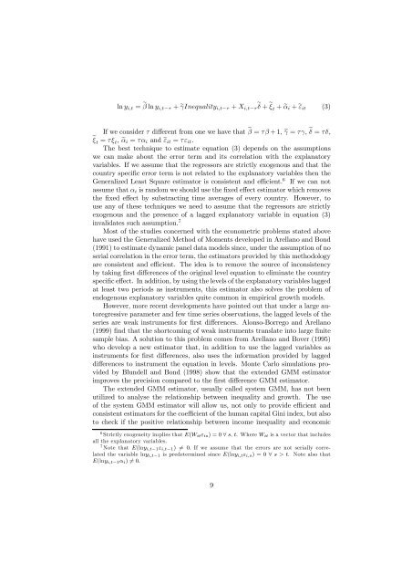
ln y i,t = β ln y i,t−τ + γInequality i,t−τ + X i,t−τ δ + ξt + α i + ε it (3) If we consider τ different from one we have that β = τβ+1, γ = τγ, δ = τδ, ξt = τξ t , α i = τα i and ε it = τε it . The best technique to estimate equation (3) depends on the assumptions we can make about the error term and its correlation with the explanatory variables. If we assume that the regressors are strictly exogenous and that the country specific error term is not related to the explanatory variables then the Generalized Least Square estimator is consistent and efficient. 6 If we can not assume that α i is random we should use the fixed effect estimator which removes the fixed effect by substracting time averages of every country. However, to useanyofthesetechniquesweneedtoassumethattheregressorsarestrictly exogenous and the presence of a lagged explanatory variable in equation (3) invalidates such assumption. 7 Most of the studies concerned with the econometric problems stated above have used the Generalized Method of Moments developed in Arellano and Bond (1991) to estimate dynamic panel data models since, under the assumption of no serial correlation in the error term, the estimators provided by this methodology are consistent and efficient. The idea is to remove the source of inconsistency by taking first differences of the original level equation to eliminate the country specificeffect. In addition, by using the levels of the explanatory variables lagged at least two periods as instruments, this estimator also solves the problem of endogenous explanatory variables quite common in empirical growth models. However, more recent developments have pointed out that under a large autoregressive parameter and few time series observations, the lagged levels of the series are weak instruments for first differences. Alonso-Borrego and Arellano (1999) find that the shortcoming of weak instruments translate into large finite sample bias. A solution to this problem comes from Arellano and Bover (1995) who develop a new estimator that, in addition to use the lagged variables as instruments for first differences, also uses the information provided by lagged differences to instrument the equation in levels. Monte Carlo simulations provided by Blundell and Bond (1998) show that the extended GMM estimator improves the precision compared to the first difference GMM estimator. The extended GMM estimator, usually called system GMM, has not been utilized to analyse the relationship between inequality and growth. The use of the system GMM estimator will allow us, not only to provide efficient and consistent estimators for the coefficient of the human capital Gini index, but also to check if the positive relationship between income inequality and economic 6 Strictly exogeneity implies that E(W it ε is )=0∀ s, t. WhereW it is a vector that includes all the explanatory variables. 7 Note that E(lny i,t−1 ε i,t−1 ) = 0. If we assume that the errors are not serially correlated the variable lny i,t−1 is predetermined since E(lny i,t ε i,s )=0∀ s>t. Note also that E(lny i,t−1 α i ) = 0. 9
Page 1 and 2: A REASSESSMENT OF THE RELATIONSHIP
Page 3 and 4: 1 Introduction In the early 1990s s
Page 5 and 6: capita growth and the investment ra
Page 7: income inequality variables are sti
Page 11 and 12: data set. 9 The explanatory variabl
Page 13 and 14: Table 1- Income Gini coefficients f
Page 15 and 16: Table 2- Cross-section and pool reg
Page 17 and 18: Table 3- Random and Fixed effects R
Page 19 and 20: Sub-Saharan African countries are s
Page 21 and 22: education to real GDP (G/GDP i,t−
Page 23 and 24: ence equation, we also estimate a l
Page 25 and 26: Average Fertility Rate 1960-1 9 8 7
Page 27 and 28: a new generalized method of moments
Page 29 and 30: [6] Atkinson, A. B. and A. Brandoli
Page 31 and 32: 6 Appendix I- Computation of the hu
Page 33: Table A-2- Countries included in th

Amparo CastellÃƒÂ³-Climent, Universidad Carlos III de Madrid ... - Ivie

Create successful ePaper yourself

Delete template?

Save as template?