SPA 3e_ Teachers Edition _ Ch 6

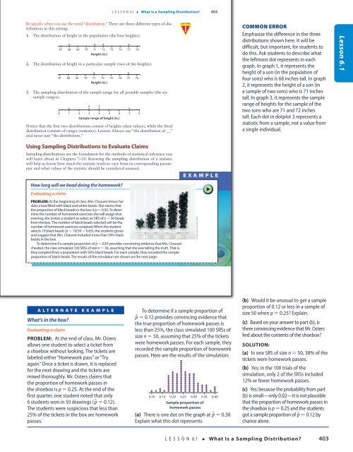
L E S S O N 6.1 • What Is a Sampling Distribution? 403
Be specific when you use the word “distribution.” There are three different types of distributions
in this setting:
1. The distribution of height in the population (the four heights):
d d d d
67 68 69 70 71 72 73 74 75 76
Height (in.)
2. The distribution of height in a particular sample (two of the heights):
d
67 68 69 70 71 72 73 74 75 76
Height (in.)
3. The sampling distribution of the sample range for all possible samples (the six
sample ranges):
d d
d d d d
0 1 2 3 4 5 6 7 8
Sample range of height (in.)
Notice that the first two distributions consist of heights (data values), while the third
distribution consists of ranges (statistics). Lesson: Always use “the distribution of __”
and never just “the distribution.”
d
cAutIOn
!
Common Error
Emphasize the difference in the three
distributions shown here. It will be
difficult, but important, for students to
do this. Ask students to describe what
the leftmost dot represents in each
graph. In graph 1, it represents the
height of a son (in the population of
four sons) who is 68 inches tall. In graph
2, it represents the height of a son (in
a sample of two sons) who is 71 inches
tall. In graph 3, it represents the sample
range of heights for the sample of the
two sons who are 71 and 72 inches
tall. Each dot in dotplot 3 represents a
statistic from a sample, not a value from
a single individual.
Lesson 6.1
Using Sampling Distributions to Evaluate Claims
Sampling distributions are the foundation for the methods of statistical inference you
will learn about in Chapters 7–10. Knowing the sampling distribution of a statistic
will help us know how much the statistic tends to vary from its corresponding parameter
and what values of the statistic should be considered unusual.
How long will we bead doing the homework?
Evaluating a claim
PROBLEM: At the beginning of class, Mrs. Chauvet shows her
class a box filled with black and white beads. She claims that
the proportion of black beads in the box is p 5 0.50. To determine
the number of homework exercises she will assign that
evening, she invites a student to select an SRS of n 5 30 beads
from the box. The number of black beads selected will be the
number of homework exercises assigned. When the student
selects 19 black beads (p^ 5 19/30 5 0.63), the students groan
and suggest that Mrs. Chauvet included more than 50% black
beads in the box.
To determine if a sample proportion of p^ 5 0.63 provides convincing evidence that Mrs. Chauvet
cheated, the class simulated 100 SRSs of size n 5 30, assuming that she was telling the truth. That is,
they sampled from a population with 50% black beads. For each sample, they recorded the sample
proportion of black beads. The results of the simulation are shown on the next page.
e XAMPLe
© Monalyn Gracia/Corbis
18/08/16 4:58 PMStarnes_3e_CH06_398-449_Final.indd 403
Alternate Example
What’s in the box?
Evaluating a claim
PROBLEM: At the end of class, Mr. Osters
allows one student to select a ticket from
a shoebox without looking. The tickets are
labeled either “Homework pass” or “Try
again.” Once a ticket is drawn, it is replaced
for the next drawing and the tickets are
mixed thoroughly. Mr. Osters claims that
the proportion of homework passes in
the shoebox is p 5 0.25. At the end of the
first quarter, one student noted that only
6 students won in 50 drawings ( p^ 5 0.12).
The students were suspicious that less than
25% of the tickets in the box are homework
passes.
18/08/16 4:58 PM
To determine if a sample proportion of
p^ 5 0.12 provides convincing evidence that
the true proportion of homework passes is
less than 25%, the class simulated 100 SRSs of
size n 5 50, assuming that 25% of the tickets
were homework passes. For each sample, they
recorded the sample proportion of homework
passes. Here are the results of the simulation:
d d dddddd d
d d d d d d
d d d d d d
d
d d d d d d d
d d d d d d d
d d d d d d d
d d d d d d d d
d d d d d d d d d d
d d d d d d d d d d d
d d d d d d d d d d d
d
d d d d d d d d d d d d
d d d d
0.10 0.15 0.20 0.25 0.30 0.35 0.40
Sample proportion of
homework passes
(a) There is one dot on the graph at p^ 5 0.38
Explain what this dot represents.
(b) Would it be unusual to get a sample
proportion of 0.12 or less in a sample of
size 50 when p 5 0.25? Explain.
(c) Based on your answer to part (b), is
there convincing evidence that Mr. Osters
lied about the contents of the shoebox?
SOLUTION:
(a) In one SRS of size n 5 50, 38% of the
tickets were homework passes.
(b) Yes; in the 100 trials of the
simulation, only 2 of the SRSs included
12% or fewer homework passes.
(c) Yes; because the probability from part
(b) is small—only 0.02—it is not plausible
that the proportion of homework passes in
the shoebox is p 5 0.25 and the students
got a sample proportion of p^ 5 0.12 by
chance alone.
L E S S O N 6.1 • What Is a Sampling Distribution? 403
Starnes_3e_ATE_CH06_398-449_v3.indd 403
11/01/17 3:53 PM