SPA 3e_ Teachers Edition _ Ch 6

18/08/16 5:03 PMStarnes_3e_CH06_398-449_Final.indd 439
Lesson 6.6
The central Limit Theorem
L e A r n i n g T A r g e T S
d Determine if the sampling distribution of x is approximately normal when
sampling from a non-normal population.
d If appropriate, use a normal distribution to calculate probabilities involving x.
In Lesson 6.5, you learned about the sampling distribution of the sample mean x
when sampling from a normally distributed population. The following activity will
help you explore what happens when you sample from non-normal populations.
AcT iviT y
Sampling from a non-normal population
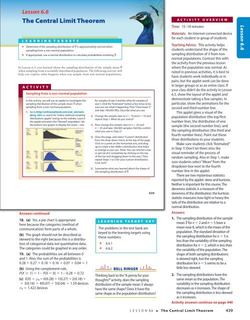
In this activity, we will use an applet to investigate the
sampling distribution of the sample mean x when
sampling from a non-normal population.
1. go to http://onlinestatbook.com/stat_sim/sampling_dist/
or search for “online statbook sampling
distributions applet” and go to the website. Launch
the applet and select the “Skewed” population. Set
the bottom two graphs to display the mean—one
Answers continued
18. (a) Yes, a pie chart is appropriate
here because the categories (method of
communication) form parts of a whole.
(b) The graph should not be described as
skewed to the right because this is a distribution
of categorical data not quantitative data.
The categories could be graphed in any order.
19. (a) The probabilities are all between 0
and 1. Also, the sum of the probabilities is
0.28 1 0.27 1 0.18 1 0.16 1 0.07 1 0.04 5 1
(b) Using the complement rule,
P(X ≥ 1) = 1− P(X = 0) = 1− 0.28 = 0.72
(c) E(X) = m X = 0(0.28) + 1(0.27) + 2(0.18) +
+ 3(0.16) + 4(0.07) + 5(0.04) = 1.59 devices
s X = 1.422 devices
for samples of size 2 and the other for samples of
size 5. Click the “Animated” button a few times to be
sure you see what’s happening. Then “Clear lower 3”
and take 100,000 SRSs. Describe what you see.
2. Change the sample sizes to n 5 10 and n 516 and
repeat Step 1. What do you notice?
3. Now change the sample sizes to n 5 20 and
n 5 25 and take 100,000 samples. Did this confirm
what you saw in Step 2?
4. Clear the page, and select “Custom” distribution
from the drop-down menu at the top of the page.
Click on a point on the horizontal axis, and drag
up to create a bar. Make a distribution that looks
as strange as you can. (Note: You can shorten a bar
or get rid of it completely by clicking on the top
of the bar and dragging down to the axis.) Then
repeat Steps 1 to 3 for your custom distribution.
Cool, huh?
5. Summarize what you learned about the shape of
the sampling distribution of x.
439
Learning Target Key
The problems in the test bank are
keyed to the learning targets using
these numbers:
d 6.6.1
d 6.6.2
18/08/16 5:03 PM
BELL RINGER
Thinking back to the “A penny for your
thoughts?” activity, does the sampling
distribution of the sample mean x always
have the same shape? Does it have the
same shape as the population distribution?
Activity Overview
Time: 15–18 minutes
Materials: An Internet-connected device
for each student or group of students
Teaching Advice: This activity helps
students understand the shape of the
sampling distribution of x from nonnormal
populations. Contrast this with
the activity from the previous lesson
where the population was normal. As
noted in previous activities, it is best to
have students work individually or in
pairs, but the applet work can be done
in larger groups or as an entire class. If
your class didn’t do the activity in Lesson
6.5, show the layout of the applet and
demonstrate taking a few samples. In
particular, show the animations for the
second and third number line.
This applet gives a visual of the
population distribution (the top/first
number line), the distribution of one
sample (the second number line), and
the sampling distribution (the third and
fourth number lines). Point out these
three distributions to your students.
Make sure students click “Animated”
in Step 1! Don’t let them miss the
visual reminder of the process of
random sampling. Also in Step 1, make
sure students select “Mean” from the
dropdown box next to the fourth
number line in the applet.
There are two mysterious statistics
reported by the applet: skew and kurtosis.
Neither is important for this course. The
skewness statistic is a measure of the
skewness of the distribution; the kurtosis
statistic measures how light or heavy the
tails of the distribution are relative to a
normal distribution.
Answers:
1. The sampling distribution of the sample
mean x for n 5 2 and n 5 5 have a
mean near 8, which is the mean of the
population. The standard deviation of
the sampling distribution for n 5 5 is
less than the variability of the sampling
distribution for n 5 2, which is less than
the variability of the population. The
shape of both sampling distributions
is skewed right, but the sampling
distribution for n 5 5 seems to be a
little less skewed.
2. The sampling distributions have the
same mean as the population. The
variability in the sampling distribution
decreases as n increases. The shape of
the sampling distribution is less skewed
as n increases.
Activity answers continue on page 440
Lesson 6.6
L E S S O N 6.6 • The Central Limit Theorem 439
Starnes_3e_ATE_CH06_398-449_v3.indd 439
11/01/17 3:57 PM