SPA 3e_ Teachers Edition _ Ch 6

You also want an ePaper? Increase the reach of your titles
YUMPU automatically turns print PDFs into web optimized ePapers that Google loves.
446<br />
C H A P T E R 6 • Sampling Distributions<br />
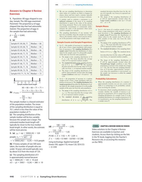
Answers to <strong>Ch</strong>apter 6 Review<br />
Exercises<br />
1. Population: All eggs shipped in one<br />
day. Sample: The 200 eggs examined.<br />
Parameter: The proportion p of eggs<br />
shipped that day that had salmonella.<br />
Statistic: The proportion of eggs in<br />
the sample that had salmonella,<br />
p^ = 9<br />
200 = 0.045.<br />
2. (a)<br />
Sample #1: 64, 66, 71 Median 5 66<br />
Sample #2: 64, 66, 73 Median 5 66<br />
Sample #3: 64, 66, 76 Median 5 66<br />
Sample #4: 64, 71, 73 Median 5 71<br />
Sample #5: 64, 71, 76 Median 5 71<br />
Sample #6: 64, 73, 76 Median 5 73<br />
Sample #7: 66, 71, 73 Median 5 71<br />
Sample #8: 66, 71, 76 Median 5 71<br />
Sample #9: 66, 73, 76 Median 5 73<br />
Sample #10: 71, 73, 76 Median 5 73<br />
d<br />
d<br />
d<br />
d<br />
d<br />
d<br />
66 67 68 69 70 71 72 73<br />
Sample median book length<br />
66 + 66 + 66 + 71 + 71 +<br />
71 + 71 + 73 + 73 + 73<br />
(b) m median =<br />
10<br />
= 701<br />
10 = 70.1<br />
The sample median is a biased estimator<br />
of the population median. The mean<br />
of the sampling distribution is equal to<br />
70.1, which is less than the value of the<br />
population median of 71.<br />
(c) The sampling distribution of the<br />
sample median will be less variable<br />
because the sample size is larger. The<br />
estimated median book length will<br />
typically be closer to the true median<br />
book length. In other words, the estimate<br />
will be more precise.<br />
3. (a) m X = np = 500(0.24) = 120<br />
people; s X = "np(1 − p)<br />
= "500(0.24)(1 − 0.24) = 9.55 people<br />
(b) If many samples of size 500 were<br />
taken, the number of people who are<br />
under 18 years old would typically vary<br />
by about 9.55 from the mean of 120.<br />
(c) The sampling distribution of X<br />
is approximately normal because<br />
np = 500(0.24) = 120 ≥ 10 and<br />
n(1 − p) = 500(1 − 0.24) = 380 ≥ 10<br />
j<br />
j<br />
j<br />
We can use sampling distributions to determine<br />
what values of a statistic are likely to happen by<br />
chance alone and how much a statistic typically<br />
varies from the parameter it is trying to estimate.<br />
A statistic used to estimate a parameter is an<br />
unbiased estimator if the mean of its sampling<br />
distribution is equal to the value of the parameter<br />
being estimated. That is, the statistic doesn’t<br />
consistently overestimate or consistently underestimate<br />
the value of the parameter when many<br />
random samples are selected.<br />
The sampling distribution of any statistic will<br />
have less variability when the sample size is larger.<br />
That is, the statistic will be a more precise estimator<br />
of the parameter with larger sample sizes.<br />
Sample Counts and Sample Proportions<br />
j<br />
j<br />
Let X 5 the number of successes in a random sample<br />
of size n from a large population with proportion<br />
of successes p. The sampling distribution of a<br />
sample count X describes the distribution of values<br />
taken by the sample count X in all possible samples<br />
of the same size from the same population.<br />
j The mean of the sampling distribution of X<br />
is m X = np. The mean describes the average<br />
value of X in repeated random samples.<br />
j The standard deviation of the sampling distribution<br />
of X is s X = !np(1 − p). The standard<br />
deviation describes how far the values of X typically<br />
vary from m X in repeated random samples.<br />
j The shape of the sampling distribution of X<br />
will be approximately normal when the Large<br />
Counts condition is met: np ≥ 10 and n(1 2 p)<br />
≥10.<br />
Let p^ 5 the proportion of successes in a random<br />
sample of size n from a large population with proportion<br />
of successes p. The sampling distribution of a<br />
sample proportion p^ describes the distribution of values<br />
taken by the sample proportion p^ in all possible<br />
samples of the same size from the same population.<br />
j The mean of the sampling distribution of p^ is<br />
m p^ = p. The mean describes the average value<br />
of p^ in repeated random samples.<br />
j The standard deviation of the sampling<br />
p(1 − p)<br />
distribution of p^ is s p^ 5 . The<br />
Å n<br />
Starnes_<strong>3e</strong>_CH06_398-449_Final.indd 446<br />
100 − 120<br />
(d) z = = −2.09;<br />
9.55<br />
110 − 120<br />
z = = −1.05<br />
9.55<br />
P(100 ≤ X ≤ 110) ≈ P(−2.09 ≤<br />
Z ≤ − 1.05) = 0.1469 − 0.0183 = 0.1286<br />
Using technology: Applet/normalcdf<br />
(lower:100, upper:110, mean:120, SD:9.55)<br />
5 0.1294<br />
j<br />
standard deviation describes how far the values<br />
of p^ typically vary from p in repeated random<br />
samples.<br />
The shape of the sampling distribution of<br />
p^ will be approximately normal when the<br />
Large Counts condition is met: np ≥ 10 and<br />
n(1 2 p) ≥ 10.<br />
Sample Means<br />
j<br />
j<br />
Let x 5 the mean of a random sample of size n<br />
from a large population with mean m and standard<br />
deviation s. The sampling distribution of<br />
a sample mean x describes the distribution of<br />
values taken by the sample mean x in all possible<br />
samples of the same size from the same<br />
population.<br />
j The mean of the sampling distribution of x is<br />
m x = m. The mean describes the average value<br />
of x in repeated random samples.<br />
j The standard deviation of the sampling distribution<br />
of x is s− x = s . The standard deviation<br />
describes how far the values of x typically<br />
"n<br />
vary from m in repeated random samples.<br />
The shape of the sampling distribution of<br />
x will be approximately normal when the<br />
Normal/Large Sample condition is met: The<br />
population is normal or the sample size is large<br />
(n ≥ 30). The fact that the sampling distribution<br />
of x becomes approximately normal—<br />
even when the population is non-normal—as<br />
the sample size increases is called the central<br />
limit theorem.<br />
Probability Calculations<br />
j<br />
j<br />
When the sampling distribution of a statistic is<br />
approximately normal, you can use z-scores and<br />
Table A or technology to do probability calculations<br />
involving the statistic.<br />
To determine which sampling distribution to use,<br />
consider whether the variable of interest is categorical<br />
or quantitative. If it is categorical, use the<br />
sampling distribution of a sample count X or the<br />
sampling distribution of a sample proportion p^ . If<br />
it is quantitative, use the sampling distribution of<br />
a sample mean x.<br />
TRM chapter 6 Review Exercise Videos<br />
Video solutions to the <strong>Ch</strong>apter 6 Review<br />
Exercises are available to teachers and<br />
students. Access them by clicking on the link<br />
in the TE-book, logging into the Teacher’s<br />
Resource site, or accessing this resource<br />
on the TRFD.<br />
18/08/16 5:04 PMStarnes_<strong>3e</strong>_CH0<br />
446<br />
C H A P T E R 6 • Sampling Distributions<br />
Starnes_<strong>3e</strong>_ATE_CH06_398-449_v3.indd 446<br />
11/01/17 3:58 PM