SPA 3e_ Teachers Edition _ Ch 6

L E S S O N 6.2 • Sampling Distributions: Center and Variability 411
Statistic 1
Statistic 2
0 20 40 60 80 100 120 140 160 180 200
Estimated variance
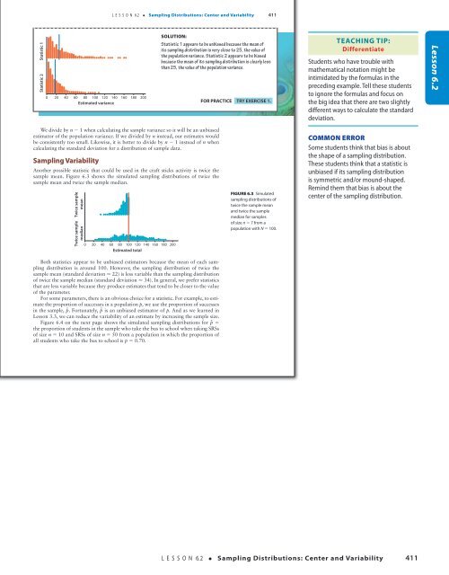
SOLUTION:
Statistic 1 appears to be unbiased because the mean of
its sampling distribution is very close to 25, the value of
the population variance. Statistic 2 appears to be biased
because the mean of its sampling distribution is clearly less
than 25, the value of the population variance.
FOR PRACTICE TRY EXERCISE 1.
Teaching Tip:
Differentiate
Students who have trouble with
mathematical notation might be
intimidated by the formulas in the
preceding example. Tell these students
to ignore the formulas and focus on
the big idea that there are two slightly
different ways to calculate the standard
deviation.
Lesson 6.2
We divide by n 2 1 when calculating the sample variance so it will be an unbiased
estimator of the population variance. If we divided by n instead, our estimates would
be consistently too small. Likewise, it is better to divide by n 2 1 instead of n when
calculating the standard deviation for a distribution of sample data.
Sampling Variability
Another possible statistic that could be used in the craft sticks activity is twice the
sample mean. Figure 6.3 shows the simulated sampling distributions of twice the
sample mean and twice the sample median.
Twice sample
mean
Twice sample
median
d
dd
d ddd dddd
d
d
d
d
d
d d dd d d d d dd
dd ddddddddd
dd d d dddddd
ddd d d d dddd
0 20 40 60 80 100 120 140 160 180 200
Estimated total
Both statistics appear to be unbiased estimators because the mean of each sampling
distribution is around 100. However, the sampling distribution of twice the
sample mean (standard deviation ≈ 22) is less variable than the sampling distribution
of twice the sample median (standard deviation ≈ 34). In general, we prefer statistics
that are less variable because they produce estimates that tend to be closer to the value
of the parameter.
For some parameters, there is an obvious choice for a statistic. For example, to estimate
the proportion of successes in a population p, we use the proportion of successes
in the sample, p^ . Fortunately, p^ is an unbiased estimator of p. And as we learned in
Lesson 3.3, we can reduce the variability of an estimate by increasing the sample size.
Figure 6.4 on the next page shows the simulated sampling distributions for p^ 5
the proportion of students in the sample who take the bus to school when taking SRSs
of size n 5 10 and SRSs of size n 5 50 from a population in which the proportion of
all students who take the bus to school is p 5 0.70.
FigUre 6.3 Simulated
sampling distributions of
twice the sample mean
and twice the sample
median for samples
of size n 5 7 from a
population with N 5 100.
Common Error
Some students think that bias is about
the shape of a sampling distribution.
These students think that a statistic is
unbiased if its sampling distribution
is symmetric and/or mound-shaped.
Remind them that bias is about the
center of the sampling distribution.
18/08/16 4:59 PMStarnes_3e_CH06_398-449_Final.indd 411
18/08/16 5:00 PM
L E S S O N 6.2 • Sampling Distributions: Center and Variability 411
Starnes_3e_ATE_CH06_398-449_v3.indd 411
11/01/17 3:54 PM