differential equation

Differential equations
49
Numerical methods for first order
differential equations
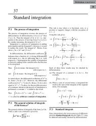
49.1 Introduction
Not all first order differential equations may be
solved by separating the variables (as in Chapter 46)
or by the integrating factor method (as in Chapter
48). A number of other analytical methods of
solving differential equations exist. However the
differential equations that can be solved by such
analytical methods is fairly restricted.
Where a differential equation and known boundary
conditions are given, an approximate solution
may be obtained by applying a numerical method.
There are a number of such numerical methods available
and the simplest of these is called Euler’s
method.
49.2 Euler’s method
From Chapter 8, Maclaurin’s series may be stated as:
f (x) = f (0) + xf ′ (0) + x2
2! f ′′ (0) +···
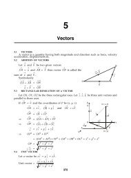
Hence at some point f (h) in Fig. 51.1:
f (h) = f (0) + hf ′ (0) + h2
2! f ′′ (0) +···
P
y
0
f(0)
h
Q
f(h)
x
y = f(x)
Figure 49.1
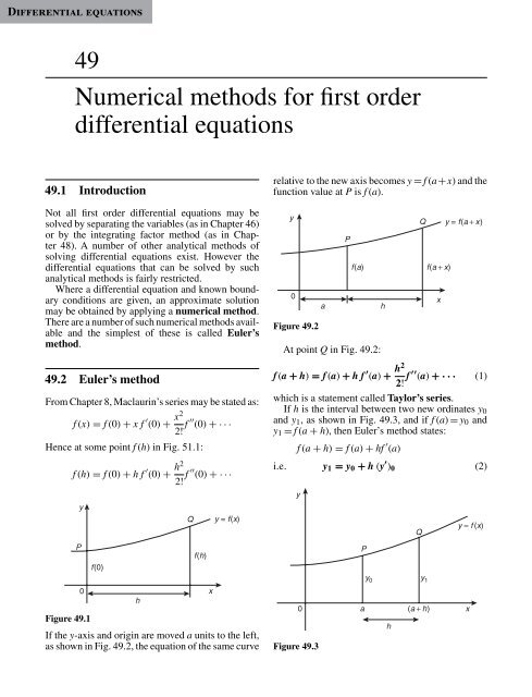
If the y-axis and origin are moved a units to the left,
as shown in Fig. 49.2, the equation of the same curve
relative to the new axis becomes y = f (a+x) and the
function value at P is f (a).
y
0
Figure 49.2
a
P
At point Q in Fig. 49.2:
f(a) f(a + x)
h
Q y = f(a + x)
f (a + h) = f (a) + hf ′ (a) + h2
2! f ′′ (a) +··· (1)
which is a statement called Taylor’s series.
If h is the interval between two new ordinates y 0
and y 1 , as shown in Fig. 49.3, and if f (a) = y 0 and
y 1 = f (a + h), then Euler’s method states:
f (a + h) = f (a) + hf ′ (a)
i.e. y 1 = y 0 + h (y ′ ) 0 (2)
y
0
Figure 49.3
Q
y = f (x)
P
a (a + h) x
h
x