differential equation

472 DIFFERENTIAL EQUATIONS
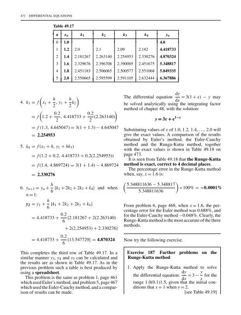
Table 49.17
n x n k 1 k 2 k 3 k 4 y n
0 1.0 4.0
1 1.2 2.0 2.1 2.09 2.182 4.418733
2 1.4 2.181267 2.263140 2.254953 2.330276 4.870324
3 1.6 2.329676 2.396708 2.390005 2.451675 5.348817
4 1.8 2.451183 2.506065 2.500577 2.551068 5.849335
5 2.0 2.550665 2.595599 2.591105 2.632444 6.367886
(
4. k 3 = f x 1 + h 2 , y 1 + h )
2 k 2
(
= f 1.2 + 0.2
)
0.2
,4.418733 +
2 2 (2.263140)
= f (1.3, 4.645047) = 3(1 + 1.3) − 4.645047
= 2.254953
5. k 4 = f (x 1 + h, y 1 + hk 3 )
= f (1.2 + 0.2, 4.418733 + 0.2(2.254953))
= f (1.4, 4.869724) = 3(1 + 1.4) − 4.869724
= 2.330276
6. y n+1 = y n + h 6 {k 1 + 2k 2 + 2k 3 + k 4 } and when
n = 1:
y 2 = y 1 + h 6 {k 1 + 2k 2 + 2k 3 + k 4 }
= 4.418733 + 0.2 {2.181267 + 2(2.263140)
6
+ 2(2.254953) + 2.330276}
= 4.418733 + 0.2 {13.547729} =4.870324
6
This completes the third row of Table 49.17. In a
similar manner y 3 , y 4 and y 5 can be calculated and
the results are as shown in Table 49.17. As in the
previous problem such a table is best produced by
using a spreadsheet.
This problem is the same as problem 1, page 461
which used Euler’s method, and problem 5, page 467
which used the Euler-Cauchy method, and a comparison
of results can be made.
The differential equation dy = 3(1 + x) − y may
dx
be solved analytically using the integrating factor
method of chapter 48, with the solution:
y = 3x + e 1−x
Substituting values of x of 1.0, 1.2, 1.4, ..., 2.0 will
give the exact values. A comparison of the results
obtained by Euler’s method, the Euler-Cauchy
method and the Runga-Kutta method, together
with the exact values is shown in Table 49.18 on
page 473.
It is seen from Table 49.18 that the Runge-Kutta
method is exact, correct to 4 decimal places.
The percentage error in the Runge-Kutta method
when, say, x = 1.6 is:
( )
5.348811636 − 5.348817
×100% = −0.0001%
5.348811636
From problem 6, page 468, when x = 1.6, the percentage
error for the Euler method was 0.688%, and
for the Euler-Cauchy method −0.048%. Clearly, the
Runge-Kutta method is the most accurate of the three
methods.
Now try the following exercise.
Exercise 187 Further problems on the
Runge-Kutta method
1. Apply the Runge-Kutta method to solve
the differential equation: dy
dx = 3 − y for the
x
range 1.0(0.1)1.5, given that the initial conditions
that x = 1 when y = 2.
[see Table 49.19]