differential equation

Differential equations 

46 

Solution of first order differential 

equations by separation of variables 

I 

46.1 Family of curves 

Integrating both sides of the derivative dy 

dx = 3 with 

respect to x gives y = ∫ 3dx, i.e., y = 3x + c, where 

c is an arbitrary constant. 

y = 3x + c represents a family of curves, each of 

the curves in the family depending on the value of 

c. Examples include y = 3x + 8, y = 3x + 3, y = 3x 

and y = 3x − 10 and these are shown in Fig. 46.1. 

Integrating both sides of dy = 4x with respect to x 

dx 

gives: 

∫ ∫ dy 

dx dx = 4x dx, i.e., y = 2x 2 + c 

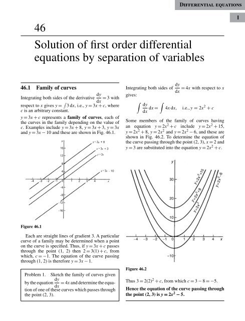
Some members of the family of curves having 

an equation y = 2x 2 + c include y = 2x 2 + 15, 

y = 2x 2 + 8, y = 2x 2 and y = 2x 2 − 6, and these are 

shown in Fig. 46.2. To determine the equation of 

the curve passing through the point (2, 3), x = 2 and 

y = 3 are substituted into the equation y = 2x 2 + c. 

Figure 46.1 

Each are straight lines of gradient 3. A particular 

curve of a family may be determined when a point 

on the curve is specified. Thus, if y = 3x + c passes 

through the point (1, 2) then 2 = 3(1) + c, from 

which, c =−1. The equation of the curve passing 

through (1, 2) is therefore y = 3x − 1. 

Problem 1. Sketch the family of curves given 

by the equation dy = 4x and determine the equation 

of one of these curves which passes through 

dx 

the point (2, 3). 

Figure 46.2 

Thus 3 = 2(2) 2 + c, from which c = 3 − 8 =−5. 

Hence the equation of the curve passing through 

the point (2, 3) is y = 2x 2 − 5.

444 DIFFERENTIAL EQUATIONS 

Now try the following exercise. 

Exercise 177 Further problems on families 

of curves 

1. Sketch a family of curves represented by each 

of the following differential equations: 

(a) dy dy dy 

= 6 (b) = 3x (c) 

dx dx dx = x + 2 

2. Sketch the family of curves given by the equation 

dy = 2x + 3 and determine the equation 

dx 

of one of these curves which passes through 

the point (1, 3). [y = x 2 + 3x − 1] 

46.2 Differential equations 

A differential equation is one that contains differential 

coefficients. 

Examples include 

(i) dy 

dx = 7x and (ii) d2 y 

dx 2 + 5 dy 

dx + 2y = 0 

Differential equations are classified according to the 

highest derivative which occurs in them. Thus example 

(i) above is a first order differential equation, 

and example (ii) is a second order differential 

equation. 

The degree of a differential equation is that of the 

highest power of the highest differential which the 

equation contains after simplification. 

( d 2 ) 3 ( ) 

x dx 5 

Thus 

dt 2 + 2 = 7 is a second order 

dt 

differential equation of degree three. 

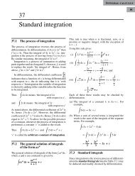
Starting with a differential equation it is possible, 

by integration and by being given sufficient data to 

determine unknown constants, to obtain the original 

function. This process is called ‘solving the 

differential equation’. A solution to a differential 

equation which contains one or more arbitrary constants 

of integration is called the general solution 

of the differential equation. 

When additional information is given so that constants 

may be calculated the particular solution of 

the differential equation is obtained. The additional 

information is called boundary conditions. Itwas 

shown in Section 46.1 that y = 3x + c is the general 

solution of the differential equation dy 

dx = 3. 

Given the boundary conditions x = 1 and y = 2, 

produces the particular solution of y = 3x − 1. 

Equations which can be written in the form 

dy dy 

dy 

= f (x), = f (y) and = f (x) · f (y) 

dx dx dx 

can all be solved by integration. In each case it is 

possible to separate the y’s to one side of the equation 

and the x’s to the other. Solving such equations 

is therefore known as solution by separation of 

variables. 

46.3 The solution of equations of the 

form dy 

dx = f (x) 

A differential equation of the form dy 

dx 

solved by direct integration, 

∫ 

i.e. y = 

f (x) dx 

= f (x) is 

Problem 2. Determine the general solution of 

x dy 

dx = 2 − 4x3 

Rearranging x dy 

dx = 2 − 4x3 gives: 

dy 

dx = 2 − 4x3 = 2 x x − 4x3 = 2 x x − 4x2 

Integrating both sides gives: 

∫ ( ) 2 

y = 

x − 4x2 dx 

i.e. y = 2lnx − 4 3 x3 + c, 

which is the general solution. 

Problem 3. Find the particular solution of the 

differential equation 5 dy + 2x = 3, given the 

dx 

boundary conditions y = 1 2 when x = 2. 

5

SOLUTION OF FIRST ORDER DIFFERENTIAL EQUATIONS BY SEPARATION OF VARIABLES 445 

Since 5 dy 

dy 

+ 2x = 3 then 

dx 

Hence y = 

i.e. 

∫ ( 3 

5 − 2x 

5 

y = 3x 

5 − x2 

5 + c, 

dx = 3 − 2x 

5 

) 

dx 


= 3 5 − 2x 

5 

Substituting the boundary conditions y = 1 2 5 

and 

x = 2 to evaluate c gives: 

1 2 5 = 6 5 − 4 5 

+ c, from which, c = 1 

Hence the particular solution is y = 3x 

5 − x2 

5 + 1. 

Problem ( 4. Solve the equation 

2t t − dθ ) 

= 5, given θ = 2 when t = 1. 

dt 

Rearranging gives: 

t − dθ 

dt = 5 and 

2t 

Integrating gives: 

∫ ( 

θ = t − 5 ) 

dt 

2t 

dθ 

dt = t − 5 2t 

i.e. θ = t2 2 − 5 ln t + c, 

2 


When θ = 2, t = 1, thus 2 = 

2 1 − 2 5 ln 1 + c from 

which, c = 

2 3 . 

Hence the particular solution is: 

θ = t2 2 − 5 2 ln t + 3 2 

i.e. θ = 1 2 (t2 − 5lnt + 3) 

Problem 5. The bending moment M of the 

beam is given by dM =−w(l − x), where w and 

dx 

x are constants. Determine M in terms of x given: 

M = 

2 1 wl2 when x = 0. 

dM 

dx 

=−w(l − x) =−wl + wx 

Integrating 

with respect to x gives: 

M =−wlx + wx2 

2 + c 


When M = 

2 1 wl2 , x = 0. 

Thus 1 2 wl2 =−wl(0) + w(0)2 + c 

2 

from which, c = 1 2 wl2 . 


M =−wlx + w(x)2 + 1 2 2 wl2 

i.e. M = 1 2 w(l2 − 2lx + x 2 ) 

or M = 1 w(l − x)2 

2 


Exercise 178 Further problems on equations 

of the form dy 

dx = f (x). 

In Problems 1 to 5, solve the differential 

equations. 

[ 

] 

dy 

1. 

dx = cos 4x − 2x sin 4x 

y = − x 2 + c 

4 

2. 2x dy 

[ 

dx = 3 − x3 y = 3 ] 

x3 

ln x − 

2 6 + c 

dy 

3. + x = 3, given y = 2 when x = 1. 

dx 

[y = 3x − x2 

2 − 1 ] 

2 

4. 3 dy 

dθ + sin θ = 0, given y = 2 3 when θ = π [ 

3 

y = 1 3 cos θ + 1 ] 

2 

5. 

1 

e x + 2 = x − 3dy ,giveny = 1 when x = 0. 

dx 

[ 

y = 1 (x 2 − 4x + 2 )] 

6 

e x + 4 

6. The gradient of a curve is given by: 

dy 

dx + x2 

2 = 3x 

I


Find the equation of the curve if it passes 

through the point ( 1, 1 ) 

3 . 

[ 

y = 3 ] 

2 x2 − x3 

6 − 1 

7. The acceleration, a, of a body is equal to its 

rate of change of velocity, dv . Find an equation 

for v in terms of t, given that when t = 0, 

dt 

velocity v = u. 

[v = u + at] 

8. An object is thrown vertically upwards with 

an initial velocity, u, of 20 m/s. The motion 

of the object follows the differential equation 

ds 

= u−gt, where s is the height of the object 

dt 

in metres at time t seconds and g = 9.8m/s 2 . 

Determine the height of the object after 3 

seconds if s = 0 when t = 0. [15.9 m] 


form dy 

dx = f ( y) 

A differential equation of the form dy = f (y) is 

dx 

initially rearranged to give dx = dy and then the 

f (y) 

solution is obtained by direct integration, 

i.e. 

∫ 

∫ 

dx = 

dy 

f ( y) 

Problem 6. Find the general solution of 

dy 

dx = 3 + 2y. 

Rearranging dy = 3 + 2y gives: 

dx 

dx = 

dy 

3 + 2y 


∫ 

∫ 

dx = 

dy 

3 + 2y 

Thus, by using the substitution u = (3 + 2y) — see 

Chapter 39, 

x = 

2 1 ln (3 + 2y) + c (1) 

It is possible to give the general solution of a differential 

equation in a different form. For example, if 

c = ln k, where k is a constant, then: 

x = 

2 1 ln(3 + 2y) + ln k, 

i.e. x = ln(3 + 2y) 2 1 + ln k 

or x = ln [k √ (3 + 2y)] (2) 

by the laws of logarithms, from which, 

e x = k √ (3 + 2y) (3) 

Equations (1), (2) and (3) are all acceptable general 

solutions of the differential equation 

dy 

dx = 3 + 2y 

Problem 7. Determine the particular solution 

of (y 2 − 1) dy = 3y given that y = 1 when 

dx 

x = 2 1 6 


( y 2 − 1 

dx = 

3y 

Integrating gives: 

∫ 

dx = 

) ( y 

dy = 

3 − 1 ) 

dy 

3y 

∫ ( y 

3 − 1 3y 

) 

dy 

i.e. x = y2 

6 − 1 ln y + c, 

3 


When y = 1, x = 2 1 6 , thus 2 1 6 = 1 6 − 1 3 

ln 1 + c, from 

which, c = 2. 


x = y2 

6 − 1 3 ln y + 2 

Problem 8. (a) The variation of resistance, 

R ohms, of an aluminium conductor with 

temperature θ ◦ C is given by dR = αR, where 

dθ

α is the temperature coefficient of resistance of 

aluminium. If R = R 0 when θ = 0 ◦ C, solve the 

equation for R. (b) If α = 38 × 10 −4 / ◦ C, determine 

the resistance of an aluminium conductor 

at 50 ◦ C, correct to 3 significant figures, when its 

resistance at 0 ◦ C is 24.0 . 

(a) dR 

dy 

= αR is of the form 

dθ dx = f (y) 

Rearranging gives: dθ = dR 

αR 


∫ ∫ dR 

dθ = 

αR 


1. 

2. 

[ 

dy 

dx = 2 + 3y x = 1 ] 

3 ln (2 + 3y) + c 

dy 

dx = 2 cos2 y [ tan y = 2x + c] 

3. (y 2 + 2) dy 

dx = 5y, giveny = 1 when x = 1 2 

[ y 

2 

2 + 2lny = 5x − 2 ] 

4. The current in an electric circuit is given by 

the equation 

Ri + L di 

dt = 0, 

i.e., θ = 1 ln R + c, 

α 


Substituting the boundary conditions R = R 0 

when θ = 0 gives: 

0 = 1 α ln R 0 + c 

from which c =− 1 α ln R 0 

Hence the particular solution is 

θ = 1 α ln R − 1 α ln R 0 = 1 α (ln R − ln R 0) 

i.e. θ = 1 ( ) ( ) 

R R 

α ln or αθ = ln 

R 0 R 0 

Hence e αθ = R R 0 

from which, R = R 0 e αθ . 

(b) Substituting α = 38 × 10 −4 , R 0 = 24.0 and θ = 

50 into R = R 0 e αθ gives the resistance at 50 ◦ C, 

i.e., R 50 = 24.0e (38×10−4 ×50) = 29.0 ohms. 




dx = f ( y) 

In Problems 1 to 3, solve the differential 


where L and R are constants. Show that 

i = Ie −Rt 

L , given that i = I when t = 0. 

5. The velocity of a chemical reaction is given 

by dx = k(a − x), where x is the amount 

dt 

transferred in time t, k is a constant and a 

is the concentration at time t = 0 when x = 0. 

Solve the equation and determine x in terms 

of t. [x = a(1 − e −kt )] 

6.(a) Charge Q coulombs at time t seconds 

is given by the differential equation 

R dQ 

dt + Q = 0, where C is the capacitance 

in farads and R the resistance in 

C 

ohms. Solve the equation for Q given that 

Q = Q 0 when t = 0. 

(b) A circuit possesses a resistance of 

250 × 10 3 and a capacitance of 

8.5 × 10 −6 F, and after 0.32 seconds the 

charge falls to 8.0 C. Determine the initial 

charge and the charge after 1 second, 

each correct to 3 significant figures. 

[(a) Q = Q 0 e CR −t 

(b) 9.30 C, 5.81 C] 

7. A differential equation relating the difference 

in tension T, pulley contact angle θ and coefficient 

of friction µ is dT = µT. When θ = 0, 

dθ 

T = 150 N, and µ = 0.30 as slipping starts. 

Determine the tension at the point of slipping 

when θ = 2 radians. Determine also the value 

of θ when T is 300 N. [273.3 N, 2.31 rads] 

I


8. The rate of cooling of a body is given by 

dθ 

dt = kθ, where k is a constant. If θ = 60◦ C 

when t = 2 minutes and θ = 50 ◦ C when 

t = 5 minutes, determine the time taken for θ 

to fall to 40 ◦ C, correct to the nearest second. 

[8 m 40 s] 


form dy = f (x) · f ( y) 

dx 

A differential equation of the form dy = f (x) · f (y), 

dx 

where f (x) is a function of x only and f (y) is a function 

of y only, may be rearranged as dy 

f (y) = f (x)dx, 

and then the solution is obtained by direct integration, 

i.e. 

∫ 

Problem 9. 

∫ dy 

f (y) = 

f (x)dx 

Solve the equation 4xy dy 

dx = y2 −1 

Separating the variables gives: 

( ) 4y 

y 2 dy = 1 − 1 x dx 


∫ ( ) ∫ ( ) 

4y 

1 

y 2 dy = dx 

− 1 

x 

Using the substitution u = y 2 − 1, the general 

solution is: 

2ln(y 2 − 1) = ln x + c (1) 

or ln (y 2 − 1) 2 − ln x = c 

{ (y 2 − 1) 2 } 

from which, ln 

= c 

x 

( y 2 − 1) 2 

and 

= e c (2) 

x 

If in equation (1), c = ln A, where A is a different 

constant, 

then 

ln (y 2 − 1) 2 = ln x + ln A 

i.e. ln (y 2 − 1) 2 = ln Ax 

i.e. ( y 2 − 1) 2 = Ax (3) 

Equations (1) to (3) are thus three valid solutions of 

the differential equations 

4xy dy 

dx = y2 − 1 


of dθ 

dt = 2e3t−2θ , given that t = 0 when θ = 0. 

dθ 

dt = 2e3t−2θ = 2(e 3t )(e −2θ ), 

by the laws of indices. 


dθ 

e −2θ = 2e3t dt, 

i.e. e 2θ dθ = 2e 3t dt 


∫ ∫ 

e 2θ dθ = 2e 3t dt 

Thus the general solution is: 

1 

2 e2θ = 2 3 e3t + c 

When t = 0, θ = 0, thus: 

1 

2 e0 = 2 3 e0 + c 

from which, c = 1 2 − 2 3 =−1 6 


1 

2 e2θ = 2 3 e3t − 1 6 

or 3e 2θ = 4e 3t − 1 

Problem 11. Find the curve which satisfies the 

equation xy = (1 + x 2 ) dy and passes through the 

dx 

point (0, 1). 


x dy 

(1 + x 2 dx = 

) y



1 

2 ln (1 + x2 ) = ln y + c 

1 

When x = 0, y = 1 thus 

2 

ln 1 = ln 1 + c, from 

which, c = 0. 

Hence the particular solution is 1 2 ln (1 + x2 ) = ln y 

i.e. ln (1 + x 2 ) 1 2 = ln y, from which, (1 + x 2 ) 1 2 = y. 

Hence the equation of the curve is y = √ (1 + x 2 ). 

Hence the general solution is: 

− 1 R ln (E − Ri) = t L + c 

(by making a substitution u = E − Ri, see 

Chapter 39). 

When t = 0, i = 0, thus − 1 R ln E = c 

Thus the particular solution is: 

Problem 12. The current i in an electric circuit 

containing resistance R and inductance L in 

series with a constant voltage source( E is) 

given 

di 

by the differential equation E − L = Ri. 

dt 

Solve the equation and find i in terms of time 

t given that when t = 0, i = 0. 

In the R − L series circuit shown in Fig. 46.3, the 

supply p.d., E, isgivenby 

Hence 

from which 

E = V R + V L 

V R = iR and V L = L di 

dt 

E = iR + L di 

dt 

E − L di 

dt = Ri 

V R 

R 

L 

V L 

− 1 R ln (E − Ri) = t L − 1 R ln E 

Transposing gives: 

− 1 R ln (E − Ri) + 1 R ln E = t L 

1 

R [ln E − ln (E − Ri)] = t L 

( ) E 

ln = Rt 

E − Ri L 

E 

from which 

E − Ri = e Rt 

L 

Hence 

E − Ri 

E 

Ri = E − Ee −Rt 

Hence current, 

i = E R 

L . 

= e −Rt 

L and E − Ri = Ee −Rt 

L 

( ) 

1 − e −Rt 

L , 

and 

i 

E 

which represents the law of growth of current in an 

inductive circuit as shown in Fig. 46.4. 

I 

Figure 46.3 

Most electrical circuits can be reduced to a differential 

equation. 

Rearranging E − L di di 

= Ri gives 

dt dt = E − Ri 

L 

and separating the variables gives: 

di 

E − Ri = dt 

L 


∫ ∫ 

di dt 

E − Ri = L 

i 

E 

R 

0 

Figure 46.4 

i = E R 

(l −e -Rt/L ) 

Time t


Problem 13. For an adiabatic expansion of 2. (2y − 1) dy 

agas 

dx = (3x2 + 1), given x = 1 when 

y = 2. [y 2 − y = x 3 + x] 

dp 

C v 

p + C dV 

p 

V = 0, 

dy 

3. 

dx = e2x−y ,givenx = 0 when y = 0. 

where C p and C v are constants. Given n = C [ 

p 

, 

e 

C y = 1 

v 

show that pV n 2 e2x + 1 ] 

2 

= constant. 

4. 2y(1 − x) + x(1 + y) dy = 0, given x = 1 

dx 


when y = 1. [ln (x 2 y) = 2x − y − 1] 

dp 

C v 

p =−C dV 

5. Show that the solution of the equation 

p 

V 

y 2 + 1 

x 2 + 1 = y dy 

is of the form 

x dx 


√ (y 2 ) 

+ 1 

∫ ∫ dp dV x 2 = constant. 

+ 1 

C v 

p =−C p 

V 

6. Solve xy = (1 − x 2 ) dy for y, given x = 0 

dx [ 

] 

i.e. C v ln p =−C p ln V + k 

1 

when y = 1. 

y = √ 

(1 − x 2 ) 

Dividing throughout by constant C v gives: 

ln p =− C p 

ln V + k 7. Determine the equation of the curve which 

satisfies the equation xy dy 

C v C v 

dx = x2 − 1, and 

which passes through the point (1, 2). 

Since C p 

= n, then ln p + n ln V = K, 

[y 2 = x 2 − 2lnx + 3] 

C v 

where K = k 8. The p.d., V, between the plates of a capacitor 

C charged by a steady voltage E 

. 

C v through a resistor R is given by the equation 

i.e. ln p + ln V n = K or ln pV n = K, by the laws of CR dV 

logarithms. 

dt + V = E. 

Hence pV n = e K , i.e., pV n (a) Solve the equation for V given that at 

= constant. 

t = 0, V = 0. 

(b) Calculate V, correct to 3 significant figures, 

when E = 25 V, C = 20 ×10 −6 F, 


R = 200 ×10 3 and t = 3.0s. 

⎡ 

( ) ⎤ 



⎣ (a) V = E 1 − e CR 

−t 

⎦ 

= f (x) · f (y) 

dx (b) 13.2V 

In Problems 1 to 4, solve the differential 9. Determine the value of p, given that 


x 3 dy = p − x, and that y = 0 when x = 2 and 

dy 

1. 

dx = 2y cos x [ln y = 2 sin x + c] dx 

when x = 6. [3]


47 

Homogeneous first order differential 

equations 

47.1 Introduction 

Certain first order differential equations are not of the 

‘variable-separable’ type, but can be made separable 

by changing the variable. 

An equation of the form P dy = Q, where P and 

dx 

Q are functions of both x and y of the same degree 

throughout, is said to be homogeneous in y and x. 

For example, f (x, y) = x 2 + 3xy + y 2 is a homogeneous 

function since each of the three terms are of 

degree 2. However, f (x, y) = x2 − y 

2x 2 is not homogeneous 

since the term in y in the numerator is of 

+ y2 degree 1 and the other three terms are of degree 2. 

47.2 Procedure to solve differential 

equations of the form P dy 

dx = Q 

(i) Rearrange P dy 

dy 

= Q into the form 

dx dx = Q P 

(ii) Make the substitution y = vx (where v is a function 

of x), from which, dy dv 

= v(1) + x , by the 

dx dx 

product rule. 

(iii) Substitute for both y and dy in the equation 

dy 

dx = Q . Simplify, by cancelling, and an 

dx 

P 

equation results in which the variables are 

separable. 

(iv) Separate the variables and solve using the 

method shown in Chapter 46. 

(v) Substitute v = y to solve in terms of the original 

x 

variables. 

47.3 Worked problems on 

homogeneous first order 

differential equations 

Problem 1. Solve the differential equation: 

y − x = x dy ,givenx = 1 when y = 2. 

dx 

Using the above procedure: 

(i) Rearranging y − x = x dy 

dx gives: 

dy 

dx = y − x , 

x 

which is homogeneous in x and y. 

(ii) Let y = vx, then dy 

dx = v + x dv 

dx 

(iii) Substituting for y and dy 

dx gives: 

v + x dv 

dx = vx − x x(v − 1) 

= = v − 1 

x x 

(iv) Separating the variables gives: 

x dv 

dx = v − 1 − v =−1, i.e. dv =−1 x dx 


∫ ∫ 

dv = − 1 x dx 

Hence, v =−ln x + c 

(v) Replacing v by y x gives: y =−ln x + c, which 

x 

is the general solution. 

When x = 1, y = 2, thus: 2 =−ln 1 + c from 

1 

which, c = 2 

I


Thus, the particular solution is: y x =−ln x + 2 

or y =−x(ln x − 2) or y = x(2 − ln x) 

Problem 2. Find the particular solution of the 

equation: x dy 

dx = x2 + y 2 

, given the boundary 

y 

conditions that y = 4 when x = 1. 

Using the procedure of section 47.2: 

(i) Rearranging x dy 

dx = x2 + y 2 

gives: 

y 

dy 

dx = x2 + y 2 

which is homogeneous in x and 

xy 

y since each of the three terms on the right hand 

side are of the same degree (i.e. degree 2). 

(ii) Let y = vx then dy 

dx = v + x dv 

dx 


dx 

dy 

dx = x2 + y 2 

gives: 

xy 

v + x dv 

dx = x2 + v 2 x 2 

x(vx) 

= x2 + v 2 x 2 

vx 2 


in the equation 

= 1 + v2 

v 

x dv 

dx = 1 + v2 

− v = 1 + v2 − v 2 

= 1 v 

v v 

Hence, v dv = 1 x dx 


∫ ∫ 1 v2 

v dv = dx i.e. 

x 2 = ln x + c 

(v) Replacing v by y x gives: y 2 

= ln x + c, which 

2x2 is the general solution. 

16 

When x = 1, y = 4, thus: = ln 1 + c from 

2 

which, c = 8 

Hence, the particular solution is: y2 

2x 2 = ln x + 8 

or y 2 = 2x 2 (8 + ln x) 


Exercise 181 Further problems on homogeneous 

first order differential equations 

1. Find the general solution of: x 2 = y 2 dy 

dx 

[− 1 ( x 3 

3 ln − y 3 ) ] 

x 3 = ln x + c 

2. Find the general solution of: 

x − y + x dy 

dx = 0 [y = x(c − ln x)] 

3. Find the particular solution of the differential 

equation: (x 2 + y 2 )dy = xy dx, given that 

x = 1 when y = 1. 

( [x 2 = 2y 2 ln y + 1 )] 

2 

4. Solve the differential equation: x + y 

y − x = dy 

dx 

⎡ ( 

⎣ −1 2 ln 1 + 2y ) ⎤ 

x − y2 

x 2 = ln x + c⎦ 

or x 2 + 2xy − y 2 = k 

5. Find the particular ( solution ) of the differential 

2y − x dy 

equation: 

= 1 given that y = 3 

y + 2x dx 

when x = 2. [x 2 + xy − y 2 = 1] 

47.4 Further worked problems on 

homogeneous first order 


Problem 3. Solve the equation: 

7x(x − y)dy = 2(x 2 + 6xy − 5y 2 )dx 

given that x = 1 when y = 0. 


dy 

(i) Rearranging gives: 

dx = 2x2 + 12xy − 10y 2 

7x 2 − 7xy 

which is homogeneous in x and y since each of 

the terms on the right hand side is of degree 2. 


dx = v + x dv 

dx

HOMOGENEOUS FIRST ORDER DIFFERENTIAL EQUATIONS 453 


dx gives: 

v + x dv 

dx = 2x2 + 12x(vx) − 10 (vx) 2 

7x 2 − 7x(vx) 

2 + 12v − 10v2 

= 

7 − 7v 


Hence, 

x dv 2 + 12v − 10v2 

= − v 

dx 7 − 7v 

= (2 + 12v − 10v2 ) − v(7 − 7v) 

7 − 7v 

= 

2 + 5v − 3v2 

7 − 7v 

7 − 7v dx 

dv = 

2 + 5v − 3v2 x 


∫ ( 

) ∫ 

7 − 7v 

1 

2 + 5v − 3v 2 dv = 

x dx 

7 − 7v 

Resolving 

into partial fractions 

2 + 5v − 3v2 4 

gives: 

(1 + 3v) − 1 (see chapter 3) 

(2 − v) 

∫ ( 

Hence, 

4 

(1 + 3v) − 1 

(2 − v) 

) ∫ 1 

dv = 

x dx 

i.e. 4 ln (1 + 3v) + ln (2 − v) = ln x + c 

3 

(v) Replacing v by y x gives: 

or 

( 

4 

3 ln 1 + 3y ) ( 

+ ln 2 − y ) 

= ln + c 

x 

x 

( ) ( ) 

4 x + 3y 2x − y 

3 ln + ln = ln + c 

x 

x 

When x = 1, y = 0, thus: 4 ln 1 + ln 2 = ln 1 + c 

3 

from which, c = ln 2 

Hence, the particular solution is: 

( ) ( ) 

4 x + 3y 2x − y 

3 ln + ln = ln + ln 2 

x 

x 

( )4 ( ) 

x + 3y 3 2x − y 

i.e. ln 

= ln(2x) 

x x 

from the laws of logarithms 

( )4 ( ) 

x + 3y 3 2x − y 

i.e. 

= 2x 

x x 

Problem 4. Show that the solution of the 

differential equation: x 2 − 3y 2 + 2xy dy 

dx = 0 is: 

y = x √ (8x + 1), given that y = 3 when x = 1. 



2xy dy 

dx = 3y2 − x 2 

and 


dx = v + x dv 

dx 


dx gives: 

v + x dv 

dx = 3 (vx)2 − x 2 

2x(vx) 


dy 

dx = 3y2 − x 2 

2xy 

= 3v2 − 1 

2v 

x dv 

dx = 3v2 − 1 

− v = 3v2 − 1 − 2v 2 

= v2 − 1 

2v 

2v 2v 

2v 

Hence, 

v 2 − 1 dv = 1 x dx 


∫ 

∫ 

2v 1 

v 2 − 1 dv = x dx 

i.e. ln (v 2 − 1) = ln x + c 

(v) Replacing v by y x gives: 

( y 

2 

) 

ln 

x 2 − 1 = ln x + c, 


I


( ) 9 

When y = 3, x = 1, thus: ln 

1 − 1 = ln 1 + c 

from which, c = ln 8 

Hence, the particular solution is: 

( y 

2 

) 

ln 

x 2 − 1 = ln x + ln 8 = ln 8x 

by the laws of logarithms. 

( y 

2 

) 

Hence, 

x 2 − 1 y 2 

= 8x i.e. = 8x + 1 and 

x2 y 2 = x 2 (8x + 1) 

i.e. y = x √ (8x + 1) 


Exercise 182 Further problems on homogeneous 


1. Solve the differential equation: 

xy 3 dy = (x 4 + y 4 )dx [ 

y 4 = 4x 4 (ln x + c) ] 

3. Solve the differential equation: 

2x dy = x + 3y, given that when x = 1, y = 1. 

dx 

[ (x + y) 2 = 4x 3] 

4. Show that the solution of the differential 

equation: 2xy dy 

dx = x2 + y 2 can be expressed 

as: x = K(x 2 − y 2 ), where K is a constant. 

5. Determine the particular solution of 

dy 

dx = x3 + y 3 

xy 2 , given that x = 1 when y = 4. 

[ 

y 3 = x 3 (3 ln x + 64) ] 


dy 


dx = y3 − xy 2 − x 2 y − 5x 3 

xy 2 − x 2 y − 2x 3 is of 

the form: 

y 2 

2x 2 + 4y ( ) y − 5x 

x 

+ 18 ln = ln x + 42, 

x 

when x = 1 and y = 6. 

2. Solve: (9xy − 11xy) dy 

dx = 11y2 − 16xy + 3x 2 

[ { ( ) ( )} 

1 3 13y − 3x y − x 

5 13 ln − ln 

x 

x 

] 

= ln x + c


48 

Linear first order differential equations 


An equation of the form dy + Py = Q, where P and 

dx 

Q are functions of x only is called a linear differential 

equation since y and its derivatives are of the 

first degree. 

(i) The solution of dy + Py = Q is obtained by 

dx 

multiplying throughout by what is termed an 

integrating factor. 

(ii) Multiplying dy + Py = Q by say R, a function 

dx 

of x only, gives: 

R dy + RPy = RQ (1) 

dx 

(iii) The differential coefficient of a product Ry is 

obtained using the product rule, 

i.e. 

d dy 

(Ry) = R 

dx dx + y dR 

dx , 

which is the same as the left hand side of 

equation (1), when R is chosen such that 

(v) Substituting R = Ae ∫ P dx in equation (1) gives: 

∫ 

( ) 

Ae P dx dy 

+ P dx 

Ae∫ 

Py = P dx 

Ae∫ 

Q 

dx 

∫ 

( ) 

i.e. e P dx dy 

+ P dx 

e∫ 

Py = P dx 

e∫ 

Q (2) 

dx 

(vi) The left hand side of equation (2) is 

d 

( ∫ ) 

ye P dx 

dx 

which may be checked by differentiating 

ye ∫ P dx with respect to x, using the product rule. 

(vii) From equation (2), 

d 

( ∫ ) 

ye P dx 

= P dx 

e∫ 

Q 

dx 


ye∫ 

P dx 

= 

(viii) e ∫ P dx is the integrating factor. 

∫ 

e∫ 

P dx 

Q dx (3) 

RP = dR 

dx 

(iv) If dR = RP, then separating the variables gives 

dx 

dR 

R = P dx. 


∫ ∫ 

∫ 

dR 

R = P dx i.e. ln R = P dx + c 

from which, 

R = e∫ 

P dx+c 

= e 

∫ 

P dx 

e c 

i.e. R = Ae ∫ P dx , where A = e c = a constant. 


equations of the form 

dy 

dx + Py = Q 

(i) Rearrange the differential equation into the 

form dy + Py = Q, where P and Q are functions 

dx 

of x. 

(ii) Determine ∫ P dx. 

(iii) Determine the integrating factor e ∫ P dx . 

(iv) Substitute e ∫ P dx into equation (3). 

(v) Integrate the right hand side of equation (3) 

to give the general solution of the differential 

I


equation. Given boundary conditions, the particular 

solution may be determined. 

(ii) 

Q =−1. (Note that Q can be considered to be 

−1x 0 , i.e. a function of x). 

∫ ∫ 1 

P dx = dx = ln x. 

x 

48.3 Worked problems on linear first 

order differential equations 

Problem 1. Solve 1 dy 

+ 4y = 2 given the 

x dx 

boundary conditions x = 0 when y = 4. 


(i) Rearranging gives 

dy + 4xy = 2x, which is 

dx 

of the form dy + Py = Q where P = 4x and 

dx 

Q = 2x. 

(ii) ∫ Pdx = ∫ 4xdx = 2x 2 . 

(iii) Integrating factor e ∫ P dx = e 2x2 . 

(iv) Substituting into equation (3) gives: 

∫ 

ye 2x2 = e 2x2 (2x)dx 

(v) Hence the general solution is: 

ye 2x2 = 1 2 e2x2 + c, 

by using the substitution u = 2x 2 When x = 0, 

y = 4, thus 4e 0 = 

2 1 e0 + c, from which, c = 

2 7 . 


ye 2x2 = 1 2 e2x2 + 7 2 

or y = 1 2 + 7 2 e−2x2 or y = 1 2 

(1 + 7e −2x2) 

Problem 2. Show that the solution of the equation 

dy 

dx + 1 =−y 3 − x2 

is given by y = ,given 

x 2x 

x = 1 when y = 1. 

Using the procedure of Section 48.2: 

(i) Rearranging gives: dy 

dx + ( 1 

x 

) 

y =−1, which 

is of the form dy 

dx + Py = Q, where P = 1 x and 

(iii) Integrating factor e ∫ P dx = e ln x = x (from the 

definition of logarithm). 

(iv) Substituting into equation (3) gives: 

∫ 

yx = x(−1) dx 


yx = −x2 

2 + c 

When x = 1, y = 1, thus 1 = −1 

2 

which, c = 3 2 


i.e. 

yx = −x2 

2 + 3 2 

2yx = 3 − x 2 and y = 3 − x2 

2x 

+ c, from 


of dy − x + y = 0, given that x = 0 when y = 2. 

dx 


(i) Rearranging gives dy + y = x, which is of the 

dx 

form dy + P, = Q, where P = 1 and Q = x. (In 

dx 

this case P can be considered to be 1x 0 , i.e. a 

function of x). 

(ii) ∫ P dx = ∫ 1dx = x. 

(iii) Integrating factor e ∫ P dx = e x . 

(iv) Substituting in equation (3) gives: 

∫ 

ye x = e x (x)dx (4) 

(v) ∫ e x (x)dx is determined using integration by 

parts (see Chapter 43). 

∫ 

xe x dx = xe x − e x + c

Hence from equation (4): ye x = xe x − e x + c, 


When x = 0, y = 2 thus 2e 0 = 0 − e 0 + c, from 

which, c = 3. 


ye x = xe x − e x + 3 or y = x − 1 + 3e −x 


Exercise 183 Further problems on linear 


Solve the following differential equations. 

1. x dy 

[y 

dx = 3 − y = 3 + c ] 

x 

dy 

[ 

2. 

dx = x(1 − 2y) y = 

2 1 + ce−x2] 

3. t dy 

[ 

dt −5t =−y y = 5t 

2 + c ] 

t 

( ) dy 

4. x 

dx + 1 = x 3 − 2y,givenx = 1 when 

y = 3 

[y = x3 

5 − x 3 + 47 ] 

15x 2 

1 dy 

[ 

] 

5. 

x dx + y = 1 y = 1 + ce −x2 /2 

[ 

dy 

6. 

dx + x = 2y y = x 2 + 1 ] 

4 + ce2x 


linear first order differential 


Problem 4. Solve the differential equation 

dy 

= sec θ + y tan θ given the boundary conditions 

y = 1 when θ = 

dθ 

0. 


(i) Rearranging gives dy − (tan θ)y = sec θ, which 

dθ 

is of the form dy + Py = Q where P =−tan θ 

dθ 

and Q = sec θ. 

LINEAR FIRST ORDER DIFFERENTIAL EQUATIONS 457 

(ii) ∫ P dx = ∫ − tan θdθ =−ln(sec θ) 

= ln(sec θ) −1 = ln (cos θ). 

(iii) Integrating factor e ∫ P dθ = e ln(cos θ) = cos θ 

(from the definition of a logarithm). 


∫ 

y cos θ = cos θ( sec θ)dθ 

∫ 

i.e. y cos θ = dθ 

(v) Integrating gives: y cos θ = θ + c, which is 

the general solution. When θ = 0, y = 1, thus 

1 cos 0 = 0 + c, from which, c = 1. 


y cos θ = θ + 1 or y = (θ + 1) sec θ 

Problem 5. 

(a) Find the general solution of the equation 

(x − 2) dy 3(x − 1) 

+ 

dx (x + 1) y = 1 

(b) Given the boundary conditions that y = 5 

when x =−1, find the particular solution of 

the equation given in (a). 

(a) Using the procedure of Section 48.2: 


dy 3(x − 1) 

+ 

dx (x + 1)(x − 2) y = 1 

(x − 2) 

which is of the form 

dy 

3(x − 1) 

+ Py = Q, where P = 

dx (x + 1)(x − 2) 

and Q = 1 

(x − 2) . 

∫ ∫ 

3(x − 1) 

(ii) P dx = 

dx, which is 

(x + 1)(x − 2) 

integrated using partial fractions. 

3x − 3 

Let 

(x + 1)(x − 2) 

≡ 

A 

(x + 1) + B 

(x − 2) 

A(x − 2) + B(x + 1) 

≡ 

(x + 1)(x − 2) 

from which, 3x − 3 = A(x − 2) + B(x + 1) 

I


When x =−1, 

−6 =−3A, from which, A = 2 

When x = 2, 

3 = 3B, from which, B = 1 

∫ 

3x − 3 

Hence 

(x + 1)(x − 2) dx 

∫ [ 2 

= 

x + 1 + 1 ] 

dx 

x − 2 

(iii) Integrating factor 

= 2ln(x + 1) + ln(x − 2) 

= ln[(x + 1) 2 (x − 2)] 

e∫ 

P dx 

= e ln [(x+1)2 (x−2)] = (x + 1) 2 (x − 2) 


y(x + 1) 2 (x − 2) 

∫ 

= (x + 1) 2 1 

(x − 2) 

x − 2 dx 

∫ 

= (x + 1) 2 dx 


y(x + 1) 2 (x − 2) = 1 3 (x + 1)3 + c 

(b) When x =−1, y = 5 thus 5(0)(−3) = 0 + c, from 

which, c = 0. 

Hence y(x + 1) 2 (x − 2) = 1 3 

(x + 1)3 

(x + 1) 3 

i.e. y = 

3(x + 1) 2 (x − 2) 

and hence the particular solution is 

y = 

(x + 1) 

3(x − 2) 


Exercise 184 Further problems on linear 


In problems 1 and 2, solve the differential 


1. cot x dy 

dx = 1 − 2y,giveny = 1 when x = π 4 . 

[y = 1 2 + cos2 x] 

2. t dθ + sec t(t sin t + cos t)θ = sec t, given 

dt 

t = π when θ = 1. 

[θ = 1 ] 

t (sin t − π cos t) 

3. Given the equation x dy 

dx = 2 

x + 2 − y show 

that the particular solution is y = 2 ln(x + 2), 

x 

given the boundary conditions that x =−1 

when y = 0. 


equation 

dy 

dx − 2(x + 1)3 = 

4 

(x + 1) y 

is y = (x + 1) 4 ln(x + 1) 2 , given that x = 0 

when y = 0. 



dy 

+ ky = a sin bx 

dx 

is given by: 

( 

y = 

given y = 1 when x = 0. 

) 

a 

k 2 + b 2 (k sin bx − b cos bx) 

( k 2 + b 2 ) 

+ ab 

+ 

k 2 + b 2 e −kx , 

6. The equation dv =−(av + bt), where a and 

dt 

b are constants, represents an equation of 

motion when a particle moves in a resisting 

medium. Solve the equation for v given that 

v = u when t = 0. 

[ 

v = b a 2 − bt ( 

a + u − b ) ] 

a 2 e −at 

7. In an alternating current circuit containing 

resistance R and inductance L the current i is 

given by: Ri + L di 

dt = E 0 sin ωt. Giveni = 0 

when t = 0, show that the solution of the 

equation is given by: 

( 

i = 

) 

E 0 

R 2 + ω 2 L 2 (R sin ωt − ωL cos ωt) 

( ) 

E0 ωL 

+ 

R 2 + ω 2 L 2 e −Rt/L

LINEAR FIRST ORDER DIFFERENTIAL EQUATIONS 459 

8. The concentration, C, of impurities of an oil 9. The equation of motion of a train is given 

purifier varies with time t and is described by 

the equation 

by: m dv 

a dC 

dt = mk(1 − e−t ) − mcv, where v is the 

speed, t is the time and m, k and c are constants. 

Determine the speed, v,givenv = 0at 

= b + dm − Cm, where a, b, d and m are 

dt 

constants. Given C = c 0 when t = 0, solve the t = 0. 

equation and show that: 

[ { }] 

( ) 

1 b 

C = 

m + d (1 − e −mt/a ) + c 0 e −mt/a v = k c − e−t 

c − 1 + 

e−ct 

c(c − 1) 

I


49 

Numerical methods for first order 



Not all first order differential equations may be 

solved by separating the variables (as in Chapter 46) 

or by the integrating factor method (as in Chapter 

48). A number of other analytical methods of 

solving differential equations exist. However the 

differential equations that can be solved by such 

analytical methods is fairly restricted. 

Where a differential equation and known boundary 

conditions are given, an approximate solution 

may be obtained by applying a numerical method. 

There are a number of such numerical methods available 

and the simplest of these is called Euler’s 

method. 

49.2 Euler’s method 

From Chapter 8, Maclaurin’s series may be stated as: 

f (x) = f (0) + xf ′ (0) + x2 

2! f ′′ (0) +··· 

Hence at some point f (h) in Fig. 51.1: 

f (h) = f (0) + hf ′ (0) + h2 

2! f ′′ (0) +··· 

P 

y 

0 

f(0) 

h 

Q 

f(h) 

x 

y = f(x) 

Figure 49.1 

If the y-axis and origin are moved a units to the left, 

as shown in Fig. 49.2, the equation of the same curve 

relative to the new axis becomes y = f (a+x) and the 

function value at P is f (a). 

y 

0 

Figure 49.2 

a 

P 

At point Q in Fig. 49.2: 

f(a) f(a + x) 

h 

Q y = f(a + x) 

f (a + h) = f (a) + hf ′ (a) + h2 

2! f ′′ (a) +··· (1) 

which is a statement called Taylor’s series. 

If h is the interval between two new ordinates y 0 

and y 1 , as shown in Fig. 49.3, and if f (a) = y 0 and 

y 1 = f (a + h), then Euler’s method states: 

f (a + h) = f (a) + hf ′ (a) 

i.e. y 1 = y 0 + h (y ′ ) 0 (2) 

y 

0 

Figure 49.3 

Q 

y = f (x) 

P 

a (a + h) x 

h 

x

NUMERICAL METHODS FOR FIRST ORDER DIFFERENTIAL EQUATIONS 461 

The approximation used with Euler’s method is to 

take only the first two terms of Taylor’s series shown 

in equation (1). 

Hence if y 0 , h and (y ′ ) 0 are known, y 1 , which is an 

approximate value for the function at Q in Fig. 49.3, 

can be calculated. 

Euler’s method is demonstrated in the worked 

problems following. 

y 

4.4 

4 

P 

Q 

y 0 y 1 

49.3 Worked problems on Euler’s 

method 

Problem 1. Obtain a numerical solution of the 

differential equation 

Figure 49.4 

0 x 0 =1 x 1 =1.2 x 

h 

dy 

= 3(1 + x) − y 

dx 

given the initial conditions that x = 1 when y = 4, 

for the range x = 1.0tox = 2.0 with intervals of 

0.2. Draw the graph of the solution. 

y 

P 

Q 

R 

y 0 y 1 

dy 

dx = y′ = 3(1 + x) − y 

With x 0 = 1 and y 0 = 4, (y ′ ) 0 = 3(1 + 1) − 4 = 2. 

By Euler’s method: 

y 1 = y 0 + h(y ′ ) 0 , from equation (2) 

Hence y 1 = 4 + (0.2)(2) = 4.4, since h = 0.2 

At point Q in Fig. 49.4, x 1 = 1.2, y 1 = 4.4 

and (y ′ ) 1 = 3(1 + x 1 ) − y 1 

i.e. (y ′ ) 1 = 3(1 + 1.2) − 4.4 = 2.2 

If the values of x, y and y ′ found for point Q are 

regarded as new starting values of x 0 , y 0 and (y ′ ) 0 , 

the above process can be repeated and values found 

for the point R shown in Fig. 49.5. 

Thus at point R, 

y 1 = y 0 + h(y ′ ) 0 from equation (2) 

= 4.4 + (0.2)(2.2) = 4.84 

When x 1 = 1.4 and y 1 = 4.84, 

(y ′ ) 1 = 3(1 + 1.4) − 4.84 = 2.36 

This step by step Euler’s method can be continued 

and it is easiest to list the results in a table, as shown 

0 1.0 x 0 = 1.2 x 1 = 1.4 

Figure 49.5 

in Table 49.1. The results for lines 1 to 3 have been 

produced above. 

Table 49.1 

x 0 y 0 (y ′ ) 0 

1. 1 4 2 

2. 1.2 4.4 2.2 

3. 1.4 4.84 2.36 

4. 1.6 5.312 2.488 

5. 1.8 5.8096 2.5904 

6. 2.0 6.32768 

For line 4, where x 0 = 1.6: 

y 1 = y 0 + h(y ′ ) 0 

= 4.84 + (0.2)(2.36) = 5.312 

and (y ′ ) 0 = 3(1 + 1.6) − 5.312 = 2.488 

h 

x 

I



y 1 = y 0 + h(y ′ ) 0 

= 5.312 + (0.2)(2.488) = 5.8096 

and (y ′ ) 0 = 3(1 + 1.8) − 5.8096 = 2.5904 


y 1 = y 0 + h(y ′ ) 0 

= 5.8096 + (0.2)(2.5904) 

= 6.32768 

(As the range is 1.0 to 2.0 there is no need to calculate 

(y ′ ) 0 in line 6). The particular solution is given by the 

value of y against x. 

A graph of the solution of dy = 3(1 + x) − y 

dx 

with initial conditions x = 1 and y = 4 is shown in 

Fig. 49.6. 

y 

x = 0(0.2)1.0 means that x ranges from 0 to 1.0 in 

equal intervals of 0.2 (i.e. h = 0.2 in Euler’s method). 

dy 

dx + y = 2x, 

dy 

hence = 2x − y, 

dx i.e. y′ = 2x − y 

If initially x 0 = 0 and y 0 = 1, then 

(y ′ ) 0 = 2(0) − 1 = −1. 

Hence line 1 in Table 49.2 can be completed with 

x = 0, y = 1 and y ′ (0) =−1. 

Table 49.2 

x 0 y 0 (y ′ ) 0 

1. 0 1 −1 

2. 0.2 0.8 −0.4 

3. 0.4 0.72 0.08 

4. 0.6 0.736 0.464 

5. 0.8 0.8288 0.7712 

6. 1.0 0.98304 

6.0 

5.0 

4.0 

Figure 49.6 

1.0 1.2 1.4 1.6 1.8 2.0 x 

In practice it is probably best to plot the graph as 

each calculation is made, which checks that there is 

a smooth progression and that no calculation errors 

have occurred. 

Problem 2. Use Euler’s method to obtain a 

numerical solution of the differential equation 

dy 

+ y = 2x, given the initial conditions that at 

dx 

x = 0, y = 1, for the range x = 0(0.2)1.0. Draw 

the graph of the solution in this range. 

For line 2, where x 0 = 0.2 and h = 0.2: 

y 1 = y 0 + h(y ′ ), from equation (2) 

= 1 + (0.2)(−1) = 0.8 

and (y ′ ) 0 = 2x 0 − y 0 = 2(0.2) − 0.8 = −0.4 


y 1 = y 0 + h(y ′ ) 0 

= 0.8 + (0.2)(−0.4) = 0.72 

and (y ′ ) 0 = 2x 0 − y 0 = 2(0.4) − 0.72 = 0.08 


y 1 = y 0 + h(y ′ ) 0 

= 0.72 + (0.2)(0.08) = 0.736 

and (y ′ ) 0 = 2x 0 − y 0 = 2(0.6) − 0.736 = 0.464 


y 1 = y 0 + h(y ′ ) 0 

= 0.736 + (0.2)(0.464) = 0.8288 

and (y ′ ) 0 = 2x 0 − y 0 = 2(0.8) − 0.8288 = 0.7712 


y 1 = y 0 + h(y ′ ) 0 

= 0.8288 + (0.2)(0.7712) = 0.98304 

As the range is 0 to 1.0, (y ′ ) 0 in line 6 is not needed.


A graph of the solution of dy + y = 2x, with initial 

dx 

conditions x = 0 and y = 1 is shown in Fig. 49.7. 

y 

1.0 

Table 49.3 

x 0 y 0 (y ′ ) 0 

1. 0 2 2 

2. 0.1 2.2 2.1 

3. 0.2 2.41 2.21 

4. 0.3 2.631 2.331 

5. 0.4 2.8641 2.4641 

6. 0.5 3.11051 


0.5 

Figure 49.7 

Problem 3. 

0 0.2 0.4 0.6 0.8 1.0 x 

(a) Obtain a numerical solution, using 

Euler’s method, of the differential equation 

dy 

= y − x, with the initial conditions that 

dx 

at x = 0, y = 2, for the range x = 0(0.1)0.5. 

Draw the graph of the solution. 

(b) By an analytical method (using the integrating 

factor method of Chapter 48), the 

solution of the above differential equation is 

given by y = x + 1 + e x . 

Determine the percentage error at x = 0.3. 

(a) dy 

dx = y′ = y − x. 

If initially x 0 = 0 and y 0 = 2, 

then (y ′ ) 0 = y 0 − x 0 = 2 − 0 = 2. 

Hence line 1 of Table 49.3 is completed. 


y 1 = y 0 + h(y ′ ) 0 , from equation (2), 

= 2 + (0.1)(2) = 2.2 

and (y ′ ) 0 = y 0 − x 0 

= 2.2 − 0.1 = 2.1 

y 1 = y 0 + h(y ′ ) 0 

= 2.2 + (0.1)(2.1) = 2.41 

and (y ′ ) 0 = y 0 − x 0 = 2.41 − 0.2 = 2.21 


y 1 = y 0 + h(y ′ ) 0 

= 2.41 + (0.1)(2.21) = 2.631 

and (y ′ ) 0 = y 0 − x 0 

= 2.631 − 0.3 = 2.331 


y 1 = y 0 + h(y ′ ) 0 

= 2.631 + (0.1)(2.331) = 2.8641 

and (y ′ ) 0 = y 0 − x 0 

= 2.8641 − 0.4 = 2.4641 


y 1 = y 0 + h(y ′ ) 0 

= 2.8641 + (0.1)(2.4641) = 3.11051 

A graph of the solution of dy = y − x with x = 0, 

dx 

y = 2 is shown in Fig. 49.8. 

(b) If the solution of the differential equation 

dy 

dx = y − x is given by y = x + 1 + ex , then when 

x = 0.3, y = 0.3 + 1 + e 0.3 = 2.649859. 

By Euler’s method, when x = 0.3 (i.e. line 4 in 

Table 49.3), y = 2.631. 

Percentage error 

( actual − estimated 

= 

actual 

( 2.649859 − 2.631 

= 

2.649859 

= 0.712% 

) 

× 100% 

) 

× 100% 

I


y 

that x = 0 when y = 1, in the range 

x = 0(0.2)1.0. [see Table 49.5] 

3.0 

Table 49.5 

x 

y 

2.5 

0 1 

0.2 1 

0.4 0.96 

0.6 0.8864 

0.8 0.793664 

1.0 0.699692 

2.0 

Figure 49.8 

0 0.1 0.2 0.3 0.4 0.5 x 

Euler’s method of numerical solution of differential 

equations is simple, but approximate. The method is 

most useful when the interval h is small. 


Exercise 185 Further problems on Euler’s 

method 

1. Use Euler’s method to obtain a numerical 

solution of the differential equation 

dy 

dx = 3 − y , with the initial conditions that 

x 

x = 1 when y = 2, for the range x = 1.0 to 

x = 1.5 with intervals of 0.1. Draw the graph 

of the solution in this range. 

Table 49.4 

x 

y 

1.0 2 

1.1 2.1 

1.2 2.209091 

1.3 2.325000 

1.4 2.446154 

1.5 2.571429 

[see Table 49.4] 

conditions 

2. Obtain a numerical solution of the differential 

equation 1 dy 

+ 2y = 1, given the initial 

x dx 

3.(a) The differential equation dy 

dx + 1 =−y x 

has the initial conditions that y = 1at 

x = 2. Produce a numerical solution of 

the differential equation in the range 

x = 2.0(0.1)2.5. 


by an analytical method is given by 

y = 4 x − x , determine the percentage error 

2 

at x = 2.2. 

[(a) see Table 49.6 (b) 1.206%] 

Table 49.6 

x 

y 

2.0 1 

2.1 0.85 

2.2 0.709524 

2.3 0.577273 

2.4 0.452174 

2.5 0.333334 

4. Use Euler’s method to obtain a numerical 


dy 

dx = x − 2y , given the initial conditions 

x 

that y = 1 when x = 2, in the range 

x = 2.0(0.2)3.0. 

If the solution of the differential equation is 

given by y = x2 

, determine the percentage 

4 

error by using Euler’s method when x = 2.8. 

[see Table 49.7, 1.596%]


Table 49.7 

x 

y 

2.0 1 

2.2 1.2 

2.4 1.421818 

2.6 1.664849 

2.8 1.928718 

3.0 2.213187 

49.4 An improved Euler method 

In Euler’s method of Section 49.2, the gradient (y ′ ) 0 

at P (x0 , y 0 ) in Fig. 49.9 across the whole interval h is 

used to obtain an approximate value of y 1 at point 

Q. QR in Fig. 49.9 is the resulting error in the result. 

y 

z 

0 x 0 

1 x 0 + h 

2 

x 1 

x 

Figure 49.10 

P 

h 

S 

The following worked problems demonstrate how 

equations (3) and (4) are used in the Euler-Cauchy 

method. 

Q 

T 

R 

y 

P 

Q 

R 

Problem 4. Apply the Euler-Cauchy method to 

solve the differential equation 

dy 

dx = y − x 

in the range 0(0.1)0.5, given the initial conditions 

that at x = 0, y = 2. 

y 0 

0 x 0 x 1 x 

Figure 49.9 

h 

In an improved Euler method, called the Euler- 

Cauchy method, the gradient at P (x0 , y 0 ) across half 

the interval is used and then continues with a line 

whose gradient approximates to the gradient of the 

curve at x 1 , shown in Fig. 49.10. 

Let y P1 be the predicted value at point R using 

Euler’s method, i.e. length RZ, where 

y P1 = y 0 + h( y ′ ) 0 (3) 

The error shown as QT in Fig. 49.10 is now less than 

the error QR used in the basic Euler method and the 

calculated results will be of greater accuracy. The 

corrected value, y C1 in the improved Euler method 

is given by: 

y C1 = y 0 + 1 2 h[( y′ ) 0 + f (x 1 , y P1 )] (4) 

dy 

dx = y′ = y − x 

Since the initial conditions are x 0 = 0 and y 0 = 2 

then (y ′ ) 0 = 2 − 0 = 2. Interval h = 0.1, hence 

x 1 = x 0 + h = 0 + 0.1 = 0.1. 

From equation (3), 

y P1 = y 0 + h(y ′ ) 0 = 2 + (0.1)(2) = 2.2 


y C1 = y 0 + 1 2 h[(y′ ) 0 + f (x 1 , y P1 )] 

= y 0 + 1 2 h[(y′ ) 0 + (y P1 − x 1 )], 

in this case 

= 2 + 

2 1 (0.1)[2 + (2.2 − 0.1)] = 2.205 

(y ′ ) 1 = y C1 − x 1 = 2.205 − 0.1 = 2.105 

If we produce a table of values, as in Euler’s method, 

we have so far determined lines 1 and 2 of Table 49.8. 

The results in line 2 are now taken as x 0 , y 0 and 

(y ′ ) 0 for the next interval and the process is repeated. 

I


Table 49.8 

x y y ′ 

1. 0 2 2 

2. 0.1 2.205 2.105 

3. 0.2 2.421025 2.221025 

4. 0.3 2.649232625 2.349232625 

5. 0.4 2.89090205 2.49090205 

6. 0.5 3.147446765 

For line 3, x 1 = 0.2 

y P1 = y 0 + h(y ′ ) 0 = 2.205 + (0.1)(2.105) 

= 2.4155 

y C1 = y 0 + 1 2 h[(y′ ) 0 + f (x 1 , y P1 )] 

= 2.205 + 

2 1 (0.1)[2.105 + (2.4155 − 0.2)] 

= 2.421025 

(y ′ ) 0 = y C1 − x 1 = 2.421025 − 0.2 = 2.221025 

For line 4, x 1 = 0.3 

y P1 = y 0 + h(y ′ ) 0 

= 2.421025 + (0.1)(2.221025) 

= 2.6431275 

y C1 = y 0 + 1 2 h[(y′ ) 0 + f (x 1 , y P1 )] 

= 2.421025 + 1 2 (0.1)[2.221025 

= 2.649232625 

+ (2.6431275 − 0.3)] 

(y ′ ) 0 = y C1 − x 1 = 2.649232625 − 0.3 

= 2.349232625 

For line 5, x 1 = 0.4 

y P1 = y 0 + h(y ′ ) 0 

= 2.649232625 + (0.1)(2.349232625) 

= 2.884155887 

y C1 = y 0 + 1 2 h[(y′ ) 0 + f (x 1 , y P1 )] 

= 2.649232625 + 1 2 (0.1)[2.349232625 

= 2.89090205 

(y ′ ) 0 = y C1 − x 1 = 2.89090205 − 0.4 

= 2.49090205 

For line 6, x 1 = 0.5 

y P1 = y 0 + h(y ′ ) 0 

+ (2.884155887 − 0.4)] 

= 2.89090205 + (0.1)(2.49090205) 

= 3.139992255 

y C1 = y 0 + 1 2 h[(y′ ) 0 + f (x 1 , y P1 )] 

= 2.89090205 + 1 2 (0.1)[2.49090205 

= 3.147446765 

+ (3.139992255 − 0.5)] 

Problem 4 is the same example as Problem 3 and 

Table 49.9 shows a comparison of the results, i.e. 

it compares the results of Tables 49.3 and 49.8. 

dy 

= y − x may be solved analytically by the integrating 

factor method of Chapter 48 with the solution 

dx 

y = x + 1 + e x . Substituting values of x of 0, 0.1, 

0.2, ...give the exact values shown in Table 49.9. 

The percentage error for each method for each 

value of x is shown in Table 49.10. For example 

when x = 0.3, 

% error with Euler method 

( ) 

actual − estimated 

= 

× 100% 

actual 

( ) 

2.649858808 − 2.631 

= 

× 100% 

2.649858808 

= 0.712% 

Table 49.9 

Euler method Euler-Cauchy method Exact value 

x y y y= x + 1 + e x 

1. 0 2 2 2 

2. 0.1 2.2 2.205 2.205170918 

3. 0.2 2.41 2.421025 2.421402758 

4. 0.3 2.631 2.649232625 2.649858808 

5. 0.4 2.8641 2.89090205 2.891824698 

6. 0.5 3.11051 3.147446765 3.148721271


% error with Euler-Cauchy method 

( ) 

2.649858808 − 2.649232625 

= 

× 100% 

2.649858808 

= 0.0236% 

This calculation and the others listed in Table 49.10 

show the Euler-Cauchy method to be more accurate 

than the Euler method. 

Table 49.10 

x Error in Error in 

Euler method Euler-Cauchy method 

0 0 0 

0.1 0.234% 0.00775% 

0.2 0.472% 0.0156% 

0.3 0.712% 0.0236% 

0.4 0.959% 0.0319% 

0.5 1.214% 0.0405% 

Problem 5. Obtain a numerical solution of the 


dy 

= 3(1 + x) − y 

dx 

in the range 1.0(0.2)2.0, using the Euler-Cauchy 

method, given the initial conditions that x = 1 

when y = 4. 

This is the same as Problem 1 on page 461, and a 

comparison of values may be made. 

dy 

dx = y′ = 3(1 + x) − y i.e. y ′ = 3 + 3x − y 

x 0 = 1.0, y 0 = 4 and h = 0.2 

(y ′ ) 0 = 3 + 3x 0 − y 0 = 3 + 3(1.0) − 4 = 2 

x 1 = 1.2 and from equation (3), 

y P1 = y 0 + h(y ′ ) 0 = 4 + 0.2(2) = 4.4 

y C1 = y 0 + 1 2 h[(y′ ) 0 + f (x 1 , y P1 )] 

= y 0 + 1 2 h[(y′ ) 0 + (3 + 3x 1 − y P1 )] 

= 4 + 

2 1 (0.2)[2 + (3 + 3(1.2) − 4.4)] 

= 4.42 

(y ′ ) 1 = 3 + 3x 1 − y P1 = 3 + 3(1.2) − 4.42 = 2.18 

Thus the first two lines of Table 49.11 have been 

completed. 

Table 49.11 

x 0 y 0 y 

0 

′ 

1. 1.0 4 2 

2. 1.2 4.42 2.18 

3. 1.4 4.8724 2.3276 

4. 1.6 5.351368 2.448632 

5. 1.8 5.85212176 2.54787824 

6. 2.0 6.370739847 

For line 3, x 1 = 1.4 

y P1 = y 0 + h(y ′ ) 0 = 4.42 + 0.2(2.18) = 4.856 

y C1 = y 0 + 1 2 h[(y′ ) 0 + (3 + 3x 1 − y P1 )] 

= 4.42 + 

2 1 (0.2)[2.18 

+ (3 + 3(1.4) − 4.856)] 

= 4.8724 

(y ′ ) 1 = 3 + 3x 1 − y P1 = 3 + 3(1.4) − 4.8724 

= 2.3276 

For line 4, x 1 = 1.6 

y P1 = y 0 + h(y ′ ) 0 = 4.8724 + 0.2(2.3276) 

= 5.33792 

y C1 = y 0 + 

2 1 h[(y′ ) 0 + (3 + 3x 1 − y P1 )] 

= 4.8724 + 

2 1 (0.2)[2.3276 

+ (3 + 3(1.6) − 5.33792)] 

= 5.351368 

(y ′ ) 1 = 3 + 3x 1 − y P1 

= 3 + 3(1.6) − 5.351368 

= 2.448632 

For line 5, x 1 = 1.8 

y P1 = y 0 + h(y ′ ) 0 = 5.351368 + 0.2(2.448632) 

= 5.8410944 

y C1 = y 0 + 1 2 h[(y′ ) 0 + (3 + 3x 1 − y P1 )] 

= 5.351368 + 1 2 (0.2)[2.448632 

= 5.85212176 

(y ′ ) 1 = 3 + 3x 1 − y P1 

= 3 + 3(1.8) − 5.85212176 

= 2.54787824 

+ (3 + 3(1.8) − 5.8410944)] 

I


For line 6, x 1 = 2.0 

y P1 = y 0 + h(y ′ ) 0 

= 5.85212176 + 0.2(2.54787824) 

= 6.361697408 

y C1 = y 0 + 1 2 h[(y′ ) 0 + (3 + 3x 1 − y P1 )] 

= 5.85212176 + 1 2 (0.2)[2.54787824 

= 6.370739843 

+ (3 + 3(2.0) − 6.361697408)] 

Problem 6. Using the integrating factor 

method the solution of the differential equation 

= 3(1 + x) − y of Problem 5 is 

dy 

dx 

y = 3x + e 1 − x . When x = 1.6, compare the 

accuracy, correct to 3 decimal places, of the 

Euler and the Euler-Cauchy methods. 

When x = 1.6, y = 3x + e 1−x = 3(1.6) + e 1−1.6 = 

4.8 + e −0.6 = 5.348811636. 

From Table 49.1, page 461, by Euler’s method, 

when x = 1.6, y = 5.312 

% error in the Euler method 

( ) 

5.348811636 − 5.312 

= 

× 100% 

5.348811636 

= 0.688% 

From Table 49.11 of Problem 5, by the Euler-Cauchy 

method, when x = 1.6, y = 5.351368 

% error in the Euler-Cauchy method 

( ) 

5.348811636 − 5.351368 

= 

× 100% 

5.348811636 

= −0.048% 

The Euler-Cauchy method is seen to be more accurate 

than the Euler method when x = 1.6. 


Exercise 186 Further problems on an 

improved Euler method 

1. Apply the Euler-Cauchy method to solve the 


dy 

dx = 3 − y x 

for the range 1.0(0.1)1.5, given the initial 

conditions that x = 1 when y = 2. 


Table 49.12 

x y y ′ 

1.0 2 1 

1.1 2.10454546 1.08677686 

1.2 2.216666672 1.152777773 

1.3 2.33461539 1.204142008 

1.4 2.457142859 1.2448987958 

1.5 2.583333335 

2. Solving the differential equation in Problem 

1 by the integrating factor method gives 

y = 3 2 x + 1 . Determine the percentage 

2x 

error, correct to 3 significant figures, when 

x = 1.3 using (a) Euler’s method (see 

Table 49.4, page 464), and (b) the Euler- 

Cauchy method. 

[(a) 0.412% (b) 0.000000214%] 

3.(a) Apply the Euler-Cauchy method to solve 

the differential equation 

dy 

dx − x = y 

for the range x = 0tox = 0.5 in increments 

of 0.1, given the initial conditions 

that when x = 0, y = 1. 

(b) The solution of the differential equation 

in part (a) is given by y = 2e x − x − 1. 

Determine the percentage error, correct to 

3 decimal places, when x = 0.4. 

Table 49.13 

[(a) see Table 49.13 (b) 0.117%] 

x y y ′ 

0 1 1 

0.1 1.11 1.21 

0.2 1.24205 1.44205 

0.3 1.398465 1.698465 

0.4 1.581804 1.981804 

0.5 1.794893




1 dy 

x dx + 2y = 1 

using the Euler-Cauchy method in the range 

x = 0(0.2)1.0, given the initial conditions that 

x = 0 when y = 1. 

Table 49.14 

x y y ′ 


0 1 0 

0.2 0.99 −0.196 

0.4 0.958336 −0.3666688 

0.6 0.875468851 −0.450562623 

0.8 0.784755575 −0.45560892 

1.0 0.700467925 

49.5 The Runge-Kutta method 

The Runge-Kutta method for solving first order differential 

equations is widely used and provides a 

high degree of accuracy. Again, as with the two 

previous methods, the Runge-Kutta method is a 

step-by-step process where results are tabulated for 

a range of values of x. Although several intermediate 

calculations are needed at each stage, the method is 

fairly straightforward. 

The 7 step procedure for the Runge-Kutta 

method, without proof, is as follows: 

To solve the differential equation dy = f (x, y)given 

dx 

the initial condition y = y 0 at x = x 0 for a range of 

values of x = x 0 (h)x n : 

1. Identify x 0 , y 0 and h, and values of x 1 , x 2 , 

x 3 , .... 

2. Evaluate k 1 = f(x n , y n ) starting with n = 0 

( 

3. Evaluate k 2 = f x n + h 2 , y n + h ) 

2 k 1 

4. Evaluate k 3 = f 

( 

x n + h 2 , y n + h ) 

2 k 2 

5. Evaluate k 4 = f (x n + h, y n + hk 3 ) 

6. Use the values determined from steps 2 to 5 to 

evaluate: 

y n+1 = y n + h 6 {k 1 + 2k 2 + 2k 3 + k 4 } 

7. Repeat steps 2 to 6 for n = 1, 2, 3, ... 

Thus, step 1 is given, and steps 2 to 5 are intermediate 

steps leading to step 6. It is usually most convenient 

to construct a table of values. 

The Runge-Kutta method is demonstrated in the 

following worked problems. 

Problem 7. Use the Runge-Kutta method to 

solve the differential equation: 

dy 

dx = y − x 

in the range 0(0.1)0.5, given the initial conditions 

that at x = 0, y = 2. 


1. x 0 = 0, y 0 = 2 and since h = 0.1, and the range 

is from x = 0tox = 0.5, then x 1 = 0.1, x 2 = 0.2, 

x 3 = 0.3, x 4 = 0.4, and x 5 = 0.5 

Let n = 0 to determine y 1 : 

2. k 1 = f (x 0 , y 0 ) = f (0, 2); 

since dy = y − x, f (0, 2) = 2 − 0 = 2 

dx 

( 

3. k 2 = f x 0 + h 2 , y 0 + h ) 

2 k 1 

( 

= f 0 + 0.1 

) 

0.1 

,2+ 

2 2 (2) 

= f (0.05, 2.1) = 2.1 − 0.05 = 2.05 

( 

4. k 3 = f x 0 + h 2 , y 0 + h ) 

2 k 2 

( 

= f 0 + 0.1 

) 

0.1 

,2+ 

2 2 (2.05) 

= f (0.05, 2.1025) 

= 2.1025 − 0.05 = 2.0525 

5. k 4 = f (x 0 + h, y 0 + hk 3 ) 

= f (0 + 0.1, 2 + 0.1(2.0525)) 

= f (0.1, 2.20525) 

= 2.20525 − 0.1 = 2.10525 

I


6. y n+1 = y n + h 6 {k 1 + 2k 2 + 2k 3 + k 4 } and when 

n = 0: 

y 1 = y 0 + h 6 {k 1 + 2k 2 + 2k 3 + k 4 } 

= 2 + 0.1 {2 + 2(2.05) + 2(2.0525) 

6 

+ 2.10525} 

= 2 + 0.1 {12.31025} =2.205171 

6 

A table of values may be constructed as shown in 

Table 49.15. The working has been shown for the 

first two rows. 


2. k 1 = f (x 1 , y 1 ) = f (0.1, 2.205171); since 

dy 

= y − x, f (0.1, 2.205171) 

dx 

= 2.205171 − 0.1 = 2.105171 

( 

3. k 2 = f x 1 + h 2 , y 1 + h ) 

2 k 1 

( 

= f 0.1 + 0.1 

) 

0.1 

,2.205171 + 

2 2 (2.105171) 

= f (0.15, 2.31042955) 

= 2.31042955 − 0.15 = 2.160430 

( 

4. k 3 = f x 1 + h 2 , y 1 + h ) 

2 k 2 

( 

= f 0.1 + 0.1 

) 

0.1 

,2.205171 + 

2 2 (2.160430) 

= f (0.15, 2.3131925) = 2.3131925 − 0.15 

= 2.163193 

5. k 4 = f (x 1 + h, y 1 + hk 3 ) 

= f (0.1 + 0.1, 2.205171 + 0.1(2.163193)) 

= f (0.2, 2.421490) 

= 2.421490 − 0.2 = 2.221490 

6. y n+1 = y n + h 6 {k 1 + 2k 2 + 2k 3 + k 4 } 

and when n = 1: 

y 2 = y 1 + h 6 {k 1 + 2k 2 + 2k 3 + k 4 } 

= 2.205171+ 0.1 

6 {2.105171+2(2.160430) 

+ 2(2.163193) + 2.221490} 

= 2.205171 + 0.1 {12.973907} =2.421403 

6 

This completes the third row of Table 49.15. In a 

similar manner y 3 , y 4 and y 5 can be calculated and 

the results are as shown in Table 49.15. Such a table 

is best produced by using a spreadsheet, such as 

Microsoft Excel. 

This problem is the same as problem 3, page 463 

which used Euler’s method, and problem 4, page 465 

which used the improved Euler’s method, and a comparison 

of results can be made. 

The differential equation dy = y − x may be solved 

dx 

analytically using the integrating factor method of 

chapter 48, with the solution: 

y = x + 1 + e x 

Substituting values of x of 0, 0.1, 0.2, ..., 0.5 will 

give the exact values. A comparison of the results 

obtained by Euler’s method, the Euler-Cauchy 

method and the Runga-Kutta method, together with 

the exact values is shown in Table 49.16 below. 

Table 49.15 

n x n k 1 k 2 k 3 k 4 y n 

0 0 2 

1 0.1 2.0 2.05 2.0525 2.10525 2.205171 

2 0.2 2.105171 2.160430 2.163193 2.221490 2.421403 

3 0.3 2.221403 2.282473 2.285527 2.349956 2.649859 

4 0.4 2.349859 2.417339 2.420726 2.491932 2.891824 

5 0.5 2.491824 2.566415 2.570145 2.648838 3.148720


Table 49.16 

Euler’s Euler-Cauchy Runge-Kutta 

method method method Exact value 

x y y y y = x + 1 + e x 

0 2 2 2 2 

0.1 2.2 2.205 2.205171 2.205170918 

0.2 2.41 2.421025 2.421403 2.421402758 

0.3 2.631 2.649232625 2.649859 2.649858808 

0.4 2.8641 2.89090205 2.891824 2.891824698 

0.5 3.11051 3.147446765 3.148720 3.148721271 

It is seen from Table 49.16 that the Runge-Kutta 

method is exact, correct to 5 decimal places. 

Problem 8. Obtain a numerical solution of 

the differential equation: dy = 3(1 + x) − y in 

dx 

the range 1.0(0.2)2.0, using the Runge-Kutta 

method, given the initial conditions that x = 1.0 

when y = 4.0 


1. x 0 = 1.0, y 0 = 4.0 and since h = 0.2, and the 

range is from x = 1.0 to x = 2.0, then x 1 = 1.2, 

x 2 = 1.4, x 3 = 1.6, x 4 = 1.8, and x 5 = 2.0 


2. k 1 = f (x 0 , y 0 ) = f (1.0, 4.0); since 

dy 

= 3(1 + x) − y, 

dx 

f (1.0, 4.0) = 3(1 + 1.0) − 4.0 = 2.0 

( 

3. k 2 = f x 0 + h 2 , y 0 + h ) 

2 k 1 

( 

= f 1.0 + 0.2 

) 

0.2 

,4.0 + 

2 2 (2) 

= f (1.1, 4.2) = 3(1 + 1.1) − 4.2 = 2.1 

( 

4. k 3 = f x 0 + h 2 , y 0 + h ) 

2 k 2 

( 

= f 1.0 + 0.2 

) 

0.2 

,4.0 + 

2 2 (2.1) 

= f (1.1, 4.21) 

= 3(1 + 1.1) − 4.21 = 2.09 

5. k 4 = f (x 0 + h, y 0 + hk 3 ) 

= f (1.0 + 0.2, 4.1 + 0.2(2.09)) 

= f (1.2, 4.418) 

= 3(1 + 1.2) − 4.418 = 2.182 


n = 0: 

y 1 = y 0 + h 6 {k 1 + 2k 2 + 2k 3 + k 4 } 

= 4.0 + 0.2 {2.0 + 2(2.1) + 2(2.09) + 2.182} 

6 

= 4.0 + 0.2 {12.562} =4.418733 

6 

A table of values is compiled in Table 49.17. The 

working has been shown for the first two rows. 


2. k 1 = f (x 1 , y 1 ) = f (1.2, 4.418733); since 

dy 

= 3(1 + x) − y, f (1.2, 4.418733) 

dx 

= 3(1 + 1.2) − 4.418733 = 2.181267 

( 

3. k 2 = f x 1 + h 2 , y 1 + h ) 

2 k 1 

( 

= f 1.2 + 0.2 

) 

0.2 

,4.418733 + 

2 2 (2.181267) 

= f (1.3, 4.636860) 

= 3(1 + 1.3) − 4.636860 = 2.263140 

I


Table 49.17 

n x n k 1 k 2 k 3 k 4 y n 

0 1.0 4.0 

1 1.2 2.0 2.1 2.09 2.182 4.418733 

2 1.4 2.181267 2.263140 2.254953 2.330276 4.870324 

3 1.6 2.329676 2.396708 2.390005 2.451675 5.348817 

4 1.8 2.451183 2.506065 2.500577 2.551068 5.849335 

5 2.0 2.550665 2.595599 2.591105 2.632444 6.367886 

( 

4. k 3 = f x 1 + h 2 , y 1 + h ) 

2 k 2 

( 

= f 1.2 + 0.2 

) 

0.2 

,4.418733 + 

2 2 (2.263140) 

= f (1.3, 4.645047) = 3(1 + 1.3) − 4.645047 

= 2.254953 

5. k 4 = f (x 1 + h, y 1 + hk 3 ) 

= f (1.2 + 0.2, 4.418733 + 0.2(2.254953)) 

= f (1.4, 4.869724) = 3(1 + 1.4) − 4.869724 

= 2.330276 


n = 1: 

y 2 = y 1 + h 6 {k 1 + 2k 2 + 2k 3 + k 4 } 

= 4.418733 + 0.2 {2.181267 + 2(2.263140) 

6 

+ 2(2.254953) + 2.330276} 

= 4.418733 + 0.2 {13.547729} =4.870324 

6 

This completes the third row of Table 49.17. In a 

similar manner y 3 , y 4 and y 5 can be calculated and 

the results are as shown in Table 49.17. As in the 

previous problem such a table is best produced by 

using a spreadsheet. 

This problem is the same as problem 1, page 461 

which used Euler’s method, and problem 5, page 467 

which used the Euler-Cauchy method, and a comparison 

of results can be made. 

The differential equation dy = 3(1 + x) − y may 

dx 

be solved analytically using the integrating factor 

method of chapter 48, with the solution: 

y = 3x + e 1−x 

Substituting values of x of 1.0, 1.2, 1.4, ..., 2.0 will 

give the exact values. A comparison of the results 

obtained by Euler’s method, the Euler-Cauchy 

method and the Runga-Kutta method, together 

with the exact values is shown in Table 49.18 on 

page 473. 

It is seen from Table 49.18 that the Runge-Kutta 

method is exact, correct to 4 decimal places. 

The percentage error in the Runge-Kutta method 

when, say, x = 1.6 is: 

( ) 

5.348811636 − 5.348817 

×100% = −0.0001% 

5.348811636 

From problem 6, page 468, when x = 1.6, the percentage 

error for the Euler method was 0.688%, and 

for the Euler-Cauchy method −0.048%. Clearly, the 

Runge-Kutta method is the most accurate of the three 

methods. 


Exercise 187 Further problems on the 

Runge-Kutta method 

1. Apply the Runge-Kutta method to solve 

the differential equation: dy 

dx = 3 − y for the 

x 

range 1.0(0.1)1.5, given that the initial conditions 

that x = 1 when y = 2. 

[see Table 49.19]


Table 49.18 

Euler’s Euler-Cauchy Runge-Kutta 

method method method Exact value 

x y y y y = 3x + e 1−x 

1.0 4 4 4 4 

1.2 4.4 4.42 4.418733 4.418730753 

1.4 4.84 4.8724 4.870324 4.870320046 

1.6 5.312 5.351368 5.348817 5.348811636 

1.8 5.8096 5.85212176 5.849335 5.849328964 

2.0 6.32768 6.370739847 6.367886 6.367879441 

Table 49.19 

n x n y n 

0 1.0 2.0 

1 1.1 2.104545 

2 1.2 2.216667 

3 1.3 2.334615 

4 1.4 2.457143 

5 1.5 2.533333 


equation: 1 dy 

+ 2y = 1 using the Rungex 

dx 

Kutta method in the range x = 0(0.2)1.0, 

given the initial conditions that x = 0 when 

y = 1. [see Table 49.20] 

Table 49.20 

n x n y n 

0 0 1.0 

1 0.2 0.980395 

2 0.4 0.926072 

3 0.6 0.848838 

4 0.8 0.763649 

5 1.0 0.683952 

3.(a) The differential equation: dy 

dx + 1 =−y x 

has the initial conditions that y = 1 at 

x = 2. Produce a numerical solution of the 

differential equation, correct to 6 decimal 

places, using the Runge-Kutta method in 

the range x = 2.0(0.1)2.5. 


by an analytical method is given by: 

y = 4 x − x determine the percentage error 

2 

at x = 2.2. 

[(a) see Table 49.21 (b) no error] 

Table 49.21 

n x n y n 

0 2.0 1.0 

1 2.1 0.854762 

2 2.2 0.718182 

3 2.3 0.589130 

4 2.4 0.466667 

5 2.5 0.340000 

I


Assignment 13 

This assignment covers the material contained 

in Chapters 46 to 49. 

The marks for each question are shown in 

brackets at the end of each question. 

1. Solve the differential equation: x dy 

dx + x2 = 5 

given that y = 2.5 when x = 1. (4) 

2. Determine the equation of the curve which satisfies 

the differential equation 2xy dy 

dx = x2 + 1 and 

which passes through the point (1, 2). (5) 

3. A capacitor C is charged by applying a steady 

voltage E through a resistance R. The p.d. 

between the plates, V, is given by the differential 


CR dV 

dt 

+ V = E 

(a) Solve the equation for E given that when time 

t = 0, V = 0. 

(b) Evaluate voltageV when E =50 V, C =10 µF, 

R = 200 k and t = 1.2 s. (14) 

4. Show that the solution to the differential equation: 

4x dy 

dx = x2 + y 2 

is of the form 

y 

3y 2 = √ x 

(1 − √ ) 

x 3 given that y = 0 when 

x = 1 (12) 

5. Show that the solution to the differential equation 

x cos x dy + (x sin x + cos x)y = 1 

dx 

is given by: xy = sin x + k cos x where k is a 

constant. (11) 

6. (a) Use Euler’s method to obtain a numerical 

solution of the differential equation: 

dy 

dx = y x + x2 − 2 

given the initial conditions that x = 1 when 

y = 3, for the range x = 1.0 (0.1) 1.5. 

(b) Apply the Euler-Cauchy method to the differential 

equation given in part (a) over the same 

range. 

(c) Apply the integrating factor method to 

solve the differential equation in part (a) 

analytically. 

(d) Determine the percentage error, correct to 

3 significant figures, in each of the two 

numerical methods when x = 1.2. (30) 

7. Use the Runge-Kutta method to solve the differential 


dy 

dx = y x + x2 − 2 in the range 

1.0(0.1)1.5, given the initial conditions that at 

x = 1, y = 3. Work to an accuracy of 6 decimal 

places. (24)


50 

Second order differential equations of 

the form a d2 y 

dx 2 + bdy dx + cy = 0 


An equation of the form a d2 y dy 

+b + cy = 0, where 

dx2 dx 

a, b and c are constants, is called a linear second 

order differential equation with constant coefficients. 

When the right-hand side of the differential 

equation is zero, it is referred to as a homogeneous 

differential equation. When the right-hand side is 

not equal to zero (as in Chapter 51) it is referred to 

as a non-homogeneous differential equation. 

There are numerous engineering examples 

of second order differential equations. Three 

examples are: 

(i) L d2 q 

dt 2 + Rdq dt + 1 q = 0, representing an equation 

for charge q in an electrical circuit contain- 

C 

ing resistance R, inductance L and capacitance 

C in series. 

(ii) m d2 s 

dt 2 + ads + ks = 0, defining a mechanical 

dt 

system, where s is the distance from a fixed 

point after t seconds, m is a mass, a the damping 

factor and k the spring stiffness. 

(iii) d2 y 

dx 2 + P y = 0, representing an equation for 

EI 

the deflected profile y of a pin-ended uniform 

strut of length l subjected to a load P. E is 

Young’s modulus and I is the second moment 

of area. 

If D represents d dx and D2 represents d2 

then the 

dx2 above equation may be stated as 

(aD 2 + bD + c)y = 0. This equation is said to be in 

‘D-operator’ form. 

If y = Ae mx then dy 

dx = Amemx and d2 y 

dx 2 = Am2 e mx . 

Substituting these values into a d2 y 

dx 2 + b dy 

dx + cy = 0 

gives: 

a(Am 2 e mx ) + b(Ame mx ) + c(Ae mx ) = 0 

i.e. Ae mx (am 2 + bm + c) = 0 

Thus y = Ae mx is a solution of the given equation provided 

that (am 2 + bm + c) = 0. am 2 + bm + c = 0is 

called the auxiliary equation, and since the equation 

is a quadratic, m may be obtained either by factorising 

or by using the quadratic formula. Since, in the 

auxiliary equation, a, b and c are real values, then 

the equation may have either 

(i) two different real roots (when b 2 > 4ac) or 

(ii) two equal real roots (when b 2 = 4ac) or 

(iii) two complex roots (when b 2 < 4ac). 



a d2 y 

dx 2 + bdy dx + cy = 0 

(a) Rewrite the differential equation 

a d2 y 

dx 2 + b dy 

dx + cy = 0 

as (aD 2 + bD + c)y = 0 

(b) Substitute m for D and solve the auxiliary 

equation am 2 + bm + c = 0 for m. 

I


(c) If the roots of the auxiliary equation are: 

(i) real and different, say m = α and m = β, 

then the general solution is 

y = Ae αx + Be βx 

(ii) real and equal, say m = α twice, then the 

general solution is 

y = (Ax + B)e αx 

(iii) complex, say m = α ± jβ, then the general 

solution is 

y = e αx {A cos βx + B sin βx} 

(d) Given boundary conditions, constants A and B, 

may be determined and the particular solution 

of the differential equation obtained. 

The particular solutions obtained in the worked 

problems of Section 50.3 may each be verified by 

substituting expressions for y, dy 

dx and d2 y 

into the 

dx2 original equation. 

50.3 Worked problems on differential 


a d2 y 

dx 2 + bdy dx + cy = 0 

Problem 1. Determine the general solution 

of 2 d2 y 

dx 2 + 5dy − 3y = 0. Find also the particular 

solution given that when x = 0, y = 4 and 

dx 

dy 

dx = 9. 


(a) 2 d2 y 

dx 2 + 5dy − 3y = 0 in D-operator form is 

dx 

(2D 2 + 5D − 3)y = 0, where D ≡ d dx 

(b) Substituting m for D gives the auxiliary equation 

2m 2 + 5m − 3 = 0. 

Factorising gives: (2m − 1)(m + 3) = 0, from 

which, m = 

2 1 or m =−3. 

(c) Since the roots are real and different the general 

solution is y = Ae 2 1 x + Be −3x . 

(d) When x = 0, y = 4, 

hence 4 = A + B (1) 

Since 

then 

When 

y = Ae 1 2 x + Be −3x 

dy 

dx = 1 2 Ae 1 2 x − 3Be −3x 

x = 0, dy 

dx = 9 

thus 9 = 1 A − 3B (2) 

2 

Solving the simultaneous equations (1) and (2) 

gives A = 6 and B =−2. 


y = 6e 1 2 x − 2e −3x 

Problem 2. Find the general solution of 

9 d2 y 

dt 2 − 24dy + 16y = 0 and also the particular 

dt 

solution given the boundary conditions that 

when t = 0, y = dy 

dt = 3. 


(a) 9 d2 y 

dt 2 − 24dy + 16y = 0 in D-operator form is 

dt 

(9D 2 − 24D + 16)y = 0 where D ≡ d dt 


9m 2 − 24m + 16 = 0. 

Factorising gives: (3m − 4)(3m − 4) = 0, i.e. 

m = 4 3 twice. 

(c) Since the roots are real and equal, the general 

solution is y = (At + B)e 4 3 t . 

(d) When t = 0, y = 3 hence 3 = (0 + B)e 0 , i.e. B = 3. 

Since y = (At + B)e 4 3 t 

then dy ( ) 4 

dt = (At + B) 3 e 4 3 t + Ae 4 3 t , by the 

product rule.

SECOND ORDER DIFFERENTIAL EQUATIONS (HOMOGENEOUS) 477 

When t = 0, dy 

dt = 3 

thus 3 = (0 + B) 4 3 e0 + Ae 0 

i.e. 3 = 4 B + A from which, A =−1, since 

3 

B = 3. 


y = (−t + 3)e 4 3 t 

y = (3 − t)e 4 3 t 


d 2 y 

dx 2 + 6dy + 13y = 0, given that when x = 0, 

dx 

y = 3 and dy 

dx = 7. 

or 


(a) d2 y 

dx 2 + 6dy + 13y = 0 in D-operator form is 

dx 

(D 2 + 6D + 13)y = 0, where D ≡ d dx 


m 2 + 6m + 13 = 0. 

Using the quadratic formula: 

m = −6 ± √ [(6) 2 − 4(1)(13)] 

2(1) 

= −6 ± √ (−16) 

2 

−6 ± j4 

i.e. m = =−3 ± j2 

2 

(c) Since the roots are complex, the general solution 

is 

y = e −3x (A cos 2x + B sin 2x) 

(d) When x = 0, y = 3, hence 

3 = e 0 (A cos 0 + B sin 0), i.e. A = 3. 

Since y = e −3x (A cos 2x + B sin 2x) 

then dy 

dx = e−3x (−2A sin 2x + 2B cos 2x) 

− 3e −3x (A cos 2x + B sin 2x), 

by the product rule, 

= e −3x [(2B − 3A) cos 2x 

− (2A + 3B) sin 2x] 

When x = 0, dy 

dx = 7, 

hence 7 = e 0 [(2B − 3A) cos 0 − (2A + 3B) sin 0] 

i.e. 7 = 2B − 3A, from which, B = 8, since A = 3. 


y = e −3x (3 cos 2x + 8 sin 2x) 

Since, from Chapter 18, page 178, 

a cos ωt + b sin ωt = R sin (ωt + α), where 

R = √ (a 2 + b 2 ) and α = tan −1 a b then 

3 cos 2x + 8 sin 2x = √ (3 2 + 8 2 ) sin (2x 

+ tan −1 3 8 ) 

= √ 73 sin(2x + 20.56 ◦ ) 

= √ 73 sin(2x + 0.359) 

Thus the particular solution may also be 

expressed as 

y = √ 73 e −3x sin(2x + 0.359) 


Exercise 188 Further problems on differential 


a d2 y 

dx 2 + b dy 

dx + cy = 0 

In Problems 1 to 3, determine the general solution 

of the given differential equations. 

1. 6 d2 y 

dt 2 − dy 

dt − 2y = 0 [ 

y = Ae 2 3 t + Be − 1 2 t] 

2. 4 d2 θ 

dt 2 + 4dθ dt + θ = 0 [ 

θ = (At + B)e − 1 2 t] 

3. 

d 2 y 

dx 2 + 2 dy 

dx + 5y = 0 

[y = e −x (A cos 2x + B sin 2x)] 

In Problems 4 to 9, find the particular solution 

of the given differential equations for the 

stated boundary conditions. 

I


4. 6 d2 y 

dx 2 + 5dy − 6y = 0; when x = 0, y = 5 and 

dx 

dy 

[ 

dx =−1. y = 3e 2 3 x + 2e − 2 3 x] 

5. 4 d2 y 

dt 2 − 5dy + y = 0; when t = 0, y = 1 and 

dt 

dy 

[ 

dt =−2. y = 4e 4 1 t − 3e t] 

6. (9D 2 + 30D + 25)y = 0, where D ≡ d dx ; 

7. 

when x = 0, y = 0 and dy 

dx = 2. [ 

y = 2xe − 5 3 x] 

d 2 x 

dt 2 − 6dx + 9x = 0; when t = 0, x = 2 and 

dt 

dx 

dt = 0. [x = 2(1 − 3t)e3t ] 

d 2 y 

8. 

dx 2 + 6dy + 13y = 0; when x = 0, y = 4 and 

dx 

dy 

dx = 0. [ y = 2e−3x (2 cos 2x + 3 sin 2x)] 

9. (4D 2 + 20D + 125)θ = 0, where D ≡ d dt ; 

when t = 0, θ = 3 and dθ 

dt = 2.5. 

[θ = e −2.5t (3 cos 5t + 2 sin 5t)] 


practical differential equations of 


dx 2 + bdy dx + cy = 0 

Problem 4. The equation of motion of a body 

oscillating on the end of a spring is 

d 2 x 

+ 100x = 0, 

dt2 where x is the displacement in metres of the body 

from its equilibrium position after time t seconds. 

Determine x in terms of t given that at 

time t = 0, x = 2m and dx 

dt = 0. 

An equation of the form d2 x 

dt 2 + m2 x = 0 is a differential 

equation representing simple harmonic motion 

(S.H.M.). Using the procedure of Section 50.2: 

(a) d2 x 

+ 100x = 0 in D-operator form is 

dt2 (D 2 + 100)x = 0. 

(b) The auxiliary equation is m 2 + 100 = 0, i.e. 

m 2 =−100 and m = √ (−100), i.e. m =±j10. 

(c) Since the roots are complex, the general solution 

is x = e 0 (A cos 10t + B sin 10t), 

i.e. x = (A cos 10t + B sin 10t) metres 

(d) When t = 0, x = 2, thus 2 = A 

dx 

=−10A sin 10t + 10B cos 10t 

dt 

When t = 0, dx 

dt = 0 

thus 0 =−10A sin 0 + 10B cos 0, i.e. B = 0 


x = 2 cos 10t metres 

Problem 5. Given the differential equation 

d 2 V 

dt 2 = ω2 V, where ω is a constant, show that 

its solution may be expressed as: 

V = 7 cosh ωt + 3 sinh ωt 

given the boundary conditions that when 

t = 0, V = 7 and dV 

dt = 3ω. 


(a) d2 V 

dt 2 = ω2 V, i.e. d2 V 

dt 2 − ω2 V = 0 in D-operator 

form is (D 2 − ω 2 )v = 0, where D ≡ d dx 

(b) The auxiliary equation is m 2 − ω 2 = 0, from 

which, m 2 = ω 2 and m =±ω. 

(c) Since the roots are real and different, the general 

solution is 

V = Ae ωt + Be −ωt 

(d) When t = 0, V = 7 hence 7 = A + B (1) 

dV 

dt = Aωeωt − Bωe −ωt

When 

thus 

t = 0, dV 

dt = 3ω, 

3ω = Aω − Bω, 

i.e. 3 = A − B (2) 

From equations (1) and (2), A = 5 and B = 2 


V = 5e ωt + 2e −ωt 

Since sinh ωt = 1 2 (eωt − e −ωt ) 

and cosh ωt = 

2 1 (eωt + e −ωt ) 

then sinh ωt + cosh ωt = e ωt 

and cosh ωt − sinh ωt = e −ωt from Chapter 5. 

Hence the particular solution may also be 

written as 

V = 5(sinh ωt + cosh ωt) 

+ 2(cosh ωt − sinh ωt) 

i.e. V = (5 + 2) cosh ωt + (5 − 2) sinh ωt 

i.e. V = 7 cosh ωt + 3 sinh ωt 

SECOND ORDER DIFFERENTIAL EQUATIONS (HOMOGENEOUS) 479 

When R = 200, L = 0.20 and C = 20 × 10 −6 , 

then 

√ √√√ [ ( 

− 200 

) ] 

200 

2 

0.20 ± 4 

− 

0.20 (0.20)(20 × 10 −6 ) 

m = 

2 

= −1000 ± √ 0 

=−500 

2 

(c) Since the two roots are real and equal (i.e. −500 

twice, since for a second order differential equation 

there must be two solutions), the general 

solution is i = (At + B)e −500t . 

(d) When t = 0, i = 0, hence B = 0 

di 

dt = (At + B)(−500e−500t ) + (e −500t )(A), 

by the product rule 

When t = 0, di = 100, thus 100 =−500B + A 

dt 

i.e. A = 100, since B = 0 


Problem 6. 

The equation 

d 2 i 

dt 2 + R di 

L dt + 1 

LC i = 0 

represents a current i flowing in an electrical 

circuit containing resistance R, inductance 

L and capacitance C connected in 

series. If R = 200 ohms, L = 0.20 henry and 

C = 20 × 10 −6 farads, solve the equation for i 

given the boundary conditions that when t = 0, 

i = 0 and di 

dt = 100. 


(a) d2 i 

dt 2 + R L 

di 

dt + 1 

LC 

( 

D 2 + R L D + 1 

LC 

i = 0 in D-operator form is 

) 

i = 0 where D ≡ d dt 

(b) The auxiliary equation is m 2 + R L m + 1 

LC = 0 

√ √√√ [ (R 

− R ) 2 ( ) ] 

1 

L ± − 4(1) 

L LC 

Hence m = 

2 

i = 100te −500t 

Problem 7. The oscillations of a heavily 

damped pendulum satisfy the differential 

equation d2 x 

dt 2 + 6dx + 8x = 0, where x cm is 

dt 

the displacement of the bob at time t seconds. 

The initial displacement ( is equal to +4 cm and 

the initial velocity i.e. dx ) 

is 8 cm/s. Solve the 

dt 

equation for x. 


(a) d2 x 

dt 2 + 6dx + 8x = 0 in D-operator form is 

dt 

(D 2 + 6D + 8)x = 0, where D ≡ d dt 

(b) The auxiliary equation is m 2 + 6m + 8 = 0. 

Factorising gives: (m + 2)(m + 4) = 0, from 

which, m =−2orm =−4. 

(c) Since the roots are real and different, the general 

solution is x = Ae −2t + Be −4t . 

(d) Initial displacement means that time t = 0. At 

this instant, x = 4. 

I


Thus 4 = A + B (1) 

Velocity, 

dx 

dt =−2Ae−2t − 4Be −4t 

dx 

dt 

= 8 cm/s when t = 0, 

thus 8 =−2A − 4B (2) 

From equations (1) and (2), 

A = 12 and B =−8 


x = 12e −2t − 8e −4t 

i.e. displacement, x = 4(3e −2t − 2e −4t )cm 


Exercise 189 Further problems on second 

order differential equations of the form 

a d2 y 

dx 2 + b dy 

dx + cy = 0 

1. The charge, q, on a capacitor in a certain electrical 

circuit satisfies the differential equation 

d2 q 

dt 2 + 4dq + 5q = 0. Initially (i.e. when 

dt 

t = 0), q = Q and dq = 0. Show that the 

dt 

charge in the circuit can be expressed as: 

q = √ 5 Qe −2t sin (t + 0.464) 

2. A body moves in a straight line so that its 

distance s metres from the origin after time 

t seconds is given by d2 s 

dt 2 + a2 s = 0, where a 

is a constant. Solve the equation for s given 

that s = c and ds 

dt = 0 when t = 2π a 

[s = c cos at] 

3. The motion of the pointer of a galvanometer 

about its position of equilibrium is represented 

by the equation 

I d2 θ 

dt 2 + K dθ + Fθ = 0. 

dt 

If I, the moment of inertia of the pointer about 

its pivot, is 5 × 10 −3 , K, the resistance due to 

friction at unit angular velocity, is 2 × 10 −2 

and F, the force on the spring necessary to 

produce unit displacement, is 0.20, solve the 

equation for θ in terms of t given that when 

t = 0, θ = 0.3 and dθ 

dt = 0. 

[θ = e −2t (0.3 cos 6t + 0.1 sin 6t)] 

4. Determine an expression for x for a differential 

equation d2 x 

dt 2 + 2ndx dt + n2 x = 0 which 

represents a critically damped oscillator, 

given that at time t = 0, x = s and dx 

dt = u. 

[x ={s + (u + ns)t}e −nt ] 

5. L d2 i 

dt 2 + R di 

dt + 1 i = 0 is an equation representing 

current i in an electric circuit. If 

C 

inductance L is 0.25 henry, capacitance C 

is 29.76 × 10 −6 farads and R is 250 ohms, 

solve the equation for i given the boundary 

conditions that when t = 0, i = 0 and di 

[ 

dt = 34. 

i = 1 ( 

e −160t − e −840t)] 

20 

6. The displacement s of a body in a damped 

mechanical system, with no external forces, 

satisfies the following differential equation: 

2 d2 s 

dt 2 + 6ds dt + 4.5s = 0 

where t represents time. If initially, when 

t = 0, s = 0 and ds = 4, solve the differential 

dt 

equation for s in terms of t. [s = 4te − 2 3 t ]


51 

Second order differential equations of 


+ b dy 

dx 2 dx 

+ cy = f (x) 

51.1 Complementary function and 

particular integral 

If in the differential equation 

a d2 y 

dx 2 + b dy + cy = f (x) (1) 

dx 

the substitution y = u + v is made then: 

a d2 (u + v) d(u + v) 

dx 2 + b + c(u + v) = f (x) 

dx 

constants then y = u + v will give the general solution 

of equation (1). The function v is called the particular 

integral (P.I.). Hence the general solution of 

equation (1) is given by: 

y = C.F. + P.I. 



a d2 y 

dx 2 + bdy + cy = f (x) 

dx 


If we let 

then 

( 

a d2 u 

dx 2 + bdu 

= f (x) 

dx + cu ) 

( 

) 

+ a d2 v 

dx 2 + bdv dx +cv 

a d2 v 

dx 2 + bdv + cv = f (x) (2) 

dx 

a d2 u 

dx 2 + bdu + cu = 0 (3) 

dx 

The general solution, u, of equation (3) will contain 

two unknown constants, as required for the 

general solution of equation (1). The method of solution 

of equation (3) is shown in Chapter 50. The 

function u is called the complementary function 

(C.F.). 

If the particular solution, v, of equation (2) can 

be determined without containing any unknown 

(i) Rewrite the given differential equation as 

(aD 2 + bD + c)y = f (x). 

(ii) Substitute m for D, and solve the auxiliary 

equation am 2 + bm + c = 0 for m. 

(iii) Obtain the complementary function, u, which 

is achieved using the same procedure as in 

Section 50.2(c), page 476. 

(iv) To determine the particular integral, v, firstly 

assume a particular integral which is suggested 

by f (x), but which contains undetermined 

coefficients. Table 51.1 on page 482 

gives some suggested substitutions for different 

functions f (x). 

(v) Substitute the suggested P.I. into the differential 

equation (aD 2 + bD + c)v = f (x) and 

equate relevant coefficients to find the constants 

introduced. 

(vi) The general solution is given by 

y = C.F. + P.I., i.e. y = u + v. 

(vii) Given boundary conditions, arbitrary constants 

in the C.F. may be determined and the particular 


obtained. 

I


Table 51.1 

Form of particular integral for different functions 

Type Straightforward cases ‘Snag’ cases See 

Try as particular integral: Try as particular integral: problem 

(a) f (x) = a constant v = k v = kx (used when C.F. 1, 2 

contains a constant) 

(b) f (x) = polynomial (i.e. v = a + bx + cx 2 + ··· 3 

f (x) = L + Mx + Nx 2 + ··· 

where any of the coefficients 

may be zero) 

(c) f (x) = an exponential function v = ke ax (i) v = kxe ax (used when e ax 4, 5 

(i.e. f (x) = Ae ax ) 

appears in the C.F.) 

(ii) v = kx 2 e ax (used when e ax 6 

and xe ax both appear in 

the C.F.) 

(d) f (x) = a sine or cosine function v = A sin px + B cos px v = x(A sin px + B cos px) 7, 8 

(i.e. f (x) = a sin px + b cos px, 

(used when sin px and/or 

where a or b may be zero) 

cos px appears in the C.F.) 

(e) f (x) = a sum e.g. 9 

(i) f (x) = 4x 2 − 3 sin 2x (i) v = ax 2 + bx + c 

+ d sin 2x + e cos 2x 

(ii) f (x) = 2 − x + e 3x 

(ii) v = ax + b + ce 3x 

(f) f (x) = a product e.g. v = e x (A sin 2x + B cos 2x) 10 

f (x) = 2e x cos 2x 



a d2 y 

dx 2 + b dy + cy = f (x) where 

dx 

f (x) is a constant or polynomial 


d 2 y 

dx 2 + dy − 2y = 4. 

dx 


(i) d2 y 

dx 2 + dy − 2y = 4 in D-operator form is 

dx 

(D 2 + D − 2)y = 4. 

(ii) Substituting m for D gives the auxiliary equation 

m 2 + m − 2 = 0. Factorising gives: (m − 1) 

(m + 2) = 0, from which m = 1orm =−2. 

(iii) Since the roots are real and different, the C.F., 

u = Ae x + Be −2x . 

(iv) Since the term on the right hand side of the given 

equation is a constant, i.e. f (x) = 4, let the P.I. 

also be a constant, say v = k (see Table 51.1(a)). 

(v) Substituting v = k into (D 2 + D − 2)v = 4 

gives (D 2 + D − 2)k = 4. Since D(k) = 0 and 

D 2 (k) = 0 then −2k = 4, from which, k =−2. 

Hence the P.I., v =−2. 

(vi) The general solution is given by y = u + v, i.e. 

y = Ae x + Be −2x − 2. 


of the equation d2 y 

dx 2 − 3dy = 9, given the 

dx 

boundary conditions that when x = 0, y = 0 and 

dy 

dx = 0. 


(i) d2 y 

dx 2 − 3 dy = 9 in D-operator form is 

dx 

(D 2 − 3D)y = 9.

SECOND ORDER DIFFERENTIAL EQUATIONS (NON-HOMOGENEOUS) 483 

(ii) Substituting m for D gives the auxiliary 

equation m 2 − 3m = 0. Factorising gives: 

m(m − 3) = 0, from which, m = 0orm = 3. 


u = Ae 0 + Be 3x , i.e. u = A + Be 3x . 

(iv) Since the C.F. contains a constant (i.e. A) then 

let the P.I., v = kx (see Table 51.1(a)). 

(v) Substituting v = kx into (D 2 − 3D)v = 9gives 

(D 2 − 3D)kx = 9. 

D(kx) = k and D 2 (kx) = 0. 

Hence (D 2 − 3D)kx = 0 − 3k = 9, from which, 

k =−3. 

Hence the P.I., v =−3x. 


y = A + Be 3x −3x. 

(vii) When x = 0, y = 0, thus 0 = A + Be 0 − 0, i.e. 

0 = A + B (1) 

dy 

dx = dy 

3Be3x − 3; = 0 when x = 0, thus 

dx 

0 = 3Be 0 − 3 from which, B = 1. From equation 

(1), A =−1. 


y =−1 + 1e 3x − 3x, 

i.e. y = e 3x − 3x − 1 


2 d2 y 

dx 2 − 11dy + 12y = 3x − 2. 

dx 


(i) 2 d2 y 

dx 2 − 11dy + 12y = 3x − 2 in D-operator 

dx 

form is 

(2D 2 − 11D + 12)y = 3x − 2. 

(ii) Substituting m for D gives the auxiliary equation 

2m 2 − 11m + 12 = 0. Factorising gives: 

(2m − 3)(m − 4) = 0, from which, m = 

2 3 or 

m = 4. 


u = Ae 2 3 x + Be 4x 

(iv) Since f (x) = 3x − 2 is a polynomial, let the P.I., 

v = ax + b (see Table 51.1(b)). 

(v) Substituting v = ax + b into 

(2D 2 − 11D + 12)v = 3x − 2 gives: 

(2D 2 − 11D + 12)(ax + b) = 3x − 2, 

i.e. 2D 2 (ax + b) − 11D(ax + b) 

+ 12(ax + b) = 3x − 2 

i.e. 0 − 11a + 12ax + 12b = 3x − 2 

Equating the coefficients of x gives: 12a = 3, 

from which, a = 

4 1 . 

Equating the constant terms gives: 

−11a + 12b =−2. 

i.e. −11 ( ) 

1 

4 

+ 12b =−2 from which, 

12b =−2 + 11 

4 = 3 4 i.e. b = 1 

16 

Hence the P.I., v = ax + b = 1 4 x + 1 

16 


y = Ae 2 3 x + Be 4x + 1 4 x + 1 

16 




a d2 y 

d x 2 + b dy + cy = f (x) where f (x) is a 

d x 

constant or polynomial. 

In Problems 1 and 2, find the general solutions 


1. 2 d2 y 

dx 2 + 5dy dx − 3y = 6 

[ 

] 

y = Ae 2 1 x + Be −3x − 2 

2. 6 d2 y 

dx 2 + 4 dy − 2y = 3x − 2 

dx 

] 

[y = Ae 1 3 x + Be −x − 2 − 

2 3 x 

In Problems 3 and 4 find the particular solutions 


3. 3 d2 y 

dx 2 + dy − 4y = 8; when x = 0, y = 0 and 

dx 

dy 

dx = 0. [ 

] 

y = 2 4 7 (3e− 3 x + 4e x ) − 2 

I


4. 9 d2 y dy 

− 12 + 4y = 3x − 1; when x = 0, 

dx2 dx 

y = 0 and dy 

dx =−4 3 

[y =− ( ] 

2 + 

4 3 x) e 2 3 x + 2 + 

4 3 x 

5. The charge q in an electric circuit at time t satisfies 

the equation L d2 q 

dt 2 + Rdq dt + 1 C q = E, 

where L, R, C and E are constants. Solve the 

equation given L = 2H, C = 200 × 10 −6 F 

and E = 250V, when (a) R = 200 and (b) R 

is negligible. Assume that when t = 0, q = 0 

and dq 

dt = 0. 

⎡ 

(a) q = 1 ( 5 

⎢ 20 − 2 t + 1 ) ⎤ 

e −50t 

20 

⎣ 

(b) q = 1 

⎥ 

⎦ 

20 (1 − cos 50t) 

6. In a galvanometer the deflection θ satisfies the 

d2 θ 


dt 2 + 4dθ dt + 4 θ = 8. 

Solve the equation for θ given that when t = 0, 

θ = d θ 

dt = 2. [ θ = 2(te−2t + 1)] 


equation m 2 − 2m + 1 = 0. Factorising gives: 

(m − 1)(m − 1) = 0, from which, m = 1 twice. 

(iii) Since the roots are real and equal the C.F., 

u = (Ax + B)e x . 

(iv) Let the particular integral, v = ke 4x (see 

Table 51.1(c)). 

(v) Substituting v = ke 4x into 

(D 2 − 2D + 1)v = 3e 4x gives: 

(D 2 − 2D + 1)ke 4x = 3e 4x 

i.e. D 2 (ke 4x ) − 2D(ke 4x ) + 1(ke 4x ) = 3e 4x 

i.e. 16ke 4x − 8ke 4x + ke 4x = 3e 4x 

Hence 9ke 4x = 3e 4x , from which, k = 1 3 

Hence the P.I., v = ke 4x = 1 3 e4x . 


y = (Ax + B)e x + 1 3 e4x . 

(vii) When x = 0, y =− 2 3 thus 

− 2 3 = (0 + B)e0 + 1 3 e0 , from which, B =−1. 

dy 

dx = (Ax + B)ex + e x (A) + 4 3 e4x . 


dx = 41 13 

, thus 

3 3 = B + A + 4 3 

from which, A = 4, since B =−1. 


y = (4x − 1)e x + 1 3 e4x 



a d2 y 


dx 

f (x) is an exponential function 

Problem 4. Solve the equation 

d 2 y 

dx 2 − 2 dy 

dx + y = 3e4x given the boundary 

conditions that when x = 0, y =− 2 dy 

3 

and 

dx = 4 1 3 


(i) d2 y 

dx 2 − 2 dy 

dx + y = 3e4x in D-operator form is 

(D 2 − 2D + 1)y = 3e 4x . 


2 d2 y 

dx 2 − dy 

dx − 3y = 5e 2 3 x . 


(i) 2 d2 y 

dx 2 − dy 

dx − 3y = 5e 2 3 x in D-operator form is 

(2D 2 − D − 3)y = 5e 2 3 x . 


equation 2m 2 − m − 3 = 0. Factorising gives: 

(2m − 3)(m + 1) = 0, from which, m = 

2 3 or 

m =−1. Since the roots are real and different 

then the C.F., u = Ae 2 3 x + Be −x . 

(iii) Since e 2 3 x appears in the C.F. and in the 

right hand side of the differential equation, let


the P.I., v = kxe 2 3 x (see Table 51.1(c), snag 

case (i)). 

(iv) Substituting v = kxe 3 2 x into (2D 2 − D − 3)v = 

5e 2 3 x gives: (2D 2 − D − 3)kxe 2 3 x = 5e 2 3 x . 

) ( ) ) 

D 

(kxe 2 3 x 3 

= (kx) 

2 e 2 3 x + 

(e 2 3 x (k), 

by the product rule, 

= ke 2 3 x ( 3 

2 

x + 1 ) 

( ) 

D 2 kxe 2 3 x = D 

[ke 2 3 x ( 3 

2 

x + 1 )] 

( ) 

= ke 2 3 ( x 32 

) 

+ ( 3 

2 

x + 1 ) ( ) 

3 

2 

ke 2 3 x 

= ke 2 3 x ( 9 

4 

x + 3 ) 

) 

Hence (2D 2 − D − 3) 

(kxe 2 3 x 

i.e. 

[ 

= 2 ke 2 3 x ( 9 

4 

x + 3 )] − 

[ke 2 3 x ( 3 

2 

x + 1 )] 

] 

− 3 

[kxe 2 3 x = 5e 2 3 x 

9 

2 kxe 2 3 x + 6ke 2 3 x − 

2 3 xke 2 3 x − ke 2 3 x 

− 3kxe 3 2 x = 5e 3 2 x 

Equating coefficients of e 3 2 x gives: 5k = 5, from 

which, k = 1. 

Hence the P.I., v = kxe 3 2 x = xe 3 2 x . 

(v) The general solution is y = u + v, i.e. 

y = Ae 3 2 x + Be −x + xe 3 2 x . 

Problem 6. 

Solve d2 y 

dx 2 − 4 dy 

dx + 4y = 3e2x . 


equation m 2 − 4m + 4 = 0. Factorising gives: 

(m − 2)(m − 2) = 0, from which, m = 2 twice. 

(iii) Since the roots are real and equal, the C.F., 

u = (Ax + B)e 2x . 

(iv) Since e 2x and xe 2x both appear in the C.F. 

let the P.I., v = kx 2 e 2x (see Table 51.1(c), snag 

case (ii)). 

(v) Substituting v = kx 2 e 2x into (D 2 − 4D + 4)v = 

3e 2x gives: (D 2 − 4D + 4)(kx 2 e 2x ) = 3e 2x 

D(kx 2 e 2x ) = (kx 2 )(2e 2x ) + (e 2x )(2kx) 

= 2ke 2x (x 2 + x) 

D 2 (kx 2 e 2x ) = D[2ke 2x (x 2 + x)] 

= (2ke 2x )(2x + 1) + (x 2 + x)(4ke 2x ) 

= 2ke 2x (4x + 1 + 2x 2 ) 

Hence (D 2 −4D + 4)(kx 2 e 2x ) 

= [2ke 2x (4x + 1 + 2x 2 )] 

− 4[2ke 2x (x 2 + x)] + 4[kx 2 e 2x ] 

= 3e 2x 

from which, 2ke 2x = 3e 2x and k = 3 2 

Hence the P.I., v = kx 2 e 2x = 3 2 x2 e 2x . 

(vi) The general solution, y = u + v, i.e. 

y = (Ax + B)e 2x + 3 2 x2 e 2x 




a d2 y 

dx 2 + b dy +cy = f (x) where f (x) is an exponential 

function 

dx 

In Problems 1 to 4, find the general solutions of 

the given differential equations. 

1. 

d 2 y 

dx 2 − dy − 6y = 2ex 

dx 

[ 

y = Ae 3x + Be −2x − 1 3 ex] 

I 


(i) d2 y 

dx 2 − 4 dy 

dx + 4y = 3e2x in D-operator form is 

(D 2 − 4D + 4)y = 3e 2x . 

2. 

d 2 y 

dx 2 − 3dy dx 

− 4y = 3e−x 

[ 

y = Ae 4x + Be −x − 3 5 xe−x]


3. 

d 2 y 

+ 9y = 26e2x 

dx2 [y = A cos 3x + B sin 3x + 2e 2x ] 

4. 9 d2 y 

dt 2 − 6dy dt + y = 12e t 3 

[y = (At + B)e 1 3 t + 2 3 t2 e 1 3 t ] 

In problems 5 and 6 find the particular solutions 


5. 5 d2 y 

dx 2 + 9dy dx −2y = 3ex ; when x = 0, y = 1 4 

and dy 

dx = 0. [ 

y = 5 

) (e −2x − e 1 5 x + 1 ] 

44 

4 ex 

6. 

d 2 y 

dt 2 − 6dy dt + 9y = 4e3t ; when t = 0, y = 2 

and dy 

dt = 0 [y = 2e3t (1 − 3t + t 2 )] 



a d2 y 

dx 2 + bdy + cy = f (x) where f (x) 

dx 

is a sine or cosine function 


2 d2 y 

dx 2 + 3dy − 5y = 6 sin 2x. 

dx 


(i) 2 d2 y 

dx 2 +3dy −5y = 6 sin 2x in D-operator form 

dx 

is (2D 2 + 3D − 5)y = 6 sin 2x 

(ii) The auxiliary equation is 2m 2 + 3m − 5 = 0, 

from which, 

(m − 1)(2m + 5) = 0, 

i.e. m = 1orm =−2 

5 

(iii) Since the roots are real and different the C.F., 

u = Ae x + Be − 2 5 x . 

(iv) Let the P.I., v = A sin 2x + B cos 2x (see 

Table 51.1(d)). 

(v) Substituting v = A sin 2x + B cos 2x into 

(2D 2 + 3D − 5)v = 6 sin 2x gives: 

(2D 2 + 3D − 5)(A sin 2x + B cos 2x) = 6 sin 2x. 

D(A sin 2x + B cos 2x) 

= 2A cos 2x − 2B sin 2x 

D 2 (A sin 2x + B cos 2x) 

= D(2A cos 2x − 2B sin 2x) 

=−4A sin 2x − 4B cos 2x 

Hence (2D 2 + 3D − 5)(A sin 2x + B cos 2x) 

=−8A sin 2x − 8B cos 2x + 6A cos 2x 

− 6B sin 2x − 5A sin 2x − 5B cos 2x 

= 6 sin 2x 

Equating coefficient of sin 2x gives: 

−13A − 6B = 6 (1) 

Equating coefficients of cos 2x gives: 

6A − 13B = 0 (2) 

6 × (1)gives : − 78A − 36B = 36 (3) 

13 × (2)gives : 78A − 169B = 0 (4) 

(3) + (4)gives : − 205B = 36 

from which, 

B = −36 

205 

Substituting B = −36 into equation (1) or (2) 

205 

gives A = −78 

205 

Hence the P.I., v = −78 36 

sin 2x − cos 2x. 

205 205 


y = Ae x + Be − 2 5 x 

− 2 (39 sin 2x + 18 cos 2x) 

205 

d 2 y 

Problem 8. Solve + 16y = 10 cos 4x 

dx2 given y = 3 and dy = 4 when x = 0. 

dx



(i) d2 y 

+ 16y = 10 cos 4x in D-operator form is 

dx2 (D 2 + 16)y = 10 cos 4x 

(ii) The auxiliary equation is m 2 + 16 = 0, from 

which m = √ −16 =±j4. 

(iii) Since the roots are complex the C.F., 

u = e 0 (A cos 4x + B sin 4x) 

i.e. u = Acos 4x + B sin 4x 

(iv) Since sin 4x occurs in the C.F. and in the 

right hand side of the given differential equation, 

let the P.I., v = x(C sin 4x + D cos 4x) (see 

Table 51.1(d), snag case—constants C and D 

are used since A and B have already been used 

in the C.F.). 

(v) Substituting v = x(C sin 4x + D cos 4x) into 

(D 2 + 16)v = 10 cos 4x gives: 

(D 2 + 16)[x(C sin 4x + D cos 4x)] 

= 10 cos 4x 

D[x(C sin 4x + D cos 4x)] 

= x(4C cos 4x − 4D sin 4x) 

+ (C sin 4x + D cos 4x)(1), 


D 2 [x(C sin 4x + D cos 4x)] 

= x(−16C sin 4x − 16D cos 4x) 

+ (4C cos 4x − 4D sin 4x) 

+ (4C cos 4x − 4D sin 4x) 

Hence (D 2 + 16)[x(C sin 4x + D cos 4x)] 

=−16Cx sin 4x−16Dx cos 4x + 4C cos 4x 

− 4D sin 4x + 4C cos 4x − 4D sin 4x 

+ 16Cx sin 4x + 16Dx cos 4x 

= 10 cos 4x, 

i.e. −8D sin 4x + 8C cos 4x = 10 cos 4x 

Equating coefficients of cos 4x gives: 

8C = 10, from which, C = 10 8 = 5 4 

Equating coefficients of sin 4x gives: 

−8D = 0, from which, D = 0. 

( ) 

Hence the P.I., v = x 54 

sin 4x . 


y = A cos 4x + B sin 4x + 

4 5 x sin 4x 

(vii) When x = 0, y = 3, thus 

3 = A cos 0 + B sin 0 + 0, i.e. A = 3. 

dy 

=−4A sin 4x + 4B cos 4x 

dx 

+ 

4 5 x(4 cos 4x) + 4 5 sin 4x 

When x = 0, dy = 4, thus 

dx 

4 =−4A sin 0 + 4B cos 0 + 0 + 

4 5 sin 0 

i.e. 4 = 4B, from which, B = 1 


y = 3 cos 4x + sin 4x + 

4 5 x sin 4x 




a d2 y 

dx 2 + b dy + cy = f (x) where f (x) is a sine 

dx 

or cosine function 



1. 2 d2 y 

dx 2 − dy − 3y = 25 sin 2x 

dx 

[ 

] 

y = Ae 2 3 x + Be −x 

− 1 5 (11 sin 2x − 2 cos 2x) 

d 2 y 

2. 

dx 2 − 4 dy + 4y = 5 cos x 

dx 

[ 

y = (Ax + B)e 2x − 4 5 sin x + 3 5 

cos x] 

d 2 y 

3. 

dx 2 + y = 4 cos x 

[y = A cos x + B sin x + 2x sin x] 


equation d2 y 

dx 2 − 3dy − 4y = 3 sin x; when 

dx 

x = 0, y = 0 and dy 

dx = 0. 

⎡ 

y = 1 

⎤ 

⎢ 170 (6e4x − 51e −x ) 

⎥ 

⎣ 

− 1 

⎦ 

34 (15 sin x − 9 cos x) 

I


5. A differential equation representing the 

motion of a body is d2 y 

dt 2 + n2 y = k sin pt, 

where k, n and p are constants. Solve the 

equation (given n ̸= 0 and p 2 ̸= n 2 ) given that 

when t = 0, y = dy 

dt = 0. 

[ 

y = 

k ( 

n 2 − p 2 sin pt − p ) ] 

n sin nt 

6. The motion of a vibrating mass is given by 

d 2 y 

dt 2 + 8dy + 20y = 300 sin 4t. Show that the 

dt 

general solution of the differential equation is 

given by: 

y = e −4t (A cos 2t + B sin 2t) 

+ 15 ( sin 4t − 8 cos 4t) 

13 

7. L d2 q 

dt 2 + Rdq dt + 1 C q = V 0 sin ωt represents 

the variation of capacitor charge in an 

electric circuit. Determine an expression 

for q at time t seconds given that R = 40 , 

L = 0.02 H, C = 50 × 10 −6 F, V 0 = 540.8V 

and ω = 200 rad/s and given the boundary 

conditions that when t = 0, q = 0 and 

dq 

dt = 4.8 

[ q = (10t + 0.01)e 

−1000t 

] 

+ 0.024 sin 200t − 0.010 cos 200t 



a d2 y 


dx 

f (x) is a sum or a product 

(D 2 + D − 6)y = 12x − 50 sin x 

(ii) The auxiliary equation is (m 2 + m − 6) = 0, 

from which, 

(m − 2)(m + 3) = 0, 

i.e. m = 2orm =−3 


u = Ae 2x + Be −3x . 

(iv) Since the right hand side of the given differential 

equation is the sum of a polynomial and a 

sine function let the P.I. v = ax + b + c sin x + 

d cos x (see Table 51.1(e)). 

(v) Substituting v into 

(D 2 + D − 6)v = 12x − 50 sin x gives: 

(D 2 + D − 6)(ax + b + c sin x + d cos x) 

= 12x − 50 sin x 

D(ax + b + c sin x + d cos x) 

= a + c cos x − d sin x 

D 2 (ax + b + c sin x + d cos x) 

=−c sin x − d cos x 

Hence (D 2 + D − 6)(v) 

= (−c sin x − d cos x) + (a + c cos x 

−d sin x) − 6(ax + b + c sin x + d cos x) 

= 12x − 50 sin x 

Equating constant terms gives: 

a − 6b = 0 (1) 

Equating coefficients of x gives: −6a = 12, 

from which, a =−2. 

Hence, from (1), b =− 1 3 

Equating the coefficients of cos x gives: 

−d + c − 6d = 0 

(2) 

i.e. c − 7d = 0 

Problem 9. Solve 

d 2 y 

dx 2 + dy − 6y = 12x − 50 sin x. 

dx 

Equating the coefficients of sin x gives: 

−c − d − 6c =−50 

i.e. −7c − d =−50 

(3) 


(i) d2 y 

dx 2 + dy − 6y = 12x − 50 sin x in D-operator 

dx 

form is 

Solving equations (2) and (3) gives: c = 7 and 

d = 1. 

Hence the P.I., 

υ =−2x − 1 3 

+ 7 sin x + cos x


(vi) The general solution, y = u + v, 

i.e. 

y = Ae 2x + Be −3x − 2x 

− 1 3 

+ 7 sin x + cos x 


d 2 y 

dx 2 − 2 dy 

dx + 2y = 3ex cos 2x, given that when 

x = 0, y = 2 and dy 

dx = 3. 


(i) d2 y 

dx 2 − 2 dy 

dx + 2y = 3ex cos 2x in D-operator 

form is 

(D 2 − 2D + 2)y = 3e x cos 2x 

(ii) The auxiliary equation is m 2 − 2m + 2 = 0 

Using the quadratic formula, 

m = 2 ± √ [4 − 4(1)(2)] 

2 

= 2 ± √ −4 

= 2 ± j2 i.e. m = 1 ± j1. 

2 2 

(iii) Since the roots are complex, the C.F., 

u = e x (A cos x + B sin x). 

(iv) Since the right hand side of the given differential 

equation is a product of an exponential 

and a cosine function, let the P.I., 

v = e x (C sin 2x + D cos 2x) (see Table 51.1(f) 

— again, constants C and D are used since A 

and B have already been used for the C.F.). 

(v) Substituting v into (D 2 − 2D + 2)v = 3e x cos 2x 

gives: 

(D 2 − 2D + 2)[e x (C sin 2x + D cos 2x)] 

= 3e x cos 2x 

D(v) = e x (2C cos 2x − 2D sin 2x) 

+ e x (C sin 2x + D cos 2x) 

(≡e x {(2C + D) cos 2x 

+ (C − 2D) sin 2x}) 

D 2 (v) = e x (−4C sin 2x − 4D cos 2x) 

+ e x (2C cos 2x − 2D sin 2x) 

+ e x (2C cos 2x − 2D sin 2x) 

+ e x (C sin 2x + D cos 2x) 

≡ e x {( − 3C − 4D) sin 2x 

+ (4C − 3D) cos 2x} 

Hence (D 2 − 2D + 2)v 

= e x {(−3C − 4D) sin 2x 

+ (4C − 3D) cos 2x} 

− 2e x {(2C + D) cos 2x 

+ (C − 2D) sin 2x} 

+ 2e x (C sin 2x + D cos 2x) 

= 3e x cos 2x 

Equating coefficients of e x sin 2x gives: 

−3C − 4D − 2C + 4D + 2C = 0 

i.e. −3C = 0, from which, C = 0. 

Equating coefficients of e x cos 2x gives: 

4C − 3D − 4C − 2D + 2D = 3 

i.e. −3D = 3, from which, D =−1. 

Hence the P.I., υ = e x (−cos 2x). 


y = e x (A cos x + B sin x) − e x cos 2x 

(vii) When x = 0, y = 2 thus 

2 = e 0 (A cos 0 + B sin 0) 

− e 0 cos 0 

i.e. 2 = A − 1, from which, A = 3 

dy 

dx = ex (−A sin x + B cos x) 

+ e x (A cos x + B sin x) 

− [e x (−2 sin 2x) + e x cos 2x] 


dx = 3 

thus 3 = e 0 (−A sin 0 + B cos 0) 

i.e. 

+ e 0 (A cos 0 + B sin 0) 

− e 0 (−2 sin 0) − e 0 cos 0 

3 = B + A − 1, from which, 

B = 1, since A = 3 


y = e x (3 cos x + sin x) − e x cos 2x 

I


[ ] 

y = Ae x + Be −2x − 

4 

3 Now try the following exercise. 

− 

2 1 x − 2 1 x2 + 

4 1 e2x 

Exercise 193 Further problems on second d 2 y 

order differential equations of the form 4. 

a d2 y 

dx 2 + b dy 

dt 2 − 2dy dt + 2y = et sin t 

[ 

+ cy = f (x) where f (x) is a sum 

y = e t (A cos t + B sin t) − 

2 t dx et cos t ] 

or product 

In Problems 5 to 6 find the particular solutions 




d 2 y 

5. 

dx 

1. 8 d2 y 

2 − 7dy dx + 10y = e2x + 20; when x = 0, 

dx 2 − 6dy + y = 2x + 40 sin x 

y = 0 and dy 

dx dx =−1 3 

⎡ 

⎤ 

[ 

⎣ y = Ae 4 x + Be 2 x + 2x + 12 

+ 8 y = 4 

17 (6 cos x − 7 sin x) ⎦ 

3 e5x − 10 3 e2x − 1 ] 

3 xe2x + 2 

d 2 6. 2 d2 y 

y 

2. 

dθ 2 − 3dy 

dx 2 − dy 

dx − 6y = 6ex cos x; when x = 0, 

+ 2y = 2 sin 2 θ − 4 cos 2 θ 

dθ y =− 21 dy 

and 

[ 29 dx =−620 29 

y = Ae 2θ + Be θ + 

2 1 ( sin 2 θ + cos 2 θ)] 

⎡ 

⎤ 

d 2 y 

3. 

dx 2 + dy 

⎣ y = 2e− 2 3 x − 2e 2x 

dx − 2y = x2 + e 2x + 3ex 

⎦ 

29 (3 sin x − 7 cos x)


52 

Power series methods of solving 

ordinary differential equations 


Second order ordinary differential equations that 

cannot be solved by analytical methods (as shown 

in Chapters 50 and 51), i.e. those involving variable 

coefficients, can often be solved in the form 

of an infinite series of powers of the variable. This 

chapter looks at some of the methods that make this 

possible—by the Leibniz–Maclaurin and Frobinius 

methods, involving Bessel’s and Legendre’s equations, 

Bessel and gamma functions and Legendre’s 

polynomials. Before introducing Leibniz’s theorem, 

some trends with higher differential coefficients are 

considered. To better understand this chapter it is 

necessary to be able to: 

(i) differentiate standard functions (as explained 

in Chapters 27 and 32), 

(ii) appreciate the binomial theorem (as explained 

in Chapters 7), and 

(iii) use Maclaurins theorem (as explained in 

Chapter 8). 

52.2 Higher order differential 

coefficients as series 

The following is an extension of successive differentiation 

(see page 296), but looking for trends, 

or series, as the differential coefficient of common 

functions rises. 

(i) If y = e ax , then dy 

dx = aeax , d2 y 

dx 2 = a2 e ax , and so 

on. 

If we abbreviate dy 

dx as d 2 y 

y′ , 

dx 2 as y′′ , … and 

d n y 

dx n as y(n) , then y ′ = ae ax , y ′′ = a 2 e ax , and the 

emerging pattern gives: y (n) = a n e ax (1) 

For example, if y = 3e 2x , then 

d 7 y 

dx 7 = y(7) = 3(2 7 )e 2x = 384e 2x 

(ii) If y = sin ax, 

( 

y ′ = a cos ax = a sin ax + π ) 

2 

y ′′ =−a 2 sin ax = a 2 sin (ax + π) 

( 

= a 2 sin ax + 2π ) 

2 

y ′′′ =−a 3 cos x 

( 

= a 3 sin ax + 3π 2 

In general, 

For example, if 

) 

and so on. 

( 

y (n) = a n sin ax + nπ 2 

y = sin 3x, then d5 y 

dx 5 = y(5) 

( 

= 3 5 sin 3x + 5π ) ( 

= 3 5 sin 3x + π ) 

2 

2 

= 243 cos 3x 

) 

(2) 

(iii) If y = cos ax, 

( 

y ′ =−a sin ax = a cos ax + π ) 

2 

( 

y ′′ =−a 2 cos ax = a 2 cos ax + 2π ) 

2 

( 

y ′′′ = a 3 sin ax = a 3 cos ax + 3π ) 

2 

and so on. 

( 

In general, y (n) = a n cos ax + nπ ) 

(3) 

2 

I


For example, if y = 4 cos 2x, 

( 

then d6 y 

dx 6 = y(6) = 4(2 6 ) cos 2x + 6π ) 

2 

= 4(2 6 ) cos(2x + 3π) 

= 4(2 6 ) cos(2x + π) 

= −256 cos 2x 

(iv) If y = x a , y ′ = ax a−1 , y ′′ = a(a − 1)x a−2 , 

y ′′′ = a(a − 1)(a − 2)x a−3 , 

and y (n) = a(a−1)(a−2) .....(a−n+1) x a−n 

or y (n) a! 

= 

(a − n)! xa−n (4) 

where a is a positive integer. 

For example, if y = 2x 6 , then d4 y 

dx 4 = y(4) 

6! 

= (2) 

(6 − 4)! x6−4 

= (2) 6 × 5 × 4 × 3 × 2 × 1 

2 × 1 

= 720x 2 

(v) If y = sinh ax, 

y ′ = a cosh ax 

y ′′ = a 2 sinh ax 

x 2 

y ′′′ = a 3 cosh ax, and so on 

Since sinh ax is not periodic (see graph on page 

43), it is more difficult to find a general statement 

for y (n) . However, this is achieved with the 

following general series: 

y (n) = an 

2 {[1 + (−1)n ] sinh ax 

For example, if 

+ [1 − (−1) n ] cosh ax} (5) 

y = sinh 2x, then d5 y 

dx 5 = y(5) 

= 25 

2 {[1 + (−1)5 ] sinh 2x 

+ [1 − (−1) 5 ] cosh 2x} 

= 25 

{[0] sinh 2x + [2] cosh 2x} 

2 

= 32 cosh 2x 

(vi) If y = cosh ax, 

y ′ = a sinh ax 

y ′′ = a 2 cosh ax 

y ′′′ = a 3 sinh ax, and so on 

Since cosh ax is not periodic (see graph on page 

43), again it is more difficult to find a general 

statement for y (n) . However, this is achieved 

with the following general series: 

y (n) = an 

2 {[1 − (−1)n ] sinh ax 

+ [1 + (−1) n ] cosh ax} (6) 

For example, if y = 1 cosh 3x, 

9) then d7 y 1 3 

7 

=( 

dx 7 = y(7) (2 sinh 3x) 

9 2 

= 243 sinh 3x 

(vii) If y = ln ax, y ′ = 1 x , y′′ =− 1 x 2 , y′′′ = 2 x 3 , and 

so on. 

In general, y (n) n−1 (n − 1)! 

= (−1) 

x n (7) 

For example, if y = ln 5x, then 

d 6 ( ) 

y 

5! 

dx 6 = y(6) = (−1) 6−1 x 6 = − 120 

x 6 

Note that if y = ln x, y ′ = 1 ; if in equation (7), 

x 

n = 1 then y ′ = (−1) 0 (0)! 

x 1 

(−1) 0 = 1 and if y ′ = 1 then (0)! = 1 (Check 

x 

that (−1) 0 = 1 and (0)! =1 on a calculator). 


Exercise 194 Further problems on higher 

order differential coefficients as series 

Determine the following derivatives: 

1. (a) y (4) when y = e 2x (b) y (5) when y = 8e t 2 

[(a) 16 e 2x (b) 1 4 e t 2 ] 

2. (a) y (4) when y = sin 3t 

(b) y (7) when y = 1 sin 5θ 

50 

[(a) 81 sin 3t (b) −1562.5 cos 5θ]

POWER SERIES METHODS OF SOLVING ORDINARY DIFFERENTIAL EQUATIONS 493 

3. (a) y (8) when y = cos 2x 

(b) y (9) when y = 3 cos 2 3 t 

[(a) 256 cos 2x (b) − 29 

3 8 sin 2 3 t ] 

4. (a) y (7) when y = 2x 9 (b) y (6) when y = t7 8 

[(a) (9!)x 2 (b) 630 t] 

5. (a) y (7) when y = 1 sinh 2x 

4 

(b) y (6) when y = 2 sinh 3x 

[(a) 32 cosh 2x (b) 1458 sinh 3x] 

6. (a) y (7) when y = cosh 2x 

(b) y (8) when y = 1 cosh 3x 

9 

[(a) 128 sinh 2x (b) 729 cosh 3x] 

7. (a) y (4) when y = 2ln 3θ 

(b) y (7) when y = 1 3 ln 2t [ 

(a) − 6 ] 

240 

(b) 

θ4 t 7 

52.3 Leibniz’s theorem 

If y = uv (8) 

where u and v are each functions of x, then by using 

the product rule, 

y ′ = uv ′ + vu ′ (9) 

y ′′ = uv ′′ + v ′ u ′ + vu ′′ + u ′ v ′ 

= u ′′ v + 2u ′ v ′ + uv ′′ (10) 

y ′′′ = u ′′ v ′ + vu ′′′ + 2u ′ v ′′ + 2v ′ u ′′ + uv ′′′ + v ′′ u ′ 

= u ′′′ v + 3u ′′ v ′ + 3u ′ v ′′ + uv ′′′ (11) 

y (4) = u (4) v + 4u (3) v (1) + 6u (2) v (2) 

+ 4u (1) v (3) + uv (4) (12) 

From equations (8) to (12) it is seen that 

(a) the n’th derivative of u decreases by 1 moving 

from left to right 

(b) the n’th derivative of v increases by 1 moving 

from left to right 

(c) the coefficients 1, 4, 6, 4, 1 are the normal 

binomial coefficients (see page 58) 

In fact, (uv) (n) may be obtained by expanding 

(u + v) (n) using the binomial theorem (see page 59), 

where the ‘powers’ are interpreted as derivatives. 

Thus, expanding (u + v) (n) gives: 

y (n) = (uv) (n) = u (n) v + nu (n−1) v (1) 

n(n − 1) 

+ u (n−2) v (2) 

2! 

n(n − 1)(n − 2) 

+ u (n−3) v (3) +··· (13) 

3! 

Equation (13) is a statement of Leibniz’s theorem, 

which can be used to differentiate a product n 

times. The theorem is demonstrated in the following 

worked problems. 

Problem 1. 

Determine y (n) when y = x 2 e 3x 

For a product y = uv, the function taken as 

(i) u is the one whose nth derivative can readily be 

determined (from equations (1) to (7)) 

(ii) v is the one whose derivative reduces to zero 

after a few stages of differentiation. 

Thus, when y = x 2 e 3x , v = x 2 , since its third derivative 

is zero, and u = e 3x since the nth derivative is 

known from equation (1), i.e. 3 n e ax 

Using Leinbiz’s theorem (equation (13), 

y (n) = u (n) v + nu (n−1) v (1) n(n − 1) 

+ u (n−2) v (2) 

2! 

n(n − 1)(n − 2) 

+ u (n−3) v (3) + ··· 

3! 

where in this case v = x 2 , v (1) = 2x, v (2) = 2 and 

v (3) = 0 

Hence, y (n) = (3 n e 3x )(x 2 ) + n(3 n−1 e 3x )(2x) 

n(n − 1) 

+ (3 n−2 e 3x )(2) 

2! 

n(n − 1)(n − 2) 

+ (3 n−3 e 3x )(0) 

3! 

= 3 n−2 e 3x (3 2 x 2 + n(3)(2x) 

+ n(n − 1) + 0) 

i.e. y (n) = e 3x 3 n−2 (9x 2 + 6nx + n(n − 1)) 

Problem 2. If x 2 y ′′ + 2xy ′ + y = 0 show that: 

xy (n+2) + 2(n + 1)xy (n+1) + (n 2 + n + 1)y (n) = 0 

I


Differentiating each term of x 2 y ′′ + 2xy ′ + y = 0 

n times, using Leibniz’s theorem of equation (13), 

gives: 

{ 

y (n+2) x 2 + ny (n+1) (2x) + 

} 

n(n − 1) 

y (n) (2) + 0 

2! 

+{y (n+1) (2x) + ny (n) (2) + 0}+{y (n) }=0 

i.e. x 2 y (n+2) + 2nxy (n+1) + n(n − 1)y (n) 

i.e. x 2 y (n+2) + 2(n + 1)xy (n+1) 

or 

+ 2xy (n+1) + 2ny (n) + y (n) = 0 

x 2 y (n+2) + 2(n + 1) xy (n+1) 

+ (n 2 − n + 2n + 1)y (n) = 0 

+ (n 2 + n + 1)y (n) = 0 

Problem 3. Differentiate the following 

differential equation n times: 

(1 + x 2 )y ′′ + 2xy ′ − 3y = 0 

By Leibniz’s equation, equation (13), 

{ 

y (n+2) (1 + x 2 ) + ny (n+1) (2x)+ n(n−1) } 

y (n) (2)+0 

2! 

+ 2{y (n+1) (x) + ny (n) (1) + 0}−3{y (n) }=0 

i.e. (1 + x 2 )y (n+2) + 2nxy (n+1) + n(n − 1)y (n) 

+ 2xy (n+1) + 2 ny (n) − 3y (n) = 0 

or (1 + x 2 )y (n+2) + 2(n + 1)xy (n+1) 

+ (n 2 − n + 2n − 3)y (n) = 0 

i.e. (1 + x 2 )y (n+2) + 2(n + 1)xy (n+1) 

+ (n 2 + n − 3)y (n) = 0 

Problem 4. Find the 5th derivative of 

y = x 4 sin x 

If y = x 4 sin x, then using Leibniz’s equation with 

u = sin x and v = x 4 gives: 

[ ( 

y (n) = sin x + nπ ) 

x 4] 

2 

[ ( 

) ] 

(n − 1)π 

+ n sin x + 4x 3 

2 

+ 

+ 

+ 

n(n − 1) 

2! 

[ ( 

sin x + 

n(n − 1)(n − 2) 

3! 

] 

(n − 2)π 

)12x 2 

2 

) ] 

(n − 3)π 

24x 

2 

[ ( 

sin x 

[ ( 

sin x + 

n(n − 1)(n − 2)(n − 3) 

4! 

+ 

) ] 

(n − 4)π 

24 

2 

( 

and y (5) = x 4 sin x + 5π ) 

+ 20x 3 sin (x + 2π) 

2 

+ (5)(4) ( 

(12x 2 ) sin x + 3π ) 

2 

2 

Since 

( 

sin 

+ (5)(4)(3) (24x) sin(x + π) 

(3)(2) 

( 

(24) sin x + π ) 

(4)(3)(2) 

2 

) ( 

≡ sin x + π ) 

≡ cos x, 

( 

2 

x + 3π ) 

≡−cos x, 

2 

+ (5)(4)(3)(2) 

x + 5π 2 

sin(x + 2π) ≡ sin x, sin 

and sin (x + π) ≡−sin x, 

then y (5) = x 4 cos x + 20x 3 sin x + 120x 2 (−cos x) 

+ 240x(−sin x) + 120 cos x 

i.e. y (5) = (x 4 − 120x 2 + 120)cos x 

+ (20x 3 − 240x) sin x 


Exercise 195 Further problems on Leibniz’s 

theorem 

Use the theorem of Leibniz in the following 

problems: 

1. Obtain the n’th derivative of: x 2 y 

[ 

x 2 y (n) + 2nxy (n−1) + n(n − 1)y (n−2)] 

2. If y = x 3 e 2x find y (n) and hence y (3) . 

⎡ 

y (n) = e 2x 2 n−3 {8x 3 + 12nx 2 ⎤ 

⎢ 

⎥ 

⎣ + n(n − 1)(6x) + n(n − 1)(n − 2)} ⎦ 

y (3) = e 2x (8x 3 + 36x 2 + 36x + 6)


3. Determine the 4th derivative of: y = 2x 3 e −x 

[y (4) = 2e −x (x 3 − 12x 2 + 36x − 24)] 

4. If y = x 3 cos x determine the 5th derivative. 

[y (5) = (60x − x 3 ) sin x + 

(15x 2 − 60) cos x] 

5. Find an expression for y (4) if y = e −t sin t. 

6. If y = x 5 ln 2x find y (3) . 

[y (4) =−4e −t sin t] 

[y (3) = x 2 (47 + 60 ln 2x)] 

7. Given 2x 2 y ′′ + xy ′ + 3y = 0 show that 

2x 2 y (n+2) + (4n + 1)xy (n+1) + (2n 2 − n + 

3)y (n) = 0 

8. If y = (x 3 + 2x 2 )e 2x determine an expansion 

for y (5) . 

[y (5) = e 2x 2 4 (2x 3 + 19x 2 + 50x + 35)] 

52.4 Power series solution by the 

Leibniz–Maclaurin method 

For second order differential equations that cannot 

be solved by algebraic methods, the Leibniz– 

Maclaurin method produces a solution in the form 

of infinite series of powers of the unknown variable. 

The following simple 5-step procedure may be used 

in the Leibniz–Maclaurin method: 

(i) Differentiate the given equation n times, using 

the Leibniz theorem of equation (13), 

(ii) rearrange the result to obtain the recurrence 

relation at x = 0, 

(iii) determine the values of the derivatives at x = 0, 

i.e. find (y) 0 and (y ′ ) 0 , 

(iv) substitute in the Maclaurin expansion for 

y = f (x) (see page 67, equation (5)), 

(v) simplify the result where possible and apply 

boundary condition (if given). 

The Leibniz–Maclaurin method is demonstrated, 

using the above procedure, in the following worked 

problems. 

Problem 5. Determine the power series solution 

of the differential equation: 

d 2 y 

dx 2 + x dy + 2y = 0 using Leibniz–Maclaurin’s 

dx 

method, given the boundary conditions that at 

x = 0, y = 1 and dy 

dx = 2. 

Following the above procedure: 

(i) The differential equation is rewritten as: 

y ′′ + xy ′ + 2y = 0 and from the Leibniz theorem 

of equation (13), each term is differentiated n 

times, which gives: 

y (n+2) +{y (n+1) (x)+ny (n) (1)+0}+2 y (n) =0 

i.e. y (n+2) + xy (n+1) + (n + 2) y (n) =0 

(14) 

(ii) At x = 0, equation (14) becomes: 

y (n+2) + (n + 2) y (n) = 0 

from which, y (n+2) =−(n + 2) y (n) 

This equation is called a recurrence relation 

or recurrence formula, because each recurring 

term depends on a previous term. 

(iii) Substituting n = 0, 1, 2, 3, … will produce 

a set of relationships between the various 

coefficients. 

For n = 0, (y ′′ ) 0 =−2(y) 0 

n = 1, (y ′′′ ) 0 =−3(y ′ ) 0 

n = 2, (y (4) ) 0 =−4(y ′′ ) 0 =−4{−2(y) 0 } 

= 2 × 4(y) 0 

n = 3, (y (5) ) 0 =−5(y ′′′ ) 0 =−5{−3(y ′ ) 0 } 

= 3 × 5(y ′ ) 0 

n = 4, (y (6) ) 0 =−6(y (4) ) 0 =−6{2 × 4(y) 0 } 

=−2 × 4 × 6(y) 0 

n = 5, (y (7) ) 0 =−7(y (5) ) 0 =−7{3×5(y ′ ) 0 } 

=−3 × 5 × 7(y ′ ) 0 

n = 6, (y (8) ) 0 =−8(y (6) ) 0 = 

−8{−2 × 4 × 6(y) 0 }=2 × 4 × 6 × 8(y) 0 

I


(iv) Maclaurin’s theorem from page 67 may be 

written as: 

y = (y) 0 + x(y ′ ) 0 + x2 

2! (y′′ ) 0 + x3 

3! (y′′′ ) 0 

+ x4 

4! (y(4) ) 0 + ··· 

Substituting the above values into Maclaurin’s 

theorem gives: 

y = (y) 0 + x(y ′ ) 0 + x2 

2! {−2(y) 0} 

+ x3 

3! {−3(y′ ) 0 }+ x4 

4! {2 × 4(y) 0} 

+ x5 

5! {3 × 5(y′ ) 0 }+ x6 

6! {−2 × 4 × 6(y) 0} 

+ x7 

7! {−3 × 5 × 7(y′ ) 0 } 

+ x8 

8! {2 × 4 × 6 × 8(y) 0} 

(v) Collecting similar terms together gives: 

{ 

y = (y) 0 1 − 2x2 + 2 × 4x4 

2! 4! 

− 2 × 4 × 6x6 

6! 

− ··· 

}+ (y ′ ) 0 

{x − 3x3 

3! 

+ 2 × 4 × 6 × 8x8 

8! 

+ 3 × 5x5 

5! 

− 3 × 5 × } 

7x7 + ··· 

7! 

{ 

i.e. y = (y) 0 1 − x2 

1 + x4 

1 × 3 − x6 

3 × 5 

x 8 

···} 

+ 

3 × 5 × 7 − 

{ 

+ (y ′ x 

) 0 × 

1 − x3 

1 × 2 + x5 

2 × 4 

+···} 

x 7 

− 

2 × 4 × 6 

The boundary conditions are that at x = 0, y = 1 

and dy 

dx = 2, i.e. (y) 0 = 1 and (y ′ ) 0 = 2. 

Hence, the power series solution of the differential 

equation: d2 y 

dx 2 + x dy + 2y = 0 is: 

dx 

y = 

{1 − x2 

1 + x4 

1 × 3 − x6 

3 × 5 

x 8 

−···} { x 

+ 

+ 2 

3 × 5 × 7 1 − x3 

1 × 2 

+ x5 

2 × 4 − x 7 

+···} 

2 × 4 × 6 

Problem 6. Determine the power series solution 

of the differential equation: 

d 2 y 

dx 2 + dy + xy = 0 given the boundary conditions 

that at x = 0, y = 0 and dy = 1, using 

dx 

dx 

Leibniz–Maclaurin’s method. 

Following the above procedure: 

(i) The differential equation is rewritten as: 

y ′′ + y ′ + xy = 0 and from the Leibniz theorem 

of equation (13), each term is differentiated n 

times, which gives: 

y (n+2) + y (n+1) + y (n) (x) + ny (n−1) (1) + 0 = 0 

i.e. y (n+2) + y (n+1) + xy (n) + ny (n−1) = 0 

(15) 

(ii) At x = 0, equation (15) becomes: 

y (n+2) + y (n+1) + ny (n−1) = 0 

from which, y (n+2) =−{y (n+1) + ny (n−1) } 

This is the recurrence relation and applies for 

n ≥ 1 

(iii) Substituting n = 1, 2, 3, ...will produce a set of 

relationships between the various coefficients. 

For n = 1, (y ′′′ ) 0 =−{(y ′′ ) 0 + (y) 0 } 

n = 2, (y (4) ) 0 =−{(y ′′′ ) 0 + 2(y ′ ) 0 } 

n = 3, (y (5) ) 0 =−{(y (4) ) 0 + 3(y ′′ ) 0 } 

n = 4, (y (6) ) 0 =−{(y (5) ) 0 + 4(y ′′′ ) 0 } 

n = 5, (y (7) ) 0 =−{(y (6) ) 0 + 5(y (4) ) 0 } 

n = 6, (y (8) ) 0 =−{(y (7) ) 0 + 6(y (5) ) 0 } 

From the given boundary conditions, at x = 0, 

y = 0, thus (y) 0 = 0, and at x = 0, dy = 1, thus 

dx 

(y ′ ) 0 = 1


From the given differential equation, 

y ′′ + y ′ + xy = 0, and, at x = 0, 

(y ′′ ) 0 + (y ′ ) 0 + (0)y = 0 from which, 

(y ′′ ) 0 =−(y ′ ) 0 =−1 

Thus, (y) 0 = 0,(y ′ ) 0 = 1,(y ′′ ) 0 = −1, 

(y ′′′ ) 0 =−{(y ′′ ) 0 + (y) 0 }=−(−1 + 0) = 1 

(y (4) ) 0 =−{(y ′′′ ) 0 + 2(y ′ ) 0 } 

=−[1 + 2(1)] = −3 

(y (5) ) 0 =−{(y (4) ) 0 + 3(y ′′ ) 0 } 

=−[−3 + 3(−1)] = 6 

(y (6) ) 0 =−{(y (5) ) 0 + 4(y ′′′ ) 0 } 

=−[6 + 4(1)] = −10 

(y (7) ) 0 =−{(y (6) ) 0 + 5(y (4) ) 0 } 

=−[−10 + 5(−3)] = 25 

(y (8) ) 0 =−{(y (7) ) 0 + 6(y (5) ) 0 } 

=−[25 + 6(6)] = −61 

(iv) Maclaurin’s theorem states: 

y = (y) 0 + x(y ′ ) 0 + x2 

2! (y′′ ) 0 + x3 

3! (y′′′ ) 0 

+ x4 

4! (y(4) ) 0 + ··· 

and substituting the above values into 

Maclaurin’s theorem gives: 

y = 0 + x(1) + x2 

2! {−1}+x3 3! {1}+x4 4! {−3} 

+ x5 

5! {6}+x6 6! {−10}+x7 7! {25} 

+ x8 

8! {−61}+··· 

(v) Simplifying, the power series solution of 

the differential equation: d2 y 

dx 2 + dy + xy = 0is 

dx 

given by: 

y = x− x2 

2! +x3 3! −3x4 4! +6x5 5! −10x6 6! 

+ 25x7 

7! 

− 61x8 +··· 

8! 


Exercise 196 Further problems on power 

series solutions by the Leibniz–Maclaurin 

method 

1. Determine the power series solution of the 

d 2 y dy 

differential equation: + 2x 

dx2 dx + y = 0 

using the Leibniz–Maclaurin method, given 

that at x = 0, y = 1 and dy 

dx = 2. 

⎡ 

y = 

(1 − x2 

2! + 5x4 − 5 × ⎤ 

9x6 

4! 6! 

+ 5 × 9 × ) 

13x8 −··· + 2 

(x − 3x3 

8! 

3! 

⎢ 

) 

⎣ 

+ 3 × 7x5 − 3 × 7 × ⎥ 

11x7 ⎦ 

+··· 

5! 7! 

2. Show that the power series solution of the differential 

equation: (x + 1) d2 y 

+ (x − 1)dy 

dx2 dx − 

2y = 0, using the Leibniz–Maclaurin method, 

is given by: y = 1 + x 2 + e x given the boundary 

conditions that at x = 0, y = dy 

dx = 1. 


equation: (x 2 + 1) d2 y 

dx 2 + x dy 

dx − 4y = 0 

using the Leibniz–Maclaurin method, given 

the boundary conditions that at x = 0, y = 1 

and dy 

dx = 1. 

[ 

+···] 

y = 1 + x + 2x 2 + x3 

2 − x5 

8 + x7 

16 

4. Use the Leibniz–Maclaurin method to determine 

the power series solution for the differential 

equation: x d2 y 

dx 2 + dy + xy = 1given 

dx 

that at x = 0, y = 1 and dy 

dx = 2. 

⎡ 

⎤ 

y = 

{1 − x2 

⎢ 

⎣ 

+ ··· 

2 2 + x4 

2 2 × 4 2 − x 6 

2 2 × 4 2 × 6 2 

} { 

+ 2 x − x3 

3 2 + x5 

3 2 × 5 2 

x 7 

+···} 

− 

3 2 × 5 2 × 7 2 

⎥ 

⎦ 

I


52.5 Power series solution by the 

Frobenius method 

A differential equation of the form y ′′ + Py ′ + 

Qy= 0, where P and Q are both functions of x, 

such that the equation can be represented by a power 

series, may be solved by the Frobenius method. 

The following 4-step procedure may be used in 

the Frobenius method: 

(i) Assume a trial solution of the form y = 

x c { a 0 + a 1 x + a 2 x 2 + a 3 x 3 +··· +a r x r +···} 

(ii) differentiate the trial series, 

(iii) substitute the results in the given differential 

equation, 

(iv) equate coefficients of corresponding powers 

of the variable on each side of the equation; 

this enables index c and coefficients a 1 , a 2 , 

a 3 , … from the trial solution, to be determined. 

This introductory treatment of the Frobenius method 

covering the simplest cases is demonstrated, using 

the above procedure, in the following worked 

problems. 

Problem 7. Determine, using the Frobenius 

method, the general power series solution of the 

differential equation: 3x d2 y 

dx 2 + dy 

dx − y = 0 

The differential equation may be rewritten as: 

3xy ′′ + y ′ − y = 0 

(i) Let a trial solution be of the form 

y = x c { a 0 + a 1 x + a 2 x 2 + a 3 x 3 +··· 

+ a r x r +···} 

(16) 

where a 0 ̸= 0, 

i.e. y = a 0 x c + a 1 x c+1 + a 2 x c+2 + a 3 x c+3 

+ ···+a r x c+r +··· (17) 

(ii) Differentiating equation (17) gives: 

y ′ = a 0 cx c−1 + a 1 (c + 1)x c 

and 

+ a 2 (c + 2)x c+1 +··· 

+ a r (c + r)x c+r−1 +··· 

y ′′ = a 0 c(c − 1)x c−2 + a 1 c(c + 1)x c−1 

+ a 2 (c + 1)(c + 2)x c +··· 

+ a r (c + r − 1)(c + r)x c+r−2 + ··· 

(iii) Substituting y, y ′ and y ′′ into each term of the 

given equation 3xy ′′ + y ′ − y = 0 gives: 

3xy ′′ = 3a 0 c(c − 1)x c−1 + 3a 1 c(c + 1)x c 

+ 3a 2 (c + 1)(c + 2)x c+1 +··· 

+ 3a r (c + r − 1)(c+r)x c+r−1 +···(a) 

y ′ = a 0 cx c−1 +a 1 (c + 1)x c +a 2 (c + 2)x c+1 

+···+a r (c + r)x c+r−1 +··· 

−y =−a 0 x c − a 1 x c+1 − a 2 x c+2 − a 3 x c+3 

−···−a r x c+r −··· 

(b) 

(c) 

(iv) The sum of these three terms forms the lefthand 

side of the equation. Since the right-hand 

side is zero, the coefficients of each power of x 

can be equated to zero. 

For example, the coefficient of x c−1 is 

equated to zero giving: 3a 0 c(c − 1) + a 0 c = 0 

or a 0 c[3c − 3 + 1] = a 0 c(3c − 2) = 0 (18) 

The coefficient of x c is equated to zero giving: 

3a 1 c(c + 1) + a 1 (c + 1) − a 0 = 0 

i.e. a 1 (3c 2 + 3c + c + 1) − a 0 

= a 1 (3c 2 + 4c + 1) − a 0 = 0 

or a 1 (3c + 1)(c + 1) − a 0 = 0 (19) 

In each of series (a), (b) and (c) an x c term 

is involved, after which, a general relationship 

can be obtained for x c+r , where r ≥ 0. 

In series (a) and (b), terms in x c+r−1 are 

present; replacing r by (r + 1) will give the corresponding 

terms in x c+r , which occurs in all 

three equations, i.e. 

in series (a), 3a r+1 (c + r)(c + r + 1)x c+r 

in series (b), a r+1 (c + r + 1)x c+r 

in series (c), −a r x c+r 

Equating the total coefficients of x c+r to zero 

gives: 

3a r+1 (c + r)(c + r + 1) + a r+1 (c + r + 1) 

− a r = 0 

which simplifies to: 

a r+1 {(c + r + 1)(3c + 3r + 1)} − a r = 0 (20) 

Equation (18), which was formed from the 

coefficients of the lowest power of x, i.e. x c−1 , 

is called the indicial equation, from which,


the value of c is obtained. From equation (18), 

since a 0 ̸= 0, then c = 0 or c = 2 3 

(a) When c = 0: 

From equation (19), if c = 0, a 1 (1 × 1) − a 0 = 0, 

i.e. a 1 = a 0 

From equation (20), if c = 0, 

a r+1 (r + 1)(3r + 1) − a r = 0, 

a r 

i.e. a r+1 = 

(r + 1)(3r + 1) 

r ≥ 0 

Thus, when r = 1, a 2 = a 1 

(2 × 4) = a 0 

(2 × 4) 

since a 1 = a 0 

when r = 2, a 3 = a 2 

(3 × 7) = a 0 

or 

(2 × 4)(3 × 7) 

a 0 

(2 × 3)(4 × 7) 

when r = 3, a 4 = a 3 

(4 × 10) 

a 0 

= 

(2 × 3 × 4)(4 × 7 × 10) 

and so on. 

From equation (16), the trial solution was: 

y = x c {a 0 + a 1 x + a 2 x 2 + a 3 x 3 +···+a r x r +···} 

Substituting c = 0 and the above values of a 1 , a 2 , 

a 3 , … into the trial solution gives: 

( ) 

y = x 

{a 0 a0 

0 + a 0 x + x 2 

(2 × 4) 

( 

) 

a 0 

+ 

x 3 

(2 × 3)(4 × 7) 

( 

+ 

a 0 

(2 × 3 × 4)(4 × 7 × 10) 

) } 

x 4 +··· 

{ 

i.e. y = a 0 1 + x + x2 

(2 × 4) + x 3 

(2 × 3)(4 × 7) 

x 4 

+···} 

+ 

(21) 

(2 × 3 × 4)(4 × 7 × 10) 

(b) When c = 2 3 : 

From equation (19), if c = 2 ( 5 

3 , a 1(3) − a 0 = 0, 

3) 

i.e. a 1 = a 0 

5 

From equation (20), if c = 2 

( ) 3 

2 

a r+1 

3 + r + 1 (2 + 3r + 1) − a r = 0, 

( 

i.e. a r+1 r + 5 ) 

(3r + 3) − a r 

3 

= a r+1 (3r 2 + 8r + 5) − a r = 0, 

a r 

i.e. a r+1 = 

r ≥ 0 

(r + 1)(3r + 5) 

Thus, when r = 1, a 2 = a 1 

(2 × 8) = a 0 

(2 × 5 × 8) 

since a 1 = a 0 

5 

when r = 2, a 3 = a 2 

= 

(3 × 11) 

a 0 

(2 × 3)(5 × 8 × 11) 

when r = 3, a 4 = a 3 

(4 × 14) 

a 0 

= 

(2 × 3 × 4)(5 × 8 × 11 × 14) 

and so on. 


y = x c {a 0 + a 1 x + a 2 x 2 + a 3 x 3 +···+a r x r +···} 

Substituting c = 2 3 and the above values of a 1, a 2 , 

a 3 , … into the trial solution gives: 

{ ( 

y = x 2 a0 

) ( ) 

a 0 

3 a 0 + x + 

x 2 

5 2 × 5 × 8 

( 

) 

a 0 

+ 

x 3 

(2 × 3)(5 × 8 × 11) 

( 

) } 

a 0 

+ 

x 4 +··· 

(2 × 3 × 4)(5 × 8 × 11 × 14) 

i.e. y = a 0 x 2 3 

{1 + x 5 + x 2 

(2 × 5 × 8) 

x 3 

+ 

(2 × 3)(5 × 8 × 11) 

x 4 

···} 

+ 

(2 × 3 × 4)(5 × 8 × 11 × 14) + (22) 

Since a 0 is an arbitrary (non-zero) constant in each 

solution, its value could well be different. 

I


Let a 0 = A in equation (21), and a 0 = B in equation 

(22). Also, if the first solution is denoted by u(x) and 

the second by v(x), then the general solution of the 

given differential equation is y = u(x) + v(x). Hence, 

y = A 

{1 + x + x2 

(2 × 4) + x 3 

(2 × 3)(4 × 7) 

x 4 

+···} 

+ 

(2 × 3 × 4)(4 × 7 × 10) 

+ Bx 2 3 

{1 + x 5 + x 2 

(2 × 5 × 8) 

x 3 

+ 

(2 × 3)(5 × 8 × 11) 

x 4 

+···} 

+ 

(2 × 3 × 4)(5 × 8 × 11 × 14) 

Problem 8. Use the Frobenius method to 

determine the general power series solution of 

the differential equation: 

2x 2 d2 y 

dx 2 − x dy + (1 − x)y = 0 

dx 


2x 2 y ′′ − xy ′ + (1 − x)y = 0 


y = x c {a 0 + a 1 x + a 2 x 2 + a 3 x 3 +··· 

where a 0 ̸= 0, 

+ a r x r +···} (23) 


+ ···+a r x c+r +··· (24) 


y ′ = a 0 cx c−1 + a 1 (c + 1)x c + a 2 (c + 2)x c+1 

+ ···+a r (c + r)x c+r−1 +··· 

and y ′′ = a 0 c(c − 1)x c−2 + a 1 c(c + 1)x c−1 

+ a 2 (c + 1)(c + 2)x c +··· 

+ a r (c + r − 1)(c + r)x c+r−2 +··· 

(iii) Substituting y, y ′ and y ′′ into each term of 

the given equation 2x 2 y ′′ − xy ′ + (1 − x)y = 0 

gives: 

2x 2 y ′′ = 2a 0 c(c − 1)x c + 2a 1 c(c + 1)x c+1 

+ 2a 2 (c + 1)(c + 2)x c+2 +··· 

+ 2a r (c + r − 1)(c + r)x c+r +···(a) 

−xy ′ =−a 0 cx c − a 1 (c + 1)x c+1 

− a 2 (c + 2)x c+2 −··· 

− a r (c + r)x c+r −··· 

(b) 

(1 − x)y = (1 − x)(a 0 x c + a 1 x c+1 + a 2 x c+2 

+ a 3 x c+3 +···+a r x c+r +··· ) 

= a 0 x c + a 1 x c+1 + a 2 x c+2 + a 3 x c+3 

+ ···+a r x c+r +··· 

− a 0 x c+1 − a 1 x c+2 − a 2 x c+3 

− a 3 x c+4 −···−a r x c+r+1 −··· 

(c) 

(iv) The indicial equation, which is obtained by 

equating the coefficient of the lowest power of 

x to zero, gives the value(s) of c. Equating the 

total coefficients of x c (from equations (a) to 

(c)) to zero gives: 

2a 0 c(c − 1) − a 0 c + a 0 = 0 

i.e. a 0 [2c(c − 1) − c + 1] = 0 

i.e. a 0 [2c 2 − 2c − c + 1] = 0 

i.e. a 0 [2c 2 − 3c + 1] = 0 

i.e. a 0 [(2c − 1)(c − 1)] = 0 

from which, c = 1 or c = 1 2 

The coefficient of the general term, i.e. x c+r , 

gives (from equations (a) to (c)): 

2a r (c + r − 1)(c + r) − a r (c + r) 

+ a r − a r−1 = 0 

from which, 

a r [2(c + r − 1)(c + r) − (c + r) + 1] = a r−1 

a r−1 

and a r = 

2(c + r − 1)(c + r) − (c + r) + 1 (25) 

a r−1 

(a) With c = 1, a r = 

2(r)(1 + r) − (1 + r) + 1 

a r−1 

= 

2r + 2r 2 − 1 − r + 1 

= a r−1 

2r 2 + r = a r−1 

r(2r + 1)


Thus, when r = 1, 

a 0 

a 1 = 

1(2 + 1) = a 0 

1 × 3 

when r = 2, 

a 1 

a 2 = 

2(4 + 1) = a 1 

(2 × 5) 

a 0 

= 

(1 × 3)(2 × 5) or a 0 

(1 × 2) × (3 × 5) 

when r = 3, 

a 2 

a 3 = 

3(6 + 1) = a 2 

3 × 7 

a 0 

= 

(1 × 2 × 3) × (3 × 5 × 7) 

when r = 4, 

a 3 

a 4 = 

4(8 + 1) = a 3 

4 × 9 

a 0 

= 

(1 × 2 × 3 × 4) × (3 × 5 × 7 × 9) 

and so on. 


y = x c { a 0 + a 1 x + a 2 x 2 + a 3 x 3 +··· 

+ a r x r +···} 

Substituting c = 1 and the above values of 

a 1 , a 2 , a 3 , … into the trial solution gives: 

{ 

y = x 1 a 0 + a 0 

(1 × 3) x + a 0 

(1 × 2) × (3 × 5) x2 

a 0 

+ 

(1 × 2 × 3) × (3 × 5 × 7) x3 

a 0 

+ 

(1 × 2 × 3 × 4) × (3 × 5 × 7 × 9) x4 

} 

+ ··· 

i.e. y = a 0 x 1 { 

1 + x 

(1 × 3) + x 2 

(1 × 2) × (3 × 5) 

+ 

x 3 

(1 × 2 × 3) × (3 × 5 × 7) 

x 4 

+ 

(1 × 2 × 3 × 4) ×(3 × 5 ×7 × 9) 

} 

+ ··· (26) 

(b) With c = 1 2 

a r−1 

a r = 

2(c + r − 1)(c + r) − (c + r) + 1 

from equation (25) 

a r−1 

i.e. a r = ( )( ) ( ) 

1 1 1 

2 

2 + r − 1 2 + r − 

2 + r + 1 

= 

= 

= 

a r−1 

( 

2 r − 1 )( 

r + 1 ) 

− 1 2 2 2 − r + 1 

( 

2 r 2 − 1 4 

a r−1 

) 

− 1 2 − r + 1 

a r−1 

2r 2 − 1 2 − 1 2 − r + 1 = 

a r−1 

2r 2 − r 

= a r−1 

r(2r − 1) 

Thus, when r = 1, a 1 = a 0 

1(2 − 1) = a 0 

1 × 1 

when r = 2, a 2 = a 1 

2(4 − 1) = a 1 

(2 × 3) 

= a 0 

(2 × 3) 

when r = 3, a 3 = a 2 

3(6 − 1) = a 2 

3 × 5 

a 0 

= 

(2 × 3) × (3 × 5) 

when r = 4, a 4 = a 3 

4(8 − 1) = a 3 

4 × 7 

a 0 

= 

(2×3×4)×(3×5×7) 

and so on. 


y = x c { a 0 + a 1 x + a 2 x 2 + a 3 x 3 +··· 

+ a r x r +···} 

Substituting c = 1 and the above values of 

2 

a 1 , a 2 , a 3 , … into the trial solution gives: 

{ 

y = x 2 

1 a 0 +a 0 x+ a 0 

a 0 

(2×3) x2 + 

(2×3)×(3×5) x3 

} 

a 0 

+ 

(2 × 3 × 4) × (3 × 5 × 7) x4 + ··· 

I


i.e. y = a 0 x 1 2 

{1 + x + x2 

+ 

(2 × 3) 

x 3 

(2 × 3) × (3 × 5) 

x 4 

+ 

(2 × 3 × 4) × (3 × 5 × 7) 

} 

+ ··· (27) 

Since a 0 is an arbitrary (non-zero) constant in 

each solution, its value could well be different. 

Let a 0 = A in equation (26), and a 0 = B in equation 

(27). Also, if the first solution is denoted 

by u(x) and the second by v(x), then the general 

solution of the given differential equation 

is y = u(x) + v(x), 

{ 

i.e. y = Ax 1 + x 

(1 × 3) + x 2 

(1 × 2) × (3 × 5) 

x 3 

+ 

(1 × 2 × 3) × (3 × 5 × 7) 

x 4 

+ 

(1 × 2 × 3×4)×(3×5×7×9) 

} 

+··· + Bx2 

{1 1 + x + x2 

(2 × 3) 

x 3 

+ 

(2 × 3) × (3 × 5) 

x 4 

+···} 

+ 

(2 × 3 × 4) ×(3 × 5 × 7) 

Problem 9. Use the Frobenius method to determine 

the general power series solution of the 

differential equation: d2 y 

dx 2 − 2y = 0 


y ′′ − 2y = 0 


y = x c { a 0 + a 1 x + a 2 x 2 + a 3 x 3 + a r x r +···} 

(28) 

where a 0 ̸= 0, 


+ ···+a r x c+r +··· (29) 


y ′ = a 0 cx c−1 + a 1 (c + 1)x c + a 2 (c + 2)x c+1 

+ ···+a r (c + r)x c+r−1 +··· 


+ a 2 (c + 1)(c + 2)x c +··· 

+ a r (c + r − 1)(c + r)x c+r−2 +··· 

(iii) Replacing r by (r + 2) in 

a r (c + r − 1)(c + r) x c+r−2 gives: 

a r+2 (c + r + 1)(c + r + 2)x c+r 

Substituting y and y ′′ into each term of the given 

equation y ′′ − 2y = 0 gives: 

y ′′ − 2y = a 0 c(c − 1)x c−2 + a 1 c(c + 1)x c−1 

+ [a 2 (c+1)(c + 2)−2a 0 ]x c +··· 

+ [a r+2 (c + r + 1)(c + r + 2) 

− 2a r ] x c+r +···=0 (30) 

(iv) The indicial equation is obtained by equating 

the coefficient of the lowest power of x to zero. 

Hence, a 0 c(c − 1) = 0 from which, c = 0 

or c = 1 since a 0 ̸= 0 

For the term in x c−1 , i.e. a 1 c(c + 1) = 0 

With c = 1, a 1 = 0; however, when c = 0, a 1 

is indeterminate, since any value of a 1 combined 

with the zero value of c would make the 

product zero. 

For the term in x c , 

a 2 (c + 1)(c + 2) − 2a 0 = 0 from which, 

2a 0 

a 2 = 

(31) 

(c + 1)(c + 2) 

For the term in x c+r , 

a r+2 (c + r + 1)(c + r + 2) − 2a r = 0 

from which, 

2a r 

a r+2 = 

(32) 

(c + r + 1)(c + r + 2) 

(a) When c = 0: a 1 is indeterminate, and from 

equation (31) 

a 2 = 2a 0 

(1 × 2) = 2a 0 

2! 

2a r 

In general, a r + 2 = 

(r + 1)(r + 2) and 

when r = 1, a 3 = 2a 1 

(2 × 3) = 2a 1 

(1 × 2 × 3) = 2a 1 

3!


when r = 2, a 4 = 2a 2 

3 × 4 = 4a 0 

4! 

{ 

Hence, y = x 0 a 0 + a 1 x + 2a 0 

2! x2 + 2a 1 

3! x3 

+ 4a } 

0 

4! x4 + ··· 


{ 

} 

= a 0 1 + 2x2 + 4x4 +··· 

2! 4! 

{ 

} 

+ a 1 x + 2x3 + 4x5 +··· 

3! 5! 

Since a 0 and a 1 are arbitrary constants 

depending on boundary conditions, let a 0 = P 

and a 1 = Q, then: 

y = P 

{1 + 2x2 

2! 

+ Q 

{x + 2x3 

3! 

a 1 = 0, and from equa- 

(b) When c = 1: 

tion (31), 

+ 4x4 

4! 

+ 4x5 

5! 

} 

+··· 

} 

+··· 

(33) 

a 2 = 2a 0 

(2 × 3) = 2a 0 

3! 

2a r 

Since c = 1, a r+2 = 

(c + r + 1)(c + r + 2) 

2a r 

= 

(r + 2)(r + 3) 

from equation (32) and when r = 1, 

a 3 = 2a 1 

(3 × 4) = 0 since a 1 = 0 

when r = 2, 

a 4 = 2a 2 

(4 × 5) = 2 

(4 × 5) × 2a 0 

3! 

when r = 3, 

a 5 = 2a 3 

(5 × 6) = 0 

Hence, when c = 1, 

{ 

y = x 1 a 0 + 2a 0 

3! x2 + 4a } 

0 

5! x4 +··· 

i.e. y = a 0 

{ 

x + 2x3 

3! 

= 4a 0 

5! 


} 

+ 4x5 + ... 

5! 

Again, a 0 is an arbitrary constant; let a 0 = K, 

} 

then y = K 

{x + 2x3 + 4x5 +··· 

3! 5! 

However, this latter solution is not a separate solution, 

for it is the same form as the second series 

in equation (33). Hence, equation (33) with its two 

arbitrary constants P and Q gives the general solution. 

This is always the case when the two values of 

c differ by an integer (i.e. whole number). From the 

above three worked problems, the following can be 

deduced, and in future assumed: 

(i) if two solutions of the indicial equation differ 

by a quantity not an integer, then two independent 

solutions y = u(x) + v(x) results, the 

general solution of which is y = Au + Bv (note: 

Problem 7 had c = 0 and 2 and Problem 8 had 

3 

c = 1 and 1 ; in neither case did c differ by an 

2 

integer) 

(ii) if two solutions of the indicial equation do differ 

by an integer, as in Problem 9 where c = 0 and 

1, and if one coefficient is indeterminate, as with 

when c = 0, then the complete solution is always 

given by using this value of c. Using the second 

value of c, i.e. c = 1 in Problem 9, always gives 

a series which is one of the series in the first 

solution. 


Exercise 197 Further problems on power 

series solution by the Frobenius method 

1. Produce, using Frobenius’ method, a power 

series solution for the differential equation: 

2x d2 y 

dx 2 + dy 

dx − y = 0 

⎡ 

⎤ 

y = A 

{1 + x + x2 

(2 × 3) 

x 3 

+···} 

+ 

(2 × 3)(3 × 5) { 

+ Bx2 

1 1 + x 

(1 × 3) + x 2 

(1 × 2)(3 × 5) 

⎢ 

⎣ 

x 3 

···} 

⎥ 

+ 

(1 × 2 × 3)(3 × 5 × 7) + ⎦ 

I


2. Use the Frobenius method to determine the 

general power series solution of the differential 


dx 2 + y = 0 

⎡ 

y = A 

(1 ···) ⎤ 

− x2 

2! + x4 

4! − ( 

···) 

⎢ + B x − x3 

⎣ 

3! + x5 

5! − ⎥ 

⎦ 

= P cos x + Q sin x 

3. Determine the power series solution of the 

differential equation: 3x d2 y 

dx 2 + 4 dy 

dx − y = 0 

using the Frobenius method. 

⎡ { 

y = A 1 + x 

(1 × 4) + x 2 ⎤ 

(1 × 2)(4 × 7) 

x 3 

+···} 

+ 

(1 × 2 × 3)(4 × 7 × 10) { 

+ Bx − 1 3 1 + x 

(1 × 2) + x 2 

(1 × 2)(2 × 5) 

⎢ 

⎣ 

x 3 

···} 

⎥ 

+ 

(1 × 2 × 3)(2 × 5 × 8) + ⎦ 

4. Show, using the Frobenius method, that 

the power series solution of the differential 


− y = 0 may be expressed as 

dx2 y = P cosh x + Q sinh x, where P and Q are 

constants. [Hint: check the series expansions 

for cosh x and sinh x on page 48] 

52.6 Bessel’s equation and Bessel’s 

functions 

One of the most important differential equations in 

applied mathematics is Bessel’s equation and is of 

the form: 

x 2 d2 y 

dx 2 + x dy 

dx + (x2 − v 2 )y = 0 

where v is a real constant. The equation, which has 

applications in electric fields, vibrations and heat 

conduction, may be solved using Frobenius’ method 

of the previous section. 

Problem 10. Determine the general power 

series solution of Bessels equation. 

Bessel’s equation x 2 d2 y 

dx 2 + x dy 

dx + (x2 − v 2 )y = 0 

may be rewritten as: x 2 y ′′ + xy ′ + (x 2 − v 2 )y = 0 

Using the Frobenius method from page 498: 


y = x c {a 0 + a 1 x + a 2 x 2 + a 3 x 3 +··· 

+ a r x r +···} (34) 

where a 0 ̸= 0, 


+ ···+a r x c+r +··· (35) 


y ′ = a 0 cx c−1 + a 1 (c + 1)x c 

+ a 2 (c + 2)x c+1 +··· 

+ a r (c + r)x c+r−1 +··· 


+ a 2 (c + 1)(c + 2)x c +··· 

+ a r (c + r − 1)(c + r)x c+r−2 +··· 


given equation: x 2 y ′′ + xy ′ + (x 2 − v 2 )y = 0 

gives: 

a 0 c(c − 1)x c + a 1 c(c + 1)x c+1 

+ a 2 (c + 1)(c + 2)x c+2 +··· 

+ a r (c + r − 1)(c + r)x c+r +···+a 0 cx c 

+ a 1 (c + 1)x c+1 + a 2 (c + 2)x c+2 +··· 

+ a r (c + r)x c+r +···+a 0 x c+2 + a 1 x c+3 

+ a 2 x c+4 +···+a r x c+r+2 +···−a 0 v 2 x c 

− a 1 v 2 x c+1 −···−a r v 2 x c+r +···=0 

(36) 


the coefficient of the lowest power of x to zero. 

Hence, a 0 c(c − 1) + a 0 c − a 0 v 2 = 0 

from which, a 0 [c 2 − c + c − v 2 ] = 0 

i.e. a 0 [c 2 − v 2 ] = 0 

from which, c =+v or c =−v since a 0 ̸= 0



a r (c + r − 1)(c + r) + a r (c + r) + a r−2 

− a r v 2 = 0 

a r [(c + r − 1)(c + r) + (c + r) − v 2 ] =−a r−2 

i.e. 

i.e. 

a r [(c + r)(c + r − 1 + 1) − v 2 ] =−a r−2 

a r [(c + r) 2 − v 2 ] =−a r−2 

i.e. the recurrence relation is: 

a r−2 

a r = 

v 2 − (c + r) 2 for r ≥ 2 (37) 

For the term in x c+1 , 

a 1 [c(c + 1) + (c + 1) − v 2 ] = 0 

i.e. a 1 [(c + 1) 2 − v 2 ] = 0 

but if c = v a 1 [(v + 1) 2 − v 2 ] = 0 

i.e. a 1 [2v + 1] = 0 

Similarly, if c =−v a 1 [1 − 2v] = 0 

The terms (2v + 1) and (1 − 2v) cannot both be 

zero since v is a real constant, hence a 1 = 0. 

Since a 1 = 0, then from equation (37) 

a 3 = a 5 = a 7 = ...= 0 

and 

a 2 = 

a 0 

v 2 − (c + 2) 2 

a 0 

a 4 = 

[v 2 − (c + 2) 2 ][v 2 − (c + 4) 2 ] 

a 0 

a 6 = 

[v 2 −(c+2) 2 ][v 2 −(c+4) 2 ][v 2 −(c+6) 2 ] 

and so on. 

When c =+v, 

a 0 

a 2 = 

v 2 − (v + 2) 2 = a 0 

v 2 − v 2 − 4v − 4 

= −a 0 

4 + 4v = −a 0 

2 2 (v + 1) 

a 0 

a 4 = [ 

v 2 − (v + 2) 2][ v 2 − (v + 4) 2] 

a 0 

= 

[−2 2 (v + 1)][−2 3 (v + 2)] 

a 0 

= 

2 5 (v + 1)(v + 2) 

a 0 

= 

2 4 × 2(v + 1)(v + 2) 

a 0 

a 6 = 

[v 2 −(v+2) 2 ][v 2 −(v+4) 2 ][v 2 −(v+6) 2 ] 

a 0 

= 

[2 4 × 2(v + 1)(v + 2)][−12(v + 3)] 

−a 0 

= 

2 4 × 2(v + 1)(v + 2) × 2 2 × 3(v + 3) 

−a 0 

= 

2 6 and so on. 

× 3!(v + 1)(v + 2)(v + 3) 

The resulting solution for c =+v is given by: 

y = u = 

A x 

{1 v x 2 

− 

2 2 (v + 1) + x 4 

2 4 × 2!(v + 1)(v + 2) 

x 6 

+···} 

− 

2 6 × 3!(v + 1)(v + 2)(v + 3) 

(38) 

which is valid provided v is not a negative 

integer and where A is an arbitrary constant. 

When c =−v, 

a 0 

a 2 = 

v 2 − (−v + 2) 2 = a 0 

v 2 − (v 2 − 4v + 4) 

= −a 0 

4 − 4v = −a 0 

2 2 (v − 1) 

a 0 

a 4 = 

[2 2 (v − 1)][v 2 − (−v + 4) 2 ] 

a 0 

= 

[2 2 (v − 1)][2 3 (v − 2)] 

a 0 

= 

2 4 × 2(v − 1)(v − 2) 

a 0 

Similarly, a 6 = 

2 6 × 3!(v − 1)(v − 2)(v − 3) 

Hence, 

y = w = 

Bx 

{1 −v x 2 

+ 

2 2 (v − 1) + x 4 

2 4 × 2!(v − 1)(v − 2) 

x 6 

+···} 

+ 

2 6 × 3!(v − 1)(v − 2)(v − 3) 

which is valid provided v is not a positive 

integer and where B is an arbitrary constant. 

I


The complete solution of Bessel’s equation: 

x 2 d2 y 

dx 2 + x dy 

dx + ( x 2 − v 2) y = 0 is: 

y = u + w = 

Ax 

{1 v x 2 

− 

2 2 (v + 1) + x 4 

2 4 × 2!(v + 1)(v + 2) 

x 6 

+···} 

− 

2 6 × 3!(v + 1)(v + 2)(v + 3) 

+ Bx −v {1 + 

x 2 

2 2 (v − 1) 

x 4 

+ 

2 4 × 2!(v − 1)(v − 2) 

x 6 

+···} 

+ 

2 6 (39) 

× 3!(v−1)(v−2)(v−3) 

The gamma function 

The solution of the Bessel equation of Problem 10 

may be expressed in terms of gamma functions. Ɣ is 

the upper case Greek letter gamma, and the gamma 

function Ɣ(x) is defined by the integral 

Ɣ(x) = 

∫ ∞ 

and is convergent for x > 0 

0 

From equation (40), Ɣ(x + 1) = 

t x−1 e −t dt (40) 

∫ ∞ 

0 

t x e −t dt 

and by using integration by parts (see page 418): 

[ (t 

x 

Ɣ(x + 1) = 

) ( e −t )] ∞ 

−1 0 

∫ ∞ 

( e 

−t 

) 

− 

xt x−1 dx 

−1 

= (0 − 0) + x 

0 

∫ ∞ 

0 

e −t t x−1 dt 

= xƔ(x) from equation (40) 

This is an important recurrence relation for gamma 

functions. 

Thus, since Ɣ(x + 1) = xƔ(x) 

then similarly, Ɣ(x + 2) = (x + 1)Ɣ(x + 1) 

= (x + 1)xƔ(x) (41) 

and Ɣ(x + 3) = (x + 2)Ɣ(x + 2) 

= (x + 2)(x + 1)xƔ(x), 

and so on. 

These relationships involving gamma functions are 

used with Bessel functions. 

Bessel functions 

The power series solution of the Bessel equation may 

be written in terms of gamma functions as shown in 

worked problem 11 below. 

Problem 11. Show that the power series solution 

of the Bessel equation of worked problem 10 

may be written in terms of the Bessel functions 

J v (x) and J −v (x) as: 

AJ v (x) + BJ −v (x) 

( { x v 

= 

2) 

( { x −v 

+ 

2) 

1 

Ɣ(v + 1) − x 2 

2 2 (1!)Ɣ(v + 2) 

+ 

x 4 

−···} 

2 4 (2!)Ɣ(v + 4) 

1 

Ɣ(1 − v) − x 2 

2 2 (1!)Ɣ(2 − v) 

+ 

x 4 

−···} 

2 4 (2!)Ɣ(3 − v) 

From Problem 10 above, when c =+v, 

a 2 = −a 0 

2 2 (v + 1) 

1 

If we let a 0 = 

2 v Ɣ(v + 1) 

then 

−1 

a 2 = 

2 2 (v + 1) 2 v Ɣ(v + 1) = −1 

2 v+2 (v + 1)Ɣ(v + 1) 

−1 

= 

2 v+2 from equation (41) 

Ɣ(v + 2) 

a 2 

Similarly, a 4 = 

v 2 from equation (37) 

− (c + 4) 2 

a 2 

= 

(v − c − 4)(v + c + 4) = a 2 

−4(2v + 4) 

since c = v


= −a 2 

2 3 (v + 2) = −1 −1 

(−1) 1 

2 3 (v + 2) 2 v+2 when k = 1, a 

Ɣ(v + 2) 

2 = 

2 2−v (1!) Ɣ(1 − v + 1) 

1 

−1 

= 

2 v+4 = 

(2!)Ɣ(v + 3) 

2 2−v (1!)Ɣ(2 − v) 

since (v + 2)Ɣ(v + 2) = Ɣ(v + 3) 

(−1) 2 

when k = 2, a 4 = 

−1 

2 4−v (2!)Ɣ(2 − v + 1) 

and a 6 = 

2 v+6 and so on. 

(3!)Ɣ(v + 4) 

1 

= 

2 4−v (2!)Ɣ(3 − v) 

The recurrence relation is: 

(−1) 3 

(−1) r/2 

when k = 3, a 6 = 

a r = ( r 

) 

2 v+r 2 ! Ɣ 

(v + r ) 

2 6−v (3!) Ɣ(3 − v + 1) 

2 + 1 1 

= 

2 6−v and so on. 

(3!)Ɣ(4 − v) 

And if we let r = 2k, then 

{ 

(−1) k 

Hence, y = Bx −v 1 

2 −v Ɣ(1 − v) − x 2 

2 2−v (1!)Ɣ(2 − v) 

a 2k = 

2 v+2k (42) 

(k!)Ɣ(v + k + 1) 

+ 

for k = 1, 2, 3, ··· 

Hence, it is possible to write the new form for 

( { 

equation (38) as: 

x −v 1 

i.e. J −v (x) = 

2) 

Ɣ(1 − v) − x 2 

2 

{ 

2 (1!)Ɣ(2 − v) 

y = Ax v 1 

2 v Ɣ(v + 1) − x 2 

2 v+2 (1!)Ɣ(v + 2) 

+ 

x 4 

−···} 

+ 

provided v is not a positive integer. 

2 v+4 (2!)Ɣ(v + 3) 

J v (x) and J −v (x) are two independent solutions of 

This is called the Bessel function of the first order the Bessel equation; the complete solution is: 

kind, of order v, and is denoted by J v (x), 

y = AJ v (x) + BJ −v (x) where A and B are constants 

( { x v 1 

i.e. J v (x) = 

2) 

Ɣ(v + 1) − x 2 i.e. y = AJ v (x) + BJ −v (x) 

2 2 ( { 

(1!)Ɣ(v + 2) 

x v 1 

x 4 

−···} = A 

2) 

Ɣ(v + 1) − x 2 

2 2 (1!)Ɣ(v + 2) 

+ 

2 4 (2!)Ɣ(v + 3) x 4 

−···} 

+ 

2 4 (2!)Ɣ(v + 4) 

provided v is not a negative integer. 

( { x −v 1 

For the second solution, when c =−v, replacing v + B 

2) 

Ɣ(1 − v) − x 2 

2 

by −v in equation (42) above gives: 

2 (1!)Ɣ(2 − v) 

x 4 

−···} 

(−1) k 

+ 

a 2k = 

2 4 (2!)Ɣ(3 − v) 

2 2k−v (k!) Ɣ(k − v + 1) 

( x v ∞∑ (−1) 

(−1) 0 In general terms: J v (x) = 

2) k x 2k 

from which, when k = 0, a 0 = 

k=0 2 2k (k!)Ɣ(v+k+1) 

2 −v (0!)Ɣ(1 − v) 

( x −v ∞∑ (−1) 

1 

= 

2 −v Ɣ(1 − v) since 0!=1 (see page 492) and J −v (x) = 

2) k x 2k 

k=0 2 2k (k!)Ɣ(k − v + 1) 

x 4 

−···} 

2 4−v (2!)Ɣ(3 − v) 

x 4 

−···} 

2 4 (2!)Ɣ(3 − v) 

I


Another Bessel function 

It may be shown that another series for J n (x) is 

given by: 

( x 

) { n 1 

J n (x) = 

2 n! − 1 

( x 2 

(n + 1)! 2) 

1 

( x 4 

+ 

− ···} 

(2!)(n + 2)! 2) 

From this series two commonly used function are 

derived, 

i.e. J 0 (x) = 1 

(0!) − 1 ( x 

) 2 1 

( x 

) 4 

+ 

(1!) 2 2 (2!) 2 2 

− 1 ( x 

) 6 

+··· 

(3!) 2 2 

= 1 − x2 

2 2 (1!) 2 + x4 

2 4 (2!) 2 − x6 

2 6 (3!) 2 +··· 

and J 1 (x) = x { 1 

2 (1!) − 1 ( x 2 

(1!)(2!) 2) 

1 

( x 4 

+ 

−···} 

(2!)(3!) 2) 

= x 2 − x 3 

2 3 (1!)(2!) + x 5 

2 5 (2!)(3!) 

− 

x 7 

Tables of Bessel functions are available for a range 

of values of n and x, and in these, J 0 (x) and J 1 (x) are 

most commonly used. 

Graphs of J 0 (x), which looks similar to a cosine, 

and J 1 (x), which looks similar to a sine, are shown 

in Figure 52.1. 


Exercise 198 Further problems on Bessel’s 

equation and Bessel’s functions 

1. Determine the power series solution of Bessel’s 

equation: x 2 d2 y dy 

+x 

dx2 dx +(x2 −v 2 )y = 0 

when v = 2, up to and including the term 

in x 6 . { [y ···}] 

= Ax 2 1 − x2 

12 + x4 

384 − 

2. Find the power series solution of the Bessel 

function: x 2 y ′′ + xy ′ + ( x 2 − v 2) y = 0 in 

terms of the Bessel function J 3 (x) when 

v = 3. Give the answer up to and including 

the term ⎡ in x 7 . 

( x y = AJ 3 (x) = 

2 

⎢ 

⎣ 

) 3 

{ 1 

Ɣ4 − 

x2 

2 2 Ɣ5 

⎥ 

⎦ 

+ x4 

2 5 Ɣ6 −···} 

⎤ 

0.5 

2 7 (3!)(4!) +··· x 

y 

1 

y = J 0 (x) 

y = J 1 (x) 

0 

2 

4 

6 

8 

10 

12 

14 

−0.5 

Figure 52.1


3. Evaluate the Bessel functions J 0 (x) and J 1 (x) 

when x = 1, correct to 3 decimal places. 

[J 0 (x) = 0.765, J 1 (x) = 0.440] 

52.7 Legendre’s equation and 

Legendre polynomials 

Another important differential equation in physics 

and engineering applications is Legendre’s equation 

of the form: (1 − x 2 ) d2 y dy 

− 2x + k(k + 1)y = 0or 

dx2 dx 

(1 − x 2 )y ′′ − 2xy ′ + k(k + 1)y = 0 where k is a real 

constant. 

Problem 12. Determine the general power 

series solution of Legendre’s equation. 

To solve Legendre’s equation 

(1−x 2 )y ′′ − 2xy ′ + k(k+1)y = 0 using the Frobenius 

method: 


y = x c { a 0 + a 1 x + a 2 x 2 + a 3 x 3 

+···+a r x r +···} 

(43) 

where a 0 ̸= 0, 


+···+a r x c+r +··· (44) 


y ′ = a 0 cx c−1 + a 1 (c + 1)x c 

+ a 2 (c + 2)x c+1 +··· 

+ a r (c + r)x c+r−1 +··· 


+ a 2 (c + 1)(c + 2)x c +··· 

+ a r (c + r − 1)(c + r)x c+r−2 +··· 


given equation: 

( 

1 − x 

2 ) y ′′ − 2xy ′ + k(k + 1)y = 0 gives: 

a 0 c(c − 1)x c−2 + a 1 c(c + 1)x c−1 

+ a 2 (c + 1)(c + 2)x c +··· 

+ a r (c + r − 1)(c + r)x c+r−2 +··· 

− a 0 c(c − 1)x c − a 1 c(c + 1)x c+1 

− a 2 (c + 1)(c + 2)x c+2 −··· 

− a r (c + r − 1)(c + r)x c+r −···−2a 0 cx c 

− 2a 1 (c + 1)x c+1 − 2a 2 (c + 2)x c+2 −··· 

− 2a r (c + r)x c+r −···+k 2 a 0 x c 

+ k 2 a 1 x c+1 + k 2 a 2 x c+2 +···+k 2 a r x c+r 

+ ···+ka 0 x c + ka 1 x c+1 +··· 

+ ka r x c+r +···=0 (45) 


the coefficient of the lowest power of x 

(i.e. x c−2 ) to zero. Hence, a 0 c(c − 1) = 0 from 

which, c = 0 or c = 1 since a 0 ̸= 0. 

For the term in x c−1 , i.e. a 1 c(c + 1) = 0 

With c = 1, a 1 = 0; however, when c = 0, a 1 is 

indeterminate, since any value of a 1 combined 

with the zero value of c would make the product 

zero. 


a r+2 (c + r + 1)(c + r + 2) −a r (c + r − 1) 

(c + r) − 2a r (c + r) + k 2 a r + ka r = 0 

from which, 

a r+2 = a [ 

r (c+r −1)(c+r)+2(c+r)−k 2 −k ] 

(c+r +1)(c+r +2) 

= a r[(c + r)(c + r + 1) − k(k + 1)] 

(c + r + 1)(c + r + 2) (46) 

When c = 0, 

a r+2 = a r[r(r + 1) − k(k + 1)] 

(r + 1)(r + 2) 

For r = 0, 

a 2 = a 0[−k(k + 1)] 

(1)(2) 

For r = 1, 

a 3 = a 1[(1)(2) − k(k + 1)] 

(2)(3) 

= −a 1[k 2 + k − 2] 

3! 

For r = 2, 

a 4 = a 2[(2)(3) − k(k + 1)] 

(3)(4) 

= −a 1(k − 1)(k + 2) 

3! 

= −a 2 

[ 

k 2 + k − 6 ] 

(3)(4) 

I


= −a 2(k + 3)(k − 2) 

(3)(4) 

−(k + 3)(k − 2) 

= 

(3)(4) 

= a 0k(k +1)(k +3)(k −2) 

4! 

For r = 3, 

a 5 = a 3[(3)(4) − k(k + 1)] 

(4)(5) 

= −a 3(k + 4)(k − 3) 

= 

(4)(5) 

−(k + 4)(k − 3) 

(4)(5) 

. a 0[−k(k + 1)] 

(1)(2) 

= −a 3[k 2 + k − 12] 

(4)(5) 

. −a 1(k − 1)(k + 2) 

(2)(3) 

= a 1(k − 1)(k − 3)(k + 2)(k + 4) 

and so on. 

5! 

Substituting values into equation (43) gives: 

{ 

y = x 0 a 0 + a 1 x − a 0k(k + 1) 

x 2 

2! 

− a 1(k − 1)(k + 2) 

x 3 

3! 

i.e. y = a 0 

{ 

1 − 

+ a 0k(k + 1)(k − 2)(k + 3) 

x 4 

4! 

+ a 1(k − 1)(k − 3)(k + 2)(k + 4) 

x 5 

5! 

k(k + 1) 

x 2 

2! 

k(k + 1)(k − 2)(k + 3) 

+ 

4! 

{ 

(k − 1)(k + 2) 

+ a 1 x − 

3! 

} 

+ ··· 

} 

x 4 −··· 

(k − 1)(k − 3)(k + 2)(k + 4) 

+ x 5 −··· 

5! 

(47) 

From page 503, it was stated that if two solutions 

of the indicial equation differ by an integer, as in 

this case, where c = 0 and 1, and if one coefficient is 

indeterminate, as with when c = 0, then the complete 

solution is always given by using this value of c. 

Using the second value of c, i.e. c = 1 in this problem, 

will give a series which is one of the series in the first 

solution. (This may be checked for c = 1 and where 

a 1 = 0; the result will be the first part of equation 

(47) above). 

x 3 

} 

Legendre’s polynomials 

(A polynomial is an expression of the form: 

f (x) = a + bx + cx 2 + dx 3 + ··· ). When k in equation 

(47) above is an integer, say, n, one of the 

solution series terminates after a finite number of 

terms. For example, if k = 2, then the first series 

terminates after the term in x 2 . The resulting polynomial 

in x, denoted by P n (x), is called a Legendre 

polynomial. Constants a 0 and a 1 are chosen so 

that y = 1 when x = 1. This is demonstrated in the 

following worked problems. 

Determine the Legendre polyno- 

Problem 13. 

mial P 2 (x). 

Since in P 2 (x), n = k = 2, then from the first part of 

equation (47), i.e. the even powers of x: 

{ 

y = a 0 1 − 2(3) } 

x 2 + 0 = a 0 {1 − 3x 2 } 

2! 

a 0 is chosen to make y = 1 when x = 1 

i.e. 1 = a 0 {1 − 3(1) 2 }=−2a 0 , from which, a 0 =− 1 2 

Hence, P 2 (x) =− 1 2( 

1 − 3x 

2 ) = 1 2 (3x2 − 1) 

Determine the Legendre poly- 

Problem 14. 

nomial P 3 (x). 

Since in P 3 (x), n = k = 3, then from the second part 

of equation (47), i.e. the odd powers of x: 

y = a 1 

{ 

x − 

(k − 1)(k + 2) 

x 3 

3! 

(k − 1)(k − 3)(k + 2)(k + 4) 

+ x 5 − ··· 

5! 

{ 

i.e. y = a 1 x − (2)(5) x 3 + (2)(0)(5)(7) } 

x 5 

3! 

5! 

= a 1 

{x − 5 } 

3 x3 + 0 

a 1 is chosen to make y = 1 when x = 1. 

{ 

i.e. 1 = a 1 1 − 5 ( }= a 1 − 2 3 3 

Hence, P 3 (x) =− 3 2 

} 

) 

from which, a 1 =− 3 2 

(x− 5 3 x3 ) 

or P 3 (x) = 1 2 (5x3 − 3x)


Rodrigue’s formula 

An alternative method of determining Legendre 

polynomials is by using Rodrigue’s formula, which = 1 d 3( x 6 − 3x 4 + 3x 2 − 1 ) 

(8)(6) dx 

states: 

3 

P n (x) = 1 d n( x 2 − 1 ) n 

d ( x 6 −3x 4 +3x 2 −1 ) 

= 6x 5 − 12x 3 + 6x 

2 n n! dx n (48) dx 

d ( 6x 5 −12x 3 +6x ) 

This is demonstrated in the following worked 

= 30x 4 − 36x 2 + 6 

problems. 

dx 

d ( 30x 4 − 36x 2 + 6 ) 

and 

= 120x 3 − 72x 

Problem 15. Determine the Legendre polynomial 

P 2 (x) using Rodrigue’s formula. 

dx 

In Rodrigue’s formula, P n (x) = 1 d n( x 2 − 1 ) Hence, P 3 (x) = 1 d 3( x 6 − 3x 4 + 3x 2 − 1 ) 

(8)(6) dx 3 

n 

= 1 120x 

2 n n! dx (8)(6)( 3 − 72x ) = 1 ( 

20x 3 − 12x ) 

n 

8 

and when n = 2, 

P 2 (x) = 1 d 2 (x 2 − 1) 2 

i.e. P 3 (x) = 1 5x 

2( 3 − 3x ) the same as in Problem 

14. 

2 2 2! dx 2 

= 1 d 2 (x 4 − 2x 2 + 1) 


2 3 dx 2 

d 

dx (x4 − 2x 2 + 1) 

Exercise 199 Legendre’s equation and 

Legendre polynomials 

= 4x 3 − 4x 

1. Determine the power series solution of 

and d2( x 4 − 2x 2 + 1 ) 

the ( Legendre equation: 

dx 2 = d(4x3 − 4x) 

1 − x 

2 ) 

= 12x 2 y ′′ − 2xy ′ + k(k + 1)y = 0 when 

− 4 (a) k = 0 (b) k = 2, up to and including the 

dx 

Hence, P 2 (x) = 1 d 2( x 4 −2x 2 +1 ) 

term in x 5 . 

2 3 dx 2 = 1 ( 

12x 2 − 4 ) ⎡ 

( 

+···) ⎤ 

8 

i.e. P 2 (x) = 

2( 1 3x 2 − 1 ) (a) y = a 0 + a 1 x + x3 

3 + x5 

5 the same as in Problem 13. 

{ (b) y = a 

⎢ 0 1 − 3x 

2 } 

⎣ 

{ 

Problem 16. Determine the Legendre polynomial 

P 3 (x) using Rodrigue’s formula. 

+ a 1 x − 2 3 x3 − 1 } ⎥ 

⎦ 

5 x5 

In Rodrigue’s formula, P n (x) = 1 d n( x 2 − 1 ) 2. Find the following Legendre polynomials: 

n (a) P 1 (x) (b) P 4 (x) (c) P 5 (x) 

2 n n! dx n 

⎡ 

and when n = 3, 

⎢ 

(a) x (b) 1 ( 

35x 4 − 30x 2 + 3 ) ⎤ 

P 3 (x) = 1 d 3 ( x 2 − 1 ) ⎣ 8 

3 

(c) 1 ( 

63x 5 − 70x 3 + 15x ) ⎥ 

⎦ 

8 

2 3 3! dx 3 

= 1 d 3 ( x 2 − 1 )( x 4 − 2x 2 + 1 ) 

2 3 (6) dx 3 

I


53 

An introduction to partial differential 



A partial differential equation is an equation that 

contains one or more partial derivatives. Examples 

include: 

(i) a ∂u 

∂x + b∂u ∂y = c 

(ii) ∂2 u 

∂x 2 = 1 ∂u 

c 2 ∂t 

(known as the heat conduction equation) 

(iii) ∂2 u 

∂x 2 + ∂2 u 

∂y 2 = 0 (known as Laplace’s equation) 

Equation (i) is a first order partial differential 

equation, and equations (ii) and (iii) are second 

order partial differential equations since the highest 

power of the differential is 2. 

Partial differential equations occur in many areas 

of engineering and technology; electrostatics, heat 

conduction, magnetism, wave motion, hydrodynamics 

and aerodynamics all use models that involve 

partial differential equations. Such equations are 

difficult to solve, but techniques have been developed 

for the simpler types. In fact, for all but for 

the simplest cases, there are a number of numerical 

methods of solutions of partial differential equations 

available. 

To be able to solve simple partial differential 

equations knowledge of the following is required: 

(a) partial integration, 

(b) first and second order partial differentiation — as 

explained in Chapter 34, and 

(c) the solution of ordinary differential equations — 

as explained in Chapters 46–51. 

It should be appreciated that whole books have been 

written on partial differential equations and their 

solutions. This chapter does no more than introduce 

the topic. 

53.2 Partial integration 

Integration is the reverse process of differentiation. 

Thus, if, for example, ∂u = 5 cos x sin t is integrated 

∂t 

partially with respect to t, then the 5 cos x term is 

considered as a constant, 

∫ 

∫ 

and u = 5 cos x sin t dt = (5 cos x) sin t dt 

= (5 cos x)(−cos t) + c 

= −5 cos x cos t + f (x) 

∂ 2 u 

Similarly, if 

∂x∂y = 6x2 cos 2y is integrated partially 

with respect to y, 

∫ 

∂u 

then 

∂x = 6x 2 cos 2y dy = ( 6x 2) ∫ cos 2y dy 

= ( 6x 2) ( ) 

1 

2 sin 2y + f (x) 

= 3x 2 sin 2y + f (x) 

and integrating ∂u partially with respect to x gives: 

∂x 

∫ 

u = [3x 2 sin 2y + f (x)] dx 

= x 3 sin 2y + (x) f (x) + g(y) 

f (x) and g(y) are functions that may be determined 

if extra information, called boundary conditions or 

initial conditions, are known.

AN INTRODUCTION TO PARTIAL DIFFERENTIAL EQUATIONS 513 

53.3 Solution of partial differential 

equations by direct partial 

integration 

The simplest form of partial differential equations 

occurs when a solution can be determined by direct 

partial integration. This is demonstrated in the following 

worked problems. 


∂ 2 u 

∂x 2 = 6x2 (2y − 1) given the boundary conditions 

that at x = 0, = sin 2y and u = cos y. 

∂u 

∂x 

Since ∂2 u 

∂x 2 = 6x2 (2y − 1) then integrating partially 

with respect to x gives: 

∫ 

∫ 

∂u 

∂x = 6x 2 (2y − 1)dx = (2y − 1) 6x 2 dx 

= (2y − 1) 6x3 

3 + f (y) 

= 2x 3 (2y − 1) + f (y) 

where f (y) is an arbitrary function. 

From the boundary conditions, when x = 0, 

∂u 

= sin 2y. 

∂x 

Hence, sin 2y = 2(0) 3 (2y − 1) + f (y) 

from which, f (y) = sin 2y 

∂u 

Now 

∂x = 2x3 (2y − 1) + sin 2y 

Integrating partially with respect to x gives: 

∫ 

u = [2x 3 (2y − 1) + sin 2y]dx 

= 2x4 

4 

(2y − 1) + x(sin 2y) + F(y) 

From the boundary conditions, when x = 0, 

u = cos y, hence 

cos y = (0)4 

2 

from which, F(y) = cos y 

(2y − 1) + (0)sin 2y + F(y) 

Hence, the solution of ∂2 u 

∂x 2 = 6x2 (2y − 1) for the 

given boundary conditions is: 

u = x4 

2 

(2y − 1) + x sin y + cos y 

Problem 2. Solve the differential equation: 

∂ 2 u 

∂u 

= cos(x+y) given that = 2 when y = 0, 

∂x∂y ∂x 

and u = y 2 when x = 0. 

Since ∂2 u 

= cos(x + y) then integrating partially 

∂x∂y 

with respect to y gives: 

∫ 

∂u 

∂x = cos(x + y)dy = sin(x + y) + f (x) 

From the boundary conditions, ∂u = 2 when y = 0, 

∂x 

hence 

2 = sin x + f (x) 

from which, f (x) = 2 − sin x 

∂u 

i.e. 

= sin(x + y) + 2 − sin x 

∂x 

Integrating partially with respect to x gives: 

∫ 

u = [sin(x + y) + 2 − sin x]dx 

=−cos(x + y) + 2x + cos x + f (y) 

From the boundary conditions, u = y 2 when x = 0, 

hence 

y 2 =−cos y + 0 + cos 0 + f (y) 

= 1 − cos y + f (y) 

from which, f (y) = y 2 − 1 + cos y 

Hence, the solution of ∂2 u 

= cos(x+y) is given by: 

∂x∂y 

u =−cos(x + y) + 2x + cos x + y 2 − 1 + cos y 

Problem 3. 

φ(x, y, z) = 

Verify that 

1 

√ 

x 2 + y 2 + z 2 

satisfies the partial 

differential equation: ∂2 φ 

∂x 2 + ∂2 φ 

∂y 2 + ∂2 φ 

∂z 2 = 0. 

I


The partial differential equation 

∂ 2 φ 

∂x 2 + ∂2 φ 

∂y 2 + ∂2 φ 

= 0 is called Laplace’s equation. 

∂z2 If φ(x, y, z) = 

1 

√ 

x 2 + y 2 + z 2 = (x2 + y 2 + z 2 ) − 1 2 

then differentiating partially with respect to x gives: 

and 

∂φ 

∂x =−1 2 (x2 + y 2 + z 2 ) − 3 2 (2x) 

=−x(x 2 + y 2 + z 2 ) − 3 2 

∂ 2 [ 

φ 

∂x 2 = (−x) − 3 ] 

2 (x2 + y 2 + z 2 ) − 2 5 (2x) 

+ (x 2 + y 2 + z 2 ) − 3 2 (−1) 


3x 2 

1 

= 

− 

(x 2 + y 2 + z 2 ) 2 

5 (x 2 + y 2 + z 2 ) 2 

3 

= (3x2 ) − (x 2 + y 2 + z 2 ) 

(x 2 + y 2 + z 2 ) 5 2 

Similarly, it may be shown that 

and 

Thus, 

∂ 2 φ 

∂y 2 = (3y2 ) − (x 2 + y 2 + z 2 ) 

(x 2 + y 2 + z 2 ) 5 2 

∂ 2 φ 

∂z 2 = (3z2 ) − (x 2 + y 2 + z 2 ) 

(x 2 + y 2 + z 2 ) 5 2 

∂ 2 φ 

∂x 2 + ∂2 φ 

∂y 2 + ∂2 φ 

∂z 2 = (3x2 ) − (x 2 + y 2 + z 2 ) 

(x 2 + y 2 + z 2 ) 5 2 

+ (3y2 ) − (x 2 + y 2 + z 2 ) 

(x 2 + y 2 + z 2 ) 5 2 

+ (3z2 ) − (x 2 + y 2 + z 2 ) 

(x 2 + y 2 + z 2 ) 5 2 

Thus, 

= 

⎛ 

3x 2 − (x 2 + y 2 + z 2 ⎞ 

) 

⎜ 

⎝ + 3y 2 − (x 2 + y 2 + z 2 ) ⎟ 

⎠ 

+ 3z 2 − (x 2 + y 2 + z 2 ) 

(x 2 + y 2 + z 2 ) 5 2 

= 0 

1 

√ satisfies the Laplace equation 

x 2 + y 2 + z2 ∂ 2 φ 

∂x 2 + ∂2 φ 

∂y 2 + ∂2 φ 

∂z 2 = 0 


Exercise 200 Further problems on the solution 

of partial differential equations by direct 

partial integration 

1. Determine the general solution of 

∂u 

∂y = 4ty 

[u = 2ty2 + f (t)] 

2. Solve ∂u = 2t cos θ given that u = 2t when 

∂t 

θ = 0. [u = t 2 (cos θ − 1) + 2t] 

3. Verify that u(θ, t) = θ 2 + θt is a solution of 

∂u 

∂θ − 2 ∂u 

∂t = t. 

4. Verify that u = e −y cos x is a solution of 

∂ 2 u 

∂x 2 + ∂2 u 

∂y 2 = 0. 

5. Solve ∂2 u 

∂x∂y = 8ey sin 2x given that at y = 0, 

∂u 

∂x = sin x, and at x = π 2 , u = 2y2 . 

[u =−4e y cos 2x − cos x + 4 cos 2x 

+ 2y 2 − 4e y + 4 ] 


∂x 2 = y(4x2 − 1) given that at x = 0, 

u = sin y and ∂u = cos 2y. 

[ 

u = y 

∂x 

( x 

4 

3 − x2 

2 

) 

] 

+ x cos 2y + sin y



∂u 

= sin(x + t) given that 

∂x∂t ∂x = 1 

when t = 0, and when u = 2t when x = 0. 

[u =−sin(x + t) + x + sin x + 2t + sin t] 

8. Show that u(x, y) = xy + x is a solution of 

y 

2x ∂2 u 

∂x∂y + y ∂2 u 

∂y 2 = 2x. 


equation ∂2 u 

= cos x cos y given the 

∂x∂y 

initial conditions that when y = π, ∂u 

∂x = x, 

and when x = π, u = 2 cos y. 

[u = sin x sin y + x2 

2 

+ 2 cos y − 

π2 

2 

10. Verify that φ(x, y) = x cos y + e x sin y satisfies 

the differential equation 

∂ 2 φ 

∂x 2 + ∂2 φ 

+ x cos y = 0. 

∂y2 53.4 Some important engineering 

partial differential equations 

There are many types of partial differential equations. 

Some typically found in engineering and 

science include: 

(a) The wave equation, where the equation of 

motion is given by: 

∂ 2 u 

∂x 2 = 1 ∂ 2 u 

c 2 ∂t 2 

where c 2 = T , with T being the tension in a string 

ρ 

and ρ being the mass/unit length of the string. 

(b) The heat conduction equation is of the form: 

∂ 2 u 

∂x 2 = 1 ∂u 

c 2 ∂t 

where c 2 = h , with h being the thermal conductivity 

of the material, σ the specific heat of the 

σρ 

material, and ρ the mass/unit length of material. 

] 

(c) Laplace’s equation, used extensively with electrostatic 

fields is of the form: 

∂ 2 u 

∂x 2 + ∂2 u 

∂y 2 + ∂2 u 

∂z 2 = 0. 

(d) The transmission equation, where the potential 

u in a transmission cable is of the form: 

∂ 2 u 

∂x 2 = u 

A∂2 ∂t 2 + B∂u + Cu where A, B and C are 

∂t 

constants. 

Some of these equations are used in the next sections. 

53.5 Separating the variables 

Let u(x, t) = X(x)T(t), where X(x) is a function of 

x only and T(t) is a function of t only, be a trial 

solution to the wave equation ∂2 u 

∂x 2 = 1 ∂ 2 u 

c 2 . If the 

∂t2 trial solution is simplified to u = XT, then ∂u 

∂x = X′ T 

and ∂2 u 

∂x 2 = X′′ T. Also ∂u 

∂t = XT ′ and ∂2 u 

∂t 2 = XT ′′ . 

Substituting into the partial differential equation 

∂ 2 u 

∂x 2 = 1 ∂ 2 u 

c 2 ∂t 2 gives: 

X ′′ T = 1 ′′ 

XT 

c2 Separating the variables gives: 

X ′′ 

X = 1 c 2 T ′′ 

T 

Let µ = X′′ 

X = 1 T ′′ 

c 2 where µ is a constant. 

T 

(a function of x only), it must be 

Thus, since µ = X′′ 

X 

independent of t; and, since µ = 1 T ′′ 

c 2 T 

of t only), it must be independent of x. 

(a function 

If µ is independent of x and t, it can only be a constant. 

If µ = X′′ 

X then X′′ = µX or X ′′ − µX = 0 and 

if µ = 1 c 2 T ′′ 

T then T ′′ = c 2 µT or T ′′ − c 2 µT = 0. 

Such ordinary differential equations are of the form 

found in Chapter 50, and their solutions will depend 

on whether µ >0,µ =0orµ


Worked Problem 4 will be a reminder of solving 

ordinary differential equations of this type. 

Problem 4. Find the general solution of the 

following differential equations: 

(a) X ′′ − 4X = 0 (b) T ′′ + 4T = 0. 

(a) If X ′′ − 4X = 0 then the auxiliary equation (see 

Chapter 50) is: 

m 2 − 4 = 0 i.e. m 2 = 4 from which, 

m =+2orm =−2 

Thus, the general solution is: 

X = Ae 2x + Be −2x 

(b) If T ′′ + 4T = 0 then the auxiliary equation is: 

m 2 + 4 = 0 i.e. m 2 =−4 from which, 

m = √ −4 =±j2 

Thus, the general solution is: 

T = e 0 {A cos 2t + B sin 2t} = A cos 2t + B sin 2t 


Exercise 201 Further problems on revising 

the solution of ordinary differential equation 

1. Solve T ′′ = c 2 µT given c = 3 and µ =1 

[T = Ae 3t + Be −3t ] 

2. Solve T ′′ −c 2 µT = 0 given c = 3 and µ =−1 

[T = A cos 3t + B sin 3t] 

3. Solve X ′′ = µX given µ = [X 1 

= Ae x + Be −x] 

4. Solve X ′′ − µX = 0givenµ =−1 

[X = A cos x + B sin x] 

53.6 The wave equation 

An elastic string is a string with elastic properties, 

i.e. the string satisfies Hooke’s law. Figure 53.1 

shows a flexible elastic string stretched between two 

points at x = 0 and x = L with uniform tension T. 

The string will vibrate if the string is displace slightly 

from its initial position of rest and released, the end 

points remaining fixed. The position of any point P 

on the string depends on its distance from one end, 

and on the instant in time. Its displacement u at any 

u = f(x, t) 

P 

u(x, t) 

0 L x 

x 

Figure 53.1 

time t can be expressed as u = f (x, t), where x is its 

distance from 0. 

The equation of motion is as stated in 

section 53.4 (a), i.e. ∂2 u 

∂x 2 = 1 ∂ 2 u 

c 2 ∂t 2 

The boundary and initial conditions are: 

(i) The string is fixed at both ends, i.e. x = 0 and 

x = L for all values of time t. 

Hence, u(x, t) becomes: 

} 

u(0, t) = 0 

u(L, t) = 0 

for all values of t ≥ 0 

(ii) If the initial deflection of P at t = 0 is denoted 

by f (x) then u(x,0)= f (x) 

(iii) Let the initial velocity of P be g(x), then 

[ ] ∂u 

= g(x) 

∂t t=0 

Initially a trial solution of the form u(x, t) = X(x)T(t) 

is assumed, where X(x) is a function of x only and 

T(t) is a function of t only. The trial solution may be 

simplified to u = XT and the variables separated as 

explained in the previous section to give: 

X ′′ 

X = 1 T ′′ 

c 2 T 

When both sides are equated to a constant µ this 

results in two ordinary differential equations: 

T ′′ − c 2 µT = 0 and X ′′ − µX = 0 

Three cases are possible, depending on the 

value of µ. 

Case 1: µ > 0 

For convenience, let µ = p 2 , where p is a real 

constant. Then the equations 

X ′′ − p 2 X = 0 and T ′′ − c 2 p 2 T = 0 

have solutions: X = Ae px + Be −px and 

T = Ce cpt + De −cpt where A, B, C and D are 

constants.


But X = 0atx = 0, hence 0 = A + B i.e. B =−A and 

X = 0atx = L, hence 

0 = Ae pL + Be −pL = A(e pL − e −pL ). 

Assuming (e pL –e −pL ) is not zero, then A = 0 and 

since B =−A, then B = 0 also. 

This corresponds to the string being stationary; since 

it is non-oscillatory, this solution will be disregarded. 

Case 2: µ = 0 

In this case, since µ = p 2 = 0, T ′′ = 0 and X ′′ = 0. 

We will assume that T(t) ̸= 0. Since X ′′ = 0, X ′ = a 

and X = ax + b where a and b are constants. But 

X = 0atx = 0, hence b = 0 and X = ax and X = 0 

at x = L, hence a = 0. Thus, again, the solution is 

non-oscillatory and is also disregarded. 

Case 3: µ < 0 

For convenience, 

let µ =−p 2 then X ′′ + p 2 X = 0 

from which, 

X = A cos px + B sin px (1) 

and T ′′ + c 2 p 2 T = 0 

from which, 

T = C cos cpt + D sin cpt (2) 

(see worked Problem 4 above). 

Thus, the suggested solution u = XT now becomes: 

u ={A cos px + B sin px}{C cos cpt + D sin cpt} 

(3) 

Applying the boundary conditions: 

(i) u = 0 when x = 0 for all values of t, 

thus 0 ={A cos 0 + B sin 0}{C cos cpt 

+ D sin cpt} 

i.e. 0 = A{C cos cpt + D sin cpt} 

from which, A = 0, (since {C cos cpt 

+ D sin cpt} ̸= 0) 

Hence, u ={B sin px}{C cos cpt 

+ D sin cpt} (4) 

(ii) u = 0 when x = L for all values of t 

Hence, 0 ={B sin pL}{C cos cpt + D sin cpt} 

Now B ̸= 0oru(x, t) would be identically zero. 

Thus sin pL = 0 i.e. pL = nπ or p = nπ L 

for 

integer values of n. 

Substituting in equation (4) gives: 

{ 

u = B sin nπx } { C cos cnπt 

L L 

i.e. u = sin nπx 

L 

} 

cnπt 

+ D sin 

L 

} 

{ 

A n cos cnπt 

L 

+ B n sin cnπt 

L 

(where constant A n = BC and B n = BD). There 

will be many solutions, depending on the value 

of n. Thus, more generally, 

∞∑ 

{ 

sin nπx 

L 

n=1 

( 

A n cos cnπt 

L 

u n (x, t) = 

n=1 

+ B n sin cnπt )} 

L 

(5) 

To find A n and B n we put in the initial conditions 

not yet taken into account. 

(i) At t = 0, u(x,0)= f (x) for 0 ≤ x ≤ L 

Hence, from equation (5), 

∞∑ { 

u(x,0)= f (x) = A n sin nπx } 

(6) 

L 

[ ] ∂u 

(ii) Also at t = 0, = g(x) for 0 ≤ x ≤ L 

∂t t=0 

Differentiating equation (5) with respect to t 

gives: 

∂u 

∞ 

∂t = ∑ 

{ 

sin nπx ( (A n − cnπ 

L L 

sin cnπt ) 

L 

n=1 

and when t = 0, 

∞∑ 

g(x) = 

i.e. 

n=1 

g(x) = cπ L 

+ B n 

( cnπ 

L 

{ 

sin nπx 

L B n 

cnπ 

} 

L 

∞∑ { 

B n n sin nπx } 

L 

n=1 

cnπt 

cos 

L 

))} 

(7) 

From Fourier series (see page 684) it may be shown 

that: 

A n is twice the mean value of f (x) sin nπx 

L 

between 

x = 0 and x = L 

i.e. 

A n = 2 L 

∫ L 

0 

f (x)sin nπx 

L dx 

for n = 1, 2, 3, ... (8) 

I


( cnπ 

) 

and B n is twice the mean value of 

L 

g(x)sin nπx 

L 

i.e. B n = L 

cnπ 

( 2 

L 

or B n = 2 

cnπ 

between x = 0 and x = L 

∫ L 

0 

) ∫ L 

0 

g(x)sin nπx 

L 

g(x)sin nπx 

L 

Summary of solution of the wave equation 

dx 

dx (9) 

The above may seem complicated; however a practical 

problem may be solved using the following 

8-point procedure: 

1. Identify clearly the initial and boundary 

conditions. 

2. Assume a solution of the form u = XT and express 

the equations in terms of X and T and their 

derivatives. 

3. Separate the variables by transposing the equation 

and equate each side to a constant, say, µ; two 

separate equations are obtained, one in x and the 

other in t. 

4. Let µ =−p 2 to give an oscillatory solution. 

5. The two solutions are of the form: 

X = A cos px + B sin px 

and T = C cos cpt + D sin cpt. 

Then u(x, t) ={A cos px + B sin px}{C cos cpt + 

D sin cpt}. 

6. Apply the boundary conditions to determine constants 

A and B. 

7. Determine the general solution as an infinite sum. 

8. Apply the remaining initial and boundary conditions 

and determine the coefficients A n and B n 

from equations (8) and (9), using Fourier series 

techniques. 

Problem 5. Figure 53.2 shows a stretched 

string of length 50 cm which is set oscillating by 

displacing its mid-point a distance of 2 cm from 

its rest position and releasing it with zero velocity. 

Solve the wave equation: 

∂ 2 u 

∂x 2 = 1 ∂ 2 u 

c 2 ∂t 2 

where c 2 = 1, to determine the resulting motion 

u(x, t). 

u (x, 0) 

4 

2 

0 

Figure 53.2 

25 

u = f (x) 

Following the above procedure, 

50 x (cm) 

1. The boundary and initial conditions given are: 

} 

u(0, t) = 0 

u(50, t) = 0 

i.e. fixed end points 

u(x,0)= f (x) = 2 25 x 0 ≤ x ≤ 25 

=− 2 100 − 2x 

x + 4 = 

25 25 

25 ≤ x ≤ 50 

(Note: y = mx + c is a straight line graph, so the 

gradient, m, between 0 and 25 is 2/25 and the 

y-axis intercept is zero, thus y = f (x) = 2 25 x + 0; 

between 25 and 50, the gradient =−2/25 and the 

y-axis intercept is at 4, thus f (x) =− 2 25 x + 4). 

[ ] ∂u 

= 0 i.e. zero initial velocity. 

∂t t=0 

2. Assuming a solution u = XT, where X is a 

function of x only, and T is a function of t only, 

then ∂u 

∂x = X′ T and ∂2 u 

∂x 2 = X′′ T and ∂u 

∂y = XT ′ and 

∂ 2 u 

∂y 2 = XT ′′ . Substituting into the partial differential 

equation, ∂2 u 

∂x 2 = 1 c 2 ∂ 2 u 

∂t 2 gives: 

X ′′ T = 1 c 2 XT ′′ i.e. X ′′ T = XT ′′ since c 2 = 1.


X ′′ 

3. Separating the variables gives: 

X = T ′′ 

[ ∫ 

T 

= 2 25 

( ) 2 

50 0 25 x sin nπx 

50 dx 

Let constant, 

∫ 50 

( ) ] 

µ = X′′ 

X = T ′′ X′′ T 

′′ 

100 − 2x 

+ 

sin nπx 

then µ = and µ = 25 25 50 dx T X T 

from which, 

Each integral is determined using integration by 

parts (see Chapter 43, page 418) with the result: 

X ′′ − µX = 0 and T ′′ − µT = 0. 

A n = 16 

4. Letting µ =−p 2 to give an oscillatory solution 

n 2 π 2 sin nπ 2 

gives: 


X ′′ + p 2 X = 0 and T ′′ + p 2 T = 0 

B n = 2 ∫ L 

g(x) sin nπx 

cnπ 

The auxiliary equation for each is: m 2 + p 2 0 L 

dx 

= 0 

from which, m = √ [ ] ∂u 

−p 2 =±jp. 

= 0 = g(x) thus, B n = 0 

∂t t=0 

5. Solving each equation gives: 

Substituting into equation (b) gives: 

X = A cos px +B sin px and T = C cos pt + D sin pt. 

Thus, 

∞∑ 

u(x, t) ={A cos px+B sin px}{C cos pt+D sin pt}. u n (x, t) = sin nπx { 

A n cos nπt 

50 50 

n=1 

6. Applying the boundary conditions to determine 

constants A and B gives: 

+ B n sin nπt } 

50 

(i) u(0, t) = 0, hence 0 = A{C cos pt + D sin pt} 

∞∑ 

from which we conclude that A = 0. 

= sin nπx { 16 

50 n 

Therefore, 

2 π 2 sin nπ nπt 

cos 

2 50 

n=1 

u(x, t) = B sin px{C cos pt + D sin pt} (a) 

+ (0) sin nπt } 

50 

Hence, 

(ii) u(50, t) = 0, hence 

0 = B sin 50p{C cos pt + D sin pt}. B ̸= 0, u(x, t) = 16 ∑ 

∞ 1 nπx 

hence sin 50p = 0 from which, 50p = nπ and 

p = nπ 

π 2 sin 

n2 50 sin nπ nπt 

cos 

2 50 

n=1 

50 

For stretched string problems as in problem 5 above, 

7. Substituting in equation (a) gives: 

the main parts of the procedure are: 

u(x, t) = B sin nπx { 

C cos nπt 

} 

nπt 1. Determine A n from equation (8). 

+ D sin 

50 50 50 Note that 2 ∫ L 

f (x) sin nπx dx is always equal 

L 0 L 

or, more generally, 

∞∑ 

u n (x, t) = sin nπx { 

to 

8d 

A n cos nπt 

n 2 π 2 sin nπ (see Fig. 53.3) 

2 

2. Determine B n from equation (9) 

50 50 

n=1 

3. Substitute in equation (5) to determine u(x, t) 

+ B n sin nπt } 

(b) 

y 

50 

y = f (x) 

where A n = BC and B n = BD. 

d 

8. From equation (8), 

A n = 2 ∫ 

0 L L x 

L 

f (x) sin nπx 

2 

L 

L dx Figure 53.3 

0 

I



Exercise 202 Further problems on the wave 


1. An elastic string is stretched between two 

points 40 cm apart. Its centre point is displaced 

1.5 cm from its position of rest at 

right angles to the original direction of the 

string and then released with zero velocity. 

Determine the subsequent motion u(x, t) by 

applying the wave equation ∂2 u 

∂x 2 = 1 ∂ 2 u 

c 2 ∂t 2 

with c 2 [ 

= 9. 

u(x, t) = 12 

π 2 

∞ ∑ 

n=1 

1 

n 2 sin nπ 2 

nπx 

sin 

40 

] 

cos 3nπt 

40 

2. The centre point of an elastic string between 

two points P and Q, 80 cm apart, is deflected 

a distance of 1 cm from its position of rest 

perpendicular to PQ and released initially 

with zero velocity. Apply the wave equation 

∂ 2 u 

∂x 2 = 1 ∂ 2 u 

c 2 where c = 8, to determine the 

∂t2 motion of a point distance x from P at time t. 

[ 

u(x, t) = 8 π 2 

∞ ∑ 

n=1 

1 

n 2 sin nπ 2 

sin 

nπx 

80 

cos 

nπt 

10 

53.7 The heat conduction equation 

The heat conduction equation ∂2 u 

∂x 2 = 1 ∂u 

c 2 is solved 

∂t 

in a similar manner to that for the wave equation; 

the equation differs only in that the right hand 

side contains a first partial derivative instead of the 

second. 

The conduction of heat in a uniform bar depends 

on the initial distribution of temperature and on the 

physical properties of the bar, i.e. the thermal conductivity, 

h, the specific heat of the material, σ, and 

the mass per unit length, ρ, of the bar. In the above 

equation, c 2 = h σρ 

With a uniform bar insulated, except at its ends, 

any heat flow is along the bar and, at any instant, the 

temperature u at a point P is a function of its distance 

x from one end, and of the time t. Consider such a 

] 

u = f(x, t ) 

0 

Figure 53.4 

x 

P 

u (x, t) 

bar, shown in Fig. 53.4, where the bar extends from 

x = 0tox = L, the temperature of the ends of the 

bar is maintained at zero, and the initial temperature 

distribution along the bar is defined by f (x). 

Thus, the boundary conditions can be expressed as: 

} 

u(0, t) = 0 

for all t ≥ 0 

u(L, t) = 0 

and u(x,0)= f (x) for 0 ≤ x ≤ L 

As with the wave equation, a solution of the form 

u(x, t) = X(x)T(t) is assumed, where X is a function 

of x only and T is a function of t only. If the trial 

solution is simplified to u = XT, then 

∂u 

∂x = ∂ 2 u 

X′ T 

∂x 2 = X′′ T and ∂u 

∂t = XT ′ 

Substituting into the partial differential equation, 

∂ 2 u 

∂x 2 = 1 ∂u 

c 2 ∂t gives: 

X ′′ T = 1 c 2 XT ′ 


X ′′ 

X = 1 T ′ 

c 2 T 

Let −p 2 = X′′ 

X = 1 T ′ 

c 2 T where −p2 is a constant. 

If −p 2 = X′′ 

X then X′′ =−p 2 X or X ′′ + p 2 X = 0, 

giving X = A cos px + B sin px 

and if −p 2 = 1 T ′ 

c 2 T then T ′ 

T =−p2 c 2 and integrating 

with respect to t gives: 

∫ T 

′ ∫ 

T dt = −p 2 c 2 dt 

from which, ln T =−p 2 c 2 t + c 1 

The left hand integral is obtained by an algebraic 

substitution (see Chapter 39). 

L 

x


If ln T =−p 2 c 2 t + c 1 then 

T = e −p2 c 2 t+c 1 

= e −p2 c 2t e c 1 

i.e. T = k e −p2 c 2t (where 

constant k = e c 1). 

Hence, u(x, t) = XT ={A cos px + B sin px}k e −p2 c 2 t 

i.e. u(x, t) ={P cos px + Q sin px}e −p2 c 2t where 

P = Ak and Q = Bk. 

Applying the boundary conditions u(0, t) = 0 

gives: 0={P cos 0+Q sin 0}e −p2 c 2t =P e −p2 c 2t from 

which, P = 0 and u(x, t) = Q sin px e −p2 c 2t . 

Also, u(L, t) = 0 thus, 0 = Q sin pL e −p2 c 2 t 

and 

since Q ̸= 0 then sin pL = 0 from which, pL = nπ 

or p = nπ where n = 1, 2, 3, ... 

L 

There are therefore many values of u(x, t). 

Thus, in general, 

∞∑ { 

u(x, t) = Q n e −p2 c 2t sin nπx } 

L 

n=1 

Applying the remaining boundary condition, that 

when t = 0, u(x, t) = f (x) for 0 ≤ x ≤ L, gives: 

∞∑ { 

f (x) = Q n sin nπx } 

L 

n=1 

From Fourier series, Q n = 2 × mean value of 

f (x) sin nπx from x to L. 

L 

Hence, Q n = 2 ∫ L 

f (x) sin nπx 

L 0 L 

dx 

Thus, u(x, t) = 

2 

∞∑ 

{(∫ L 

f (x) sin nπx ) 

L 

L dx e −p2 c 2t sin nπx } 

L 

n=1 

0 

This method of solution is demonstrated in the 

following worked problem. 

Problem 6. A metal bar, insulated along its 

sides, is 1 m long. It is initially at room temperature 

of 15 ◦ C and at time t = 0, the ends are 

placed into ice at 0 ◦ C. Find an expression for the 

temperature at a point P at a distance x m from 

one end at any time t seconds after t = 0. 

The temperature u along the length of bar is shown 

in Fig. 53.5. 

The heat conduction equation is ∂2 u 

∂x 2 = 1 ∂u 

c 2 and 

∂t 

the given boundary conditions are: 

u(0, t) = 0, u(1, t) = 0 and u(x,0)= 15 

u (x, t) u (x,0) 

15 

0 

0 

Figure 53.5 

x 

P 

u (x, t) 

1 

1 

x (m) 

x (m) 

Assuming a solution of the form u = XT, then, from 

above, 

X = A cos px + B sin px 

and T = k e −p2 c 2t . 

Thus, the general solution is given by: 

u(x, t) ={P cos px + Q sin px}e −p2 c 2 t 

u(0, t) = 0 thus 0 = P e −p2 c 2 t 

from which, P = 0 and u(x, t) ={Q sin px}e −p2 c 2t . 

Also, u(1, t) = 0 thus 0 ={Q sin p}e −p2 c 2t . 

Since Q ̸= 0, sin p = 0 from which, p = nπ 

where n = 1, 2, 3, ... 

∞∑ { 

Hence, u(x, t) = Q n e −p2 c 2t } 

sin nπx 

n=1 

The final initial condition given was that at t = 0, 

u = 15, i.e. u(x,0)= f (x) = 15. 

∞∑ 

Hence, 15 = {Q n sin nπx} where, from Fourier 

n=1 

coefficients, Q n = 2 × mean value of 15 sin nπx from 

x = 0tox = 1, 

i.e. Q n = 2 1 

∫ 1 

0 

[ 

15 sin nπx dx = 30 − 

=− 30 [cos nπ − cos 0] 

nπ 

cos nπx 

] 1 

nπ 0 

I


= 30 (1 − cos nπ) 

take c 2 = 1. 

nπ ⎡ 

= 0 (when n is even) and 60 (when n is odd) ⎣u(x, t) = 320 ∑ 

∞ 1 

nπ π 2 n 2 sin nπ ( ) 

nπx n 2 π 2 t 

sin 

2 20 e− 400 ⎦ 

n(odd)=1 

conduction equation to be ∂2 u 

∂x 2 = 1 ∂u 

c 2 ∂t and 0 x = a 

x 

Figure 53.7 

Hence, the required solution is: 

∞∑ { 

u(x, t) = Q n e −p2 c 2t } 

sin nπx 

53.8 Laplace’s equation 

n=1 

= 60 

The distribution of electrical potential, or temperature, 

over a plane area subject to certain boundary 

∞∑ 1 

π n (sin nπx) e−n2 π 2 c 2 t 

conditions, can be described by Laplace’s equation. 

n(odd)=1 

The potential at a point P in a plane (see Fig. 53.6) 


can be indicated by an ordinate axis and is a function 

of its position, i.e. z = u(x, y), where u(x, y) isthe 

solution of the Laplace two-dimensional equation 

Exercise 203 Further problems on the heat ∂ 2 u 

conduction equation 

∂x 2 + ∂2 u 

∂y 2 = 0. 

1. A metal bar, insulated along its sides, is 4 m The method of solution of Laplace’s equation is 

long. It is initially at a temperature of 10 ◦ C similar to the previous examples, as shown below. 

and at time t = 0, the ends are placed into Figure 53.7 shows a rectangle OPQR bounded 

ice at 0 ◦ C. Find an expression for the temperature 

at a point P at a distance x m from we are required to find a solution of the equation 

by the lines x = 0, y = 0, x = a, and y = b, for which 

one end at any time t seconds after t = 0. ∂ 2 u 

⎡ 

⎤ 

⎣u(x, t) = 40 ∞∑ 1 

π n e− n2 π 2 c 2 t 

16 sin nπx 

∂x 2 + ∂2 u 

= 0. The solution z = (x, y) will give, say, 

∂y2 ⎦ 

4 

n(odd)=1 

y 

z 

2. An insulated uniform metal bar, 8 m long, 

has the temperature of its ends maintained 

at 0 ◦ C, and at time t = 0 the temperature 

P 

distribution f (x) along the bar is defined by 

f (x) = x(8 − x). If c 2 = 1, solve the heat conduction 

equation ∂2 u 

∂x 2 = 1 ∂u 

c 2 to determine 

0 x 

∂t 

the temperature u at any point in the bar at Figure 53.6 

time t. 

⎡ 

⎤ 

( ) 8 3 ∑ 

∞ 1 

⎣u(x, t) = 

π n 3 e− n2 π 2 t 

64 sin nπx 

z 

⎦ 

y 

8 

n(odd)=1 

R 

3. The ends of an insulated rod PQ, 20 units 

long, are maintained at 0 ◦ C. At time t = 0, 

the temperature within the rod rises uniformly 

from each end reaching 4 ◦ C at the mid-point 

of PQ. Find an expression for the temperature 

u(x, t) at any point in the rod, distant x from 

y = b 

Q 

P at any time t after t = 0. Assume the heat 

P 

u (x, y )


the potential at any point within the rectangle OPQR. 

The boundary conditions are: 

u = 0 when x = 0 i.e. u(0, y) = 0 for 0 ≤ y ≤ b 

u = 0 when x = a i.e. u(a, y) = 0 for 0 ≤ y ≤ b 

u = 0 when y = b i.e. u(x, b) = 0 for 0 ≤ x ≤ a 

u = f (x) when y = 0 

i.e. u(x,0)= f (x) 

for 

0 ≤ x ≤ a 

As with previous partial differential equations, a 

solution of the form u(x, y) = X(x)Y(y) is assumed, 

where X is a function of x only, and Y is a function 

of y only. Simplifying to u = XY, determining partial 

derivatives, and substituting into ∂2 u 

∂x 2 + ∂2 u 

∂y 2 = 0 

gives: X ′′ Y + XY ′′ = 0 

Separating the variables gives: X′′ ′′ 

=−Y 

X Y 

Letting each side equal a constant, −p 2 , gives the two 

equations: 

X ′′ + p 2 X = 0 and Y ′′ − p 2 Y = 0 

from which, X = A cos px + B sin px and 

Y = C e py + D e −py or Y = C cosh py + D sinh py 

(see Problem 5, page 478 for this conversion). 

This latter form can also be expressed as: 

Y = E sinh p(y + φ) by using compound angles. 

Hence 

u(x, y) = XY 

={A cos px + B sin px}{E sinh p(y + φ)} 

or u(x, y) 

={P cos px + Q sin px}{sinh p(y + φ)} 

where P = AE and Q = BE. 

The first boundary condition is: u(0, y) = 0, hence 

0 = P sinh p(y + φ) from which, P = 0. Hence, 

u(x, y) = Q sin px sinh p(y + φ). 

The second boundary condition is: u(a, y) = 0, 

hence 0 = Q sin pa sinh p(y + φ) from which, 

sin pa = 0, hence, pa = nπ or p = nπ a for 

n = 1, 2, 3, ... 

The third boundary condition is: u(x, b) = 0, 

hence, 0 = Q sin px sinh p(b + φ) from which, 

sinh p(b + φ) = 0 and φ =−b. 

Hence, u(x, y) = Q sin px sinh p(y − b) = 

Q 1 sin px sinh p(b − y) where Q 1 =−Q. 

Since there are many solutions for integer values of n, 

u(x, y) = 

= 

∞∑ 

Q n sin px sinh p(b − y) 

n=1 

∞∑ 

n=1 

Q n sin nπx 

a sinh nπ a 

n=1 

(b − y) 

The fourth boundary condition is: u(x,0)= f (x), 

∞∑ 

hence, f (x) = Q n sin nπx nπb 

sinh 

a a 

n=1 

∞∑ 

( 

i.e. f (x) = Q n sinh nπb ) 

sin nπx 

a a 

From Fourier series coefficients, 

( 

Q n sinh nπb ) 

= 2 × the mean value of 

a 

f (x) sin nπx from x = 0tox = a 

∫ a 

a 

i.e. = f (x) sin nπx dx from which, 

0 a 

Q n may be determined. 

This is demonstrated in the following worked 

problem. 

Problem 7. A square plate is bounded by the 

lines x = 0, y = 0, x = 1 and y = 1. Apply the 

Laplace equation ∂2 u 

∂x 2 + ∂2 u 

= 0 to determine 

∂y2 the potential distribution u(x, y) over the plate, 

subject to the following boundary conditions: 

u = 0 when x = 0 0≤ y ≤ 1, 

u = 0 when x = 1 0≤ y ≤1, 

u = 0 when y = 0 0≤ x ≤ 1, 

u = 4 when y = 1 0≤ x ≤ 1. 

Initially a solution of the form u(x, y) = X(x)Y(y) 

is assumed, where X is a function of x only, and 

Y is a function of y only. Simplifying to u = XY, 

determining partial derivatives, and substituting into 

∂ 2 u 

∂x 2 + ∂2 u 

∂y 2 = 0 gives: X′′ Y + XY ′′ = 0 

X ′′ ′′ 

Separating the variables gives: =−Y 

X Y 

Letting each side equal a constant, −p 2 , gives the 

two equations: 

X ′′ + p 2 X = 0 and Y ′′ − p 2 Y = 0 

I


from which, X = A cos px + B sin px 

and Y = Ce py + De −py 

or Y = C cosh py + D sinh py 

or Y = E sinh p(y + φ) 

Hence u(x, y) = XY 

={A cos px + B sin px}{E sinh p(y + φ)} 

or u(x, y) 

={P cos px + Q sin px}{sinh p(y + φ)} 

where P = AE and Q = BE. 

The first boundary condition is: u(0, y) = 0, hence 

0 = P sinh p(y + φ) from which, P = 0. 

Hence, u(x, y) = Q sin px sinh p(y + φ). 

The second boundary condition is: u(1, y) = 0, hence 

0 = Q sin p(1) sinh p(y + φ) from which, 

sin p = 0, hence, p = nπ for n = 1, 2, 3, ... 

The third boundary condition is: u(x,0)= 0, hence, 

0 = Q sin px sinh p(φ) from which, 

sinh p(φ) = 0 and φ = 0. 

Hence, u(x, y) = Q sin px sinh py. 

Since there are many solutions for integer values of n, 

u(x, y) = 

= 

∞∑ 

Q n sin px sinh py 

n=1 

∞∑ 

Q n sin nπx sinh nπy 

n=1 

(a) 

The fourth boundary condition is: u(x,1)= 4 = f (x), 

∞∑ 

hence, f (x) = Q n sin nπx sinh nπ(1). 

n = 1 

From Fourier series coefficients, 

i.e. = 2 1 

Q n sinh nπ = 2 × the mean value of 

f (x) sin nπx from x = 0tox = 1 

∫ 1 

0 

[ 

= 8 − 

4 sin nπx dx 

cos nπx 

] 1 

nπ 0 

= 

=− 8 (cos nπ − cos 0) 

nπ 

= 8 (1 − cos nπ) 

nπ 

0 (for even values of n), 

= 16 (for odd values of n) 

nπ 

16 

Hence, Q n = 

nπ(sinh nπ) = 16 cosech nπ 

nπ 

Hence, from equation (a), 

∞∑ 

u(x, y) = Q n sin nπx sinh nπy 

= 16 

π 

n=1 

∞∑ 

n(odd)=1 


1 

(cosech nπ sin nπx sinh nπy) 

n 

Exercise 204 Further problems on the 

Laplace equation 

1. A rectangular plate is bounded by the 

lines x = 0, y = 0, x = 1 and y = 3. Apply the 

Laplace equation ∂2 u 

= 0 to deter- 

2 

∂x 2 + ∂2 u 

∂y 

mine the potential distribution u(x, y) over 

the plate, subject to the following boundary 

conditions: 

u = 0 when x = 0 0≤ y ≤ 2, 

u = 0 when x = 1 0≤ y ≤ 2, 

u = 0 when y = 2 0≤ x ≤ 1, 

u = 5 when y = 3 0≤ x ≤ 1 

⎡ 

⎣u(x, y) = 20 

π 

∞∑ 

n(odd)=1 

⎤ 

1 

n cosech nπ sin nπx sinh nπ(y − 2) ⎦ 

2. A rectangular plate is bounded by the 

lines x = 0, y = 0, x = 3, y = 2. Determine the 

potential distribution u(x, y) over the rectangle 

using the Laplace equation 

∂ 2 u 

+ ∂2 u 

= 0, subject to the following 

2 

∂x 2 ∂y 

boundary conditions: 

u(0, y) = 0 0≤ y ≤ 2, 

u(3, y) = 0 0≤ y ≤ 2, 

u(x,2)= 0 0≤ x ≤ 3, 

u(x,0)= x(3 − x) 0≤ x ≤ 3 

⎡ 

⎣u(x, y) = 216 

π 3 

∞ ∑ 

n(odd)=1 

⎤ 

1 2nπ nπx 

cosech sin 

n3 3 3 sinh nπ 3 (2 − y) ⎦


Assignment 14 

This assignment covers the material contained 

in Chapters 50 to 53. 

The marks for each question are shown in 

brackets at the end of each question. 

u (x,0) 

1 

1. Find the particular solution of the following 

differential equations: 

(a) 12 d2 y 

− 3y = 0 given that when t = 0, y = 3 

dt2 and dy 

dt = 1 2 

(b) d2 y 

dx 2 + 2 dy 

dx + 2y = 10ex given that when 

x = 0, y = 0 and dy = 1. (20) 

dx 

2. In a galvanometer the deflection θ satisfies the 

differential equation: 

d 2 θ 

dt 2 + 2dθ dt + θ = 4 

Solve the equation for θ given that when t = 0, 

θ = 0 and dθ = 0. (12) 

dt 

3. Determine y (n) when y = 2x 3 e 4x (10) 

∂u 

4. Determine the power series solution of the differential 

equation: d2 y dy 

+ 2x 

dx2 dx + y = 0 using 

∂x 

Leibniz-Maclaurin’s method, given the boundary 

conditions that at x = 0, y = 2 and dy = 1. (20) 

dx 

5. Use the Frobenius method to determine the general 

power series solution of the differential 


dx 2 + 4y = 0 (21) 

0 20 40 x (cm) 

Figure A14.1 

6. Determine the general power series solution of 

Bessel’s equation: 

x 2 d2 y 

dx 2 + x dy 

dx + (x2 − v 2 )y = 0 

and hence state the series up to and including the 

term in x 6 when v =+3. (26) 

7. Determine the general solution of ∂u 

∂x = 5xy (2) 

8. Solve the differential equation ∂2 u 

∂x 2 = x2 (y − 3) 

given the boundary conditions that at x = 0, 

= sin y and u = cos y. (6) 

9. Figure A14.1 shows a stretched string of length 

40 cm which is set oscillating by displacing its 

mid-point a distance of 1 cm from its rest position 

and releasing it with zero velocity. Solve the 

wave equation: ∂2 u 

= 1 ∂ 2 u 

c 2 where c2 = 1, to 

∂x 2 ∂t 2 

determine the resulting motion u(x, t). (23) 

I

differential equation

Create successful ePaper yourself

Delete template?

Save as template?