TECHNOLOGY DIGEST - Draper Laboratory

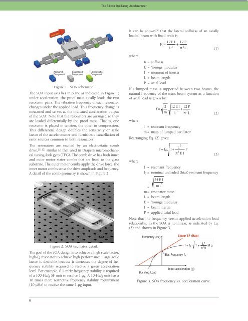
Figure 1. SOA schematic.
The SOA input axis lies in plane as indicated in Figure 1;
under acceleration, the proof mass axially loads the two
resonator pairs. The vibration frequency of each resonator
changes under the applied load. This frequency change is
measured and serves as the indicated acceleration output
of the SOA. Note that the resonators are arranged so they
are loaded differentially by the proof mass. That is, one
resonator is placed in tension, the other in compression.
This differential design doubles the sensitivity or scale
factor of the accelerometer and furnishes a cancellation of
error sources common to both resonators.
The resonators are excited by an electrostatic comb
drive, [1],[2] similar to that used in Draper’s micromechanical
tuning-fork gyro (TFG). The comb drive has both inner
and outer motor stator combs that are fixed to the glass
substrate. The outer motor combs apply the drive force, the
inner motor combs sense the drive amplitude and frequency.
A detail of the comb geometry is shown in Figure 2.
Figure 2. SOA oscillator detail.
The goal of the SOA design is to achieve a high scale-factor,
high-Q resonator to achieve high performance. Large scale
factor is desirable because it decreases the degree of frequency
stability required to resolve a given acceleration
level. For example, 0.1-mHz frequency stability is required
of a 100-Hz/g SF unit to resolve 1 µg. A 10-Hz/g unit has a
10 times more restrictive frequency stability requirement
(10 µHz) to resolve the same 1-µg input.
6
Anchored
Component
Suspended
Component
Electrostatic
Component
The Silicon Oscillating Accelerometer
It can be shown [3] that the lateral stiffness of an axially
loaded beam with fixed ends is:
where:
K = stiffness
E = Young’s modulus
I = moment of inertia
L = beam length
P = axial load
If a lumped mass is supported between two beams, the
natural frequency of the mass-beam system as a function
of axial load is given by:
where:
f = resonant frequency
m = mass of lumped oscillator
Rearranging Eq. (2) gives:
where:
(1)
(2)
(3)
f = resonant frequency
f0 = nominal unloaded (bias) resonant frequency
=
m= resonator mass
L = beam length
E = Young’s modulus
I = beam inertia
P = applied axial load
Note that the frequency versus applied acceleration load
relationship in the SOA is nonlinear, as indicated by Eq.
(3) and shown in Figure 3.
Frequency (Hz)
Buckling Load
Bias Frequency fo
Linear SF (Hz/g)
f = fo
Input acceleration (g)
1 + M g
π2EI L2 Figure 3. SOA frequency vs. acceleration curve.