Decision Models in Skiable Areas - EPFL

Decision Models in Skiable Areas
Semester Project
of
Benjamin Stamm
Directed by:
Dr. Michel Bierlaire
Frank Crittin
Section of Mathematics, EPFL, Lausanne
February 6, 2004
1

CONTENTS 2
Contents
1 Introduction 3
2 Goal of this Semester Project 3
3 Methodology - Discrete Choice Models 4
3.1 Decision Maker . . . . . . . . . . . . . . . . . . . . . . . . . . . . . 4
3.2 Alternatives . . . . . . . . . . . . . . . . . . . . . . . . . . . . . . . 4
3.3 Attributes . . . . . . . . . . . . . . . . . . . . . . . . . . . . . . . . 4
3.4 Random Utility Models . . . . . . . . . . . . . . . . . . . . . . . . . 4
3.4.1 The Deterministic Term . . . . . . . . . . . . . . . . . . . . 5
3.4.2 The Random Term . . . . . . . . . . . . . . . . . . . . . . . 5
3.5 Probit Models . . . . . . . . . . . . . . . . . . . . . . . . . . . . . . 6
3.5.1 Multinomial Probit Model . . . . . . . . . . . . . . . . . . . 6
3.6 Logit Models . . . . . . . . . . . . . . . . . . . . . . . . . . . . . . 7
3.6.1 Binary Logit Model . . . . . . . . . . . . . . . . . . . . . . 7
3.6.2 Multinomial Logit Model . . . . . . . . . . . . . . . . . . . 7
4 Data 8
5 Model of the skiable area of Verbier 8
6 Model of demand in a skiable area 8
6.1 The Lift Model . . . . . . . . . . . . . . . . . . . . . . . . . . . . . 9
6.1.1 The Basic Model . . . . . . . . . . . . . . . . . . . . . . . . 9
6.1.2 Analysis of the Basic Model . . . . . . . . . . . . . . . . . . 11
6.1.3 First approach: Time dependence of ”Minmax” and ”Prot” . . 12
6.1.4 Second Approach . . . . . . . . . . . . . . . . . . . . . . . 14
6.1.5 Interpretation of the Final Model . . . . . . . . . . . . . . . . 16
6.2 The Ski slope Model . . . . . . . . . . . . . . . . . . . . . . . . . . 18
6.3 Implementation in the code . . . . . . . . . . . . . . . . . . . . . . . 18
7 Conclusions 19
8 Future objectives 19

1 INTRODUCTION 3
1 Introduction
This semester project deals with the modelling of a skiable area. This project is in
collaboration with Téléverbier. The behavior of the skiers is modelled and analyzed.
First the theory of Discrete Choice Models is studied in Chapter 3. This Chapter gives
a short introduction to discrete choice models, namely the Logit and Probit Models.
The Chapter 4 describes the data obtained from the part of Téléverbier and Chapter
5 handles about how the skiable area is modelled as a graph. In Chapter 6 a discrete
choice model for the behavior of the skier is developed. For this the theory introduced
in Chapter 3 is used. In fact, the behavior of a skier is divided in two types of decisions.
A first model describes the succession of taken lifts, a second one describes the way
of taken ski slopes between two lifts. Chapter 7 lists the conclusions of this project,
specially of the Lift Model. Chapter 8 is a short preview of possible ways to follow for
future projects.
2 Goal of this Semester Project
The goal of this project is the modelling of the demand in a skiable area. This means to
model the behavior of the skiers. Why do they chose a particular lift and not an other
one? What are the attributes that determine this choice? Is there a difference of the
behavior between a skier with a season ski pass and one with a one day card? This are
a lots of questions that should be treated in this project. The process of work should
take the following steps:
• Introduction to discrete choice models
• Modelling of the area of Verbier
• Modelling of the behavior of the skiers
• Calibration of the parameters of the model
• Implementation in the existing C++ code
• Verification of the model

3 METHODOLOGY - DISCRETE CHOICE MODELS 4
3 Methodology - Discrete Choice Models
This section is an introduction in discrete choice models, and some of them are explained.
Discrete choice models are used when an analyst wants to understand some
human based decisions. Such models are often applied in transportation problems.
3.1 Decision Maker
The decision maker is considered to be an individual, like an person or a group of
persons. In the case of a group, the decision is considered to be one of the whole entire
group.
For example, the decision maker can be a skier in a skiable area which has to decide
between a set of lifts and ski slopes to continue his trip.
3.2 Alternatives
The set of alternatives is called the choice set. This set may be continuous (or not
enumerable), like the time to spend in a restaurant, or discrete, like a set of lifts. In
discrete choice models, only finite choice sets a considered, therefor the name. It is
distinguished between the universal choice set, noted C, and the reduced choice set.
The universal choice set is the set of all possible alternatives that an individual can
chose. The reduced choice set is associated to an particular individual and is the set of
all possible alternatives for this individual in the actual situation.
3.3 Attributes
The attributes are a set of characteristics (an attribute) of the alternatives. They allow
them to be different between them. Each attribute must take a measurable value. It is
distinguished between generic and specific attributes. An generic attribute is one that
can be measured for all alternatives while a specific attribute is one that exist only for
a subset of alternatives.
Example: The decision maker is a skier who has to choose his path. Suppose that
the skier is at the end of a ski slope and that he has to choose the next lift of ski slope.
The universal choice set is the set of all lifts and ski slopes. The reduced choice set is
the set of all lifts and ski slopes that issues from his actual point. An generic attribute
is the length of the lift resp. the ski slope. An specific attribute, defined for each lift,
is the length of the queue of this one. An specific attribute, defined only for the ski
slopes, is the level of difficulty.
3.4 Random Utility Models
In discrete choice models, it exists a map which associates for each alternative (with
the actual values of the attributes) and each individual a value, called utility U i a. It is
a measurement of utility for the decision maker for each alternative. In discrete choice
models, it is always assumed that the analyst don’t posses the complete information. It
is caused to unobserved attributes and measurement errors. So the utility is considered
to be a random variable composed of two components
U i a = V i
a + ε i a
(1)

3 METHODOLOGY - DISCRETE CHOICE MODELS 5
The component V i
a is the deterministic term and discussed in section 3.4.1, whereas
ε i a is the random term and discussed in section 3.4.2. It should be remarked that the
deterministic term is usually of the same form, while the different random terms determines
the kind of Model. Suppose that for all alternatives, the utility is determined.
Then it is supposed that the decision maker chooses the alternatives with the highest
utility. But, because the utility is considered to be a random variable, a probability
Pi C (a) can be associated to each alternative. PiC (a) is the probability that the individual
i will chose alternative a between the set of alternatives C. We have accordingly the
following result:
P i C(a) = P[ U i a = max
b ∈ C U i b ] (2)
Once the random and deterministic terms fixed, we know now how to chose the alternative.
3.4.1 The Deterministic Term
As already mentioned, the deterministic term is a function of the attributes, the alternative
and the decision maker. Usually it is a affine function of the values of the attributes
with one fixed coefficients for each attribute. E.g. the coefficients of two deterministic
functions corresponding to two different alternatives are the same. The constants
are depending of the alternatives, this are the alternative specific constants (ASC). It
is also imageable to introduce a second constant related to an individual or a group of
individuals. The deterministic term has in general the following form:
V i
a = V i
a(x i a) = �
βkx i a(k) + ASCa
(3)
k
where x i a is the vector of all attributes for alternative a and individual i. The scalar
value x i a(k) is the k-th element of the vector x i a and ASCa is the alternative specific
constant related to the alternative a.
3.4.2 The Random Term
This section handles about the random term ε i a and illustrates the principal properties
of it. The random term ε i a is like already mentioned supposed to be a random variable.
Without lost of generality it can be assumed that the mean of ε i a is zero. This property
is illustrated in the following example where the mean of the random variables is
supposed to be different from zero. A decision maker i has the choice between two al-
ternatives 1 and 2 (C = {1, 2}). It is supposed to know the corresponding deterministic
terms V i
1 and V i
2 . Let be m1 and m2 be the means of ε i 1 and ε i 2. Then
P i C(1) = P(U i 1 ≥ U i 2) = P(V i
1 + ε i 1 ≥ V i
2 + ε i 2) = P(V i
1 − V i
2 ≥ ε i 2 − ε i 1) (4)
As next, we define two new random variables εi ′
1 and εi 2
ε i ′
1 = ε i 1 − m1 ε i ′
2
= ε i 2 − m2
It is evident that εi ′ i ′ i
1 resp. ε2 are of mean zero and of the same variance as ε1 resp. εi 2.
Then
P i C(1) = P(V i
1 −V i
2 ≥ ε i ′
2 +m2−ε i ′
1 −m1) = P(V i
1 +m1−V i
2 −m2 ≥ ε i ′ i ′
2 −ε1 ) (6)
′
:
(5)

3 METHODOLOGY - DISCRETE CHOICE MODELS 6
As seen in the previous section the deterministic part includes an alternative specific
constant. The mean of the random variable can be added to the ASC’s. So that in
continuation, the means of the random variables are always supposed to be zero.
The variance can be chosen arbitrary. The argumentation is also illustrated in the
same example as above. Suppose that the random terms ε i 1 resp. ε i 2 are replaced by
αε i 1 resp. αε i 2 with α > 0. Indeed, we have
P(V1 − V2 ≥ αε2 − αε1) = P( 1
α (V1 − V2) ≥ ε2 − ε1) (7)
so that the deterministic term, in fact the coefficients βi, is modified by a factor 1
α .
Usually, two different distributions for the random term are used. They define two
different families of models.
First, the normal or Gauß distribution leads to the family of the Probit models. In
this models, it is assumed that the random terms are normally distributed, with mean
zero. The density function is
fnormal(x) = 1
σ √ 2π
1 x
e− 2 ( σ )2
with σ a positive scale parameter. Indeed, σ 2 is the variance. It is important to notice
that the different ε i a don’t have to be independent and can be correlated.
In the second case, the family of the Logit models, it is assumed that random the
term is independent and identically Gumbel distributed. The density function is
fgumbel(x) = µe −µ(x−η) e −eµ(x−η)
where η is the location parameter and µ the scale parameter. This two families are
explained precisely in the next sections
3.5 Probit Models
3.5.1 Multinomial Probit Model
As mentioned above, the Probit models assumes a normal distribution for the errors.
As consequence and advantage, it allows to capture all correlations between different
alternatives because they are not supposed to be independent. Due to the assumption
that C is finite, the elements of C can be numerated and as consequence C is of the
form C = {a1, a2, . . . , an}. The utility function U i a, ∀a ∈ C, can be written in a vector
form. We define −→ U i , −→ V i and −→ εi componentwise by −→ U i (j) = U i aj , −→ V i (j) = V i
aj and
−→
i i ε (j) = εaj . Then we have
−→
U i = −→ V i + −→ ε i
(10)
where −→ ε i follows a multivariate normal distribution of mean zero and variance covariance
matrix Σ i . So that
PC(k) = P(U i (k) ≥ U i (j)) ∀j ∈ C (11)
The disadvantage of the Probit Models is the normal distribution. Since the analytic
formula of the distribution fonction does not exist, it has to be approximated and causes
a lot of problems.
(8)
(9)

3 METHODOLOGY - DISCRETE CHOICE MODELS 7
3.6 Logit Models
3.6.1 Binary Logit Model
The binary Logit model is a model with two alternatives as in the example above
(C = {1, 2}) where both random terms follow a independent and identically Gumbel
distribution, with same scale and location parameters µ and η. The mean of a Gumbel
distributed random variable is η + γ
µ where γ is the Euler constant.
γ = lim
n�
n→+∞
i=1
1
− ln(n) (12)
n
The variance of a such random variable is π2
6µ 2 . It can be shown that ε = ε2−ε1 follows
a Logistic distribution with location parameter zero and scale parameter µ. The density
function of a Logistic distributed random variable is
so that
flogistic(x) =
µe −µx
(e −µx + 1) 2
(13)
PC(1) = P(V1 − V2 ≥ ε) = flogistic(V1 − V2) (14)
Assuming that both terms are independent and identically distributed leads to that ε is
of mean zero and that
V ar(ɛ) = V ar(ε2 − ε1) = V ar(ε2) + V ar(ε1) = 2π2
6µ 2
It is common to set µ = 1 so that V ar(ɛ) = π2
3 .
3.6.2 Multinomial Logit Model
This model is a generalization of the binary Logit model. As in the binary model, it
is assumed that the random terms are independent and identically Gumbel distributed
with location parameter 0 and scale parameter µ. In this model the decision maker has
more then two alternatives, let C be the set of alternatives. Then C is supposed to be
finite. It can be shown that
PC(a) =
e µVi
�
k∈C eµVk
(15)
a ∈ C (16)
The Multinominal Logit Model satisfy the property of Independence from irrelevant
Alternatives (IIA). This means that the ratio of the probability of two alternatives is
independent of the choice set. Let S and T be such that S ⊆ T ⊆ C and let a1, a2 ∈ S
be two arbitrary alternatives. The property of IIA is satisfied if
PS(a1)
PS(a2) = PT (a1)
PT (a2)
In the case of the Multinominal Logit Model, we have
PS(a1)
PS(a2)
eµV1
= · µV2 e
�
k∈S eµVk
�
k∈S eµVk
= eµV1
�
k∈T
· µV2 e eµVk
�
k∈T eµVk
= PT (a1)
PT (a2)
(17)
(18)

4 DATA 8
View that that the Multinominal Logit Model is a generalization of the Binary Logit
Model, the property of IIA is also satisfied by the Binary Logit Model.
The assumption that the random terms are identically and independent causes problems
with alternatives which are correlated. The red bus/blue bus paradox is illustrated
in [2] or an other example in [1].
4 Data
In this section, the obtained data from the part of Verbier are described. Due to the
system utilizing magnetic cards for the ski-pass, it is possible to draw up a detailed list
about the passages on the lifts. For each passage on a lift, the following information is
given:
• Lift number
• Time
• Date
• Ticket number
• Length of validity of the ticket
• Client category (adult, child,...)
All together it is about 15000 passages in the period between the 8. 11. 2003 and 6.
1. 2004. On average a skier takes about 6 times a lift in a day. Unfortunately, the
passages includes only the sector of Verbier, but the model will be developed for the
sectors Verbier and Mont-Fort. This lack of data in one part of the area will produce
some problems in section 6.1.
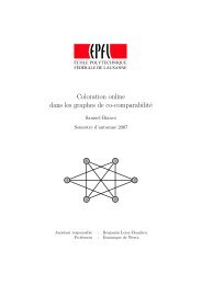
5 Model of the skiable area of Verbier
In this section the area of Verbier and Mont-Fort is modelled. This two sections are
part of whole area ”4 Vallée”. You can find the exact list of the lifts and ski slopes is in
Annexe B. A graphic of the modelled graph is illustrated in Figure 1. At disposal has
been several maps of the area and two detailed papers about the lifts and ski slopes. It
is clear that some simplifications has to be done.
6 Model of demand in a skiable area
In this section, a discrete choice model for the behavior of skiers in an skiable area is
developed.
The movement of a skier in the area is modelled as follows: It exists a first model,
called ”Lift Model” in continuation, that determines the succession of the lifts to take.
The way from the end of a lift to the begin of the next lift is chosen by a second model,
called ”Ski slope Model”. This means for the simulation, that a skier arriving at the
end of a lift chooses first the next reachable lift, then the way to the chosen lift.
In this project we focus on the ”Lift Model”. This is related to the availability of
data. The data is described in Chapter 4. It describes the succession of taken lifts per

6 MODEL OF DEMAND IN A SKIABLE AREA 9
Figure 1: Modelled domain of Verbier
person and day. So it is reasonable to chose the first model also as succession of the
taken lifts of a skier. The second model, the Ski slope model, is neglected in this project
and could be subject in other projects. Because of the unavailability of data of chosen
ski slopes, it is very difficult to develop a such model.
6.1 The Lift Model
In this chapter, the model of choice of the succession of the lifts is described. Once at
the end of a lift arrived, the skier (decision maker) has to choose first the next lift that
he will take. We use for this a Discrete Choice Model as discussed in Chapter 3.
6.1.1 The Basic Model
The Alternatives Let O be the point where the first lift ends and let C be the set of
all lifts. C is the universal choice set. Then we note CO the set of all reachable lifts
starting from O. This is the reduced choice set for a skier who has to take his decision
at the point O. A reachable lift from O is a lift which can be reached from O without
to take an other lift. This means that for all reachable lifts, with D as starting point,
there exists a set of ways, noted WD O . This set WD O contains all possible ways from the
origin to the destination D. WD O is used in the ”Ski slope Model” where an element of
it has to be chosen.
The Attributes Let S be the set of all ski slopes. To each ski slope s ∈ S a cor-
responding level/difficulty ls is defined. The level may be 0 (”blue”), 1 (”red”) or 2
(”black”). May w ∈ WD O be a way from O to D. Then
w = s1 ∪ s2 ∪ . . . ∪ sk si ∈ S ∀i = 1 . . . k (19)
where s1 starts in O and sk ends in D. In the Basic Model, six attributes, which
characterize a lift, are defined. Let LO be the lift ending in O, more precisely the lift

6 MODEL OF DEMAND IN A SKIABLE AREA 10
which the decision maker is ending at. Let also be LD the lift which the decision maker
is considered to chose. The set SLD is the set of ski slopes leaving from the top of LD.
Then the six attributes are:
• The first attribute is the information about the most difficult level of the pistes on
the different ways from O to D:
Maxmax D O = max
w∈W D O
max
i=1,...,k lsi , where w = s1 ∪ s2 ∪ . . . sk (20)
• The second attribute is the minimum level you have to master for skiing form O
to D.
Minmax D O = min
w∈W D O
max
i=1,...,k lsi , where w = s1 ∪ s2 ∪ . . . sk (21)
• The MaxLD attribute is the value of the highest level of the ski slopes leaving
from the top of LD
MaxLD (22)
= max ls
s∈SLD • The MinLD attribute is contrary to the MaxLD attribute the lowest level of ski
slopes leaving from the top of LD.
MinLD
= min ls
s∈SLD • The next attribute is a binary value and it is about the protection against the
weather of the considered lift LD and noted P rotLD . It counts true (”1”) if the
skier is protected against weather on the lift, and false (”0”) otherwise. This
attribute coincide in the particular case of Verbier with the attribute which describes
if the skier have to put off his skis or snowboard. This means that at
every lift with a weather protection you have to put off your skis or snowboard.
(23)
• The last attribute describes the possibility to have a seat or not while using the
lift LD. It is also a binary value and noted SeatsLD.
Note: A such coding of the ski slope level makes the hypothesis that a black ski slope
is considered two times more difficult than a blue one. This hypothesis is accepted in
the Basic Model such as the first approach to improve the Basic Model. The second
Approach respect the fact, that a black ski slope has not to be two times more difficult
than a red one.
The deterministic term In the Basic Model, the deterministic term is only depending
of the alternatives and not from the decision maker itself. Also the constants has been
omitted. As described in section 3.4.1 it has the following form:
Va(xa) = �
βkxa(k) (24)
or with the particular attributes and alternative LD
k
VLD (xLD ) = β1Maxmax D O + β2Minmax D O + β3MaxLD + β4MinLD (25)
+ β5P rotLD + β6SeatsLD (26)
where the same notation is used as above. In further sections, we pose

6 MODEL OF DEMAND IN A SKIABLE AREA 11
Name Value Std err t-test
Max 0.48 0.07 6.80
Maxmax -0.27 0.06 -4.73
Min -2.00 0.18 -11.29
Minmax -1.76 0.07 -26.63
Protection 0.78 0.08 10.15
Sieges 1.05 0.13 8.00
Figure 2: Results of the Basic Model
β1 = Maxmax β2 = Minmax
β3 = Max β4 = Min
β5 = Prot β6 = Seats
The random term In the basic model, a Multinominal Logit Model is used.
Note: In this model (Basic Model), the following hypothesis are supposed:
• Homogeneity: The behavior of all skiers is supposed to be equal. There is no
distinction between different types of skiers.
• Independence of time: The behavior of a skier is supposed the same at 10 am
than at 3 pm.
• A black level ski slope is considered two times more difficult than a red level
one.
6.1.2 Analysis of the Basic Model
The coefficient estimation using the data’s is done with the programm Biogeme 1 . It’s
a programm allowing to estimate the coefficients by maximum of likelihood. It returns
the estimated values of the coefficients, a signification test value for each coefficient
and the correlation between the coefficients. The results of the estimation of the basic
model is shown in Figure 2 where all coefficients satisfies the signification test (t-test).
A further analysis, assuming that the coefficients are random variables, shows that the
hypothesis that Minmax D O and P rotD are random variables can not be rejected. This
is the motivation for the next section and leads to an other model, where these two
attributes are supposed depending on time.
In this paragraph, a explication for the signs of the coefficients is searched
• Maxmax has a negative sign. This would mean that a more difficult way between
to lifts is less attractive. This can not be explained and is the motivation for the
second approach in section 6.1.4
• Minmax has a negative sign, which can be interpreted that the skiers appreciates
more a low level of the minimal difficulty of the ways between to lifts.
• Max has a positive sign. This means that a high level of the attribute ”Max”
(MaxLD = maxs∈SL D ls) is more attractive, which is comprehensible.
1 This is a programme developed by M. Bierlaire which allows to estimate the coefficients of a Multinominal
Logit Model (such as Cross-Nested and GEV-Models)

6 MODEL OF DEMAND IN A SKIABLE AREA 12
• Min has a negative sign. This is also interpretable, in the way that a low ”Min”
(MinLD = mins∈SL D ls) is more attractive.
• Prot has a positive sign and this means that a lift where the skiers are protected
against the weather is more attractive. We have seen that this attribute coincides
with the characteristic to put off the skis. This means that the protection against
the weather is more appreciated by the skiers than the disadvantage to put off the
skis.
• Seats has also a positive sign. A lift where the skiers can sit down is more
attractive than one without the possibility to sit down.
The sign of the coefficient Maxmax can not be interpreted, because the positive sign of
the attribute Max tells us that the skiers like the high-level ski slopes. So it could also
be suspected that the coefficient Maxmax has a positive sign. Or, at least that the both
coefficients have the same sign.
Because the two attributes Manmax D O and P rotD has to be supposed random
variables and because the sign of the coefficient Maxmax can not be interpreted, it is
likely that the Basic Model can be improved. The fact that the attributes Manmax D O
and P rotD are random variables leads to the first approach, the time dependence of
the coefficients Minmax and Prot. This is described in section 6.1.3. The fact, that the
sign of the coefficient Maxmax can not be interpreted in an intuitive way is, as already
mentioned, the motivation of the second approach in section 6.1.4.
6.1.3 First approach: Time dependence of ”Minmax” and ”Prot”
View that the coefficients ”Minmax” and ”Prot” are random variables, a time dependence
of this coefficients is proved. It is assumed that the coefficient in the deterministic
term corresponding to Minmax is
�
T ime
Minmax ·
t0
� λmo
∀ T ime < t0
where the time is measured in minutes and t0 chosen to be 720, what correspond to
noon (starting at midnight). In the afternoon, we have
�
T ime
Minmax ·
t0
� λan
∀ T ime ≥ t0
An example of this function depending of the time is illustrated in Figure 3 where
Minmax is set to 1, λmo and λan to -1.72 and 0.58 respectively. The parameters λmo
and λan can also be estimated by Biogeme. The same approach is done in the case of
the coefficient ”Prot”. This leads to two coefficients µmo and µan. All together, four
additional parameters has to be estimated in this model.
The result of this estimation is illustrated in Figure 4. It can be observed that µmo
is not significant and it reaches the lower bound of −5 which is very unrealistic. The
attribute σan is also not significant. The failure of the t-test means that the hypotheses
of time dependence of the two attributes has to be rejected. You can also remark that
the sign of Maxmax is still negative. This is the reason, why we leave the strategy to
ameliorate the attributes Minmax and Prot. We rather look to change the model that
Maxmax becomes a positive number (Or at least that Max and Maxmax have the same
sign).
(27)
(28)

6 MODEL OF DEMAND IN A SKIABLE AREA 13
0.5
0
−0.5
−1
−1.5
−2
−2.5
−3
550 600 650 700 750
minutes
800 850 900 950
Figure 3: The time depending function with Minmax equals to 1, λmo and λan to -1.72
and 0.58 respectively
Name Value Std err t-test
µmo -5.00 0.00 +Infinity *
µan 2.63 0.77 3.44
λmo -1.72 0.55 -3.13
λan 0.58 0.49 1.20 *
Max 0.48 0.07 6.95
Maxmax -0.29 0.06 -5.05
Min -2.00 0.18 -11.41
Minmax -1.55 0.11 -14.66
Protection 0.48 0.05 9.52
Seats 1.05 0.13 8.18
Figure 4: Results of the model respecting time dependence of Minmax and Prot. The
star (*) means that the corresponding coefficient fails the significance test.

6 MODEL OF DEMAND IN A SKIABLE AREA 14
6.1.4 Second Approach
Figure 5: Procedure of improvement of the Basic Model
In this section we start anew from the Basic Model. First, a neglected problem in
the Basic Model is corrected. The problem is the following: Two lifts succeeding
one another have not a way of ski slopes between. In the Basic Model, it is assumed
that the corresponding attributes Maxmax and Minmax have the fictive values 2 and
0 respectively. This mistake is corrected in this model. For a fixed lift LD, where
the skier is at the end at, and for each succeeding lift LO the attributes Maxmax and
Minmax are eliminated from the deterministic term and a constant is added. This
constant corresponds to the combination of LD and LO. The result is illustrated in
Figure 6. As you can remark, the constants corresponding to ”Col des Gentianes-
Mont-Fort” and ”Jumbo-Mont-Fort” are fixed to zero. This is due to the missing of
data in this part of the domain. There are five constants which are not significant.
More precisely, the hypothesis that this constants are significant has to be rejected. But
because the model will be still developed, the constants will be kept and at the end all
not significant constants will be eliminated (after a possible changing of significance).
As next step, the possibility to avoid the hypothesis that a black ski slope is two
times more difficult than a red one is presented. For each attribute Maxmax D O , MinmaxD O ,
MaxD and MinD, here noted as Attribute D O , two new attributes Attribute redD O and

6 MODEL OF DEMAND IN A SKIABLE AREA 15
Name Value Std err t-test
Attelas 2 Mont-Gelé -29.82 2242151.20 0.00 *
Mayentzet Combe 1 2.97 0.46 6.44
Combe 1 Attelas 2 1.09 0.25 4.27
Combe 1 Combe 2 0.76 0.16 4.77
Combe 1 Attelas 1 0.56 0.16 3.47
Attelas 3 Mont-Gelé -31.34 4773961.90 0.00 *
Col des Gentianes Mont-Fort 0.00 fixed
Lac des Vaux 1 Mont-Gelé -1.97 1.02 -1.93 *
Jumbo Mont-Fort 0.00 fixed
Medran 1 Attelas 2 4.42 1.06 4.17
Medran 1 Combe 2 -27.89 1643908.90 0.00 *
Medran 1 Attelas 1 1.00 1.23 0.82 *
Medran 2 Attelas 2 1.86 0.16 11.50
Medran 2 Combe 2 -2.78 0.42 -6.68
Medran 2 Attelas 1 1.70 0.10 17.03
Attelas 1 Mont-Gelé -2.25 1.02 -2.20
Max 0.10 0.04 2.87
Maxmax -0.79 0.03 -22.72
Min -1.71 0.10 -17.10
Minmax -1.61 0.03 -47.99
Protection 0.43 0.05 9.30
Seats 1.92 0.12 15.70
Figure 6: Results of the model with constants for succeeding lifts. The star (*) means
that the corresponding coefficient fails the significance test.
Attribute black D O
replace the old one. They are defined as follows:
Attribute red D �
1
O =
0
D if AttributeO = 1
otherwise
(red level ski slope)
Attribute black D �
1
O =
0
D if AttributeO = 2
otherwise
(black level ski slope)
This introduces also eight new coefficients (and four are eliminated). The new random
term becomes
VLD (xLD ) = Maxmax redMaxmax redD O
+ Maxmax black · Maxmax black D O
+ Minmax red · Minmax red D O
+ Minmax black · Minmax black D O + Max red · Max redLD
+ Max black · Max blackLD + Min red · Min redLD
+ Min black · Min blackLD + P rot · P rotLD + Seats · SeatsLD
A first analysis shows that the attributes Maxmax red D O , Minmax blackD O , Max redD
and Min blackD are not significant and are eliminated from the model. This Model
leads to the results illustrated in Figure 7. For reason of calculus time the constants has
been reduced. A further analysis of this model, assuming that the attributes are random
variables, shows that in the case of the attributes Max blackD, Minmax red D O ,
Min redD and SeatsD the hypothesis that they are random variables has to be rejected.
For the other two attributes, the hypothesis that they are random variables is
accepted. They are supposed to be normal distributed.

6 MODEL OF DEMAND IN A SKIABLE AREA 16
Name Value Std err t-test
Attelas 2 2.59 0.15 17.45
Mont-Gel -4.66 0.72 -6.50
La Combe 1 3.62 0.46 7.90
La Combe 2 -0.01 0.12 -0.08 *
Mont-Fort 0.00 fixed
Funipace 1.99 0.09 23.26
Max black 0.07 0.04 2.03
Maxmax black -0.89 0.04 -21.99
Min red -1.60 0.10 -15.71
Minmax red -1.71 0.03 -52.23
Protection 0.34 0.04 7.56
Sieges 2.26 0.12 18.77
Figure 7: Results of the model avoiding the hypothesis that a black level ski slope is
two times more difficult than a red one. The star (*) means that the corresponding
coefficient fails the significance test.
Finally, two different types of strategically places were defined. The first type are
places from where a lot of lifts are leaving. The second type are places where a lot of
lifts are ending. In the case of Verbier, the strategically places of the first type are
• ”Les Ruinettes”
• ”La Chaux”
• ”Tortin”
and there are two places of the second type
• ”Les Attelas”
• ”Col des Gentianes”
But the constants corresponding to ”Tortin” and ”Col des Gentianes” are eliminated
because of lack of data in this part of the area. Also the constant corresponding to ”La
Chaux” is eliminate because it fails the significance test and the hypothesis that it exists
has to be rejected.
These all together forms the Final Model, derived from the Basic Model. The
parameters and coefficients of the Final Model are estimated with the large collection
of about 7000 choices from the data. The result is illustrated in Figure 8.
6.1.5 Interpretation of the Final Model
In this section, the result is tried to be interpreted. First the coefficients are interpreted,
then the constants.
Interpretation of the signs of the coefficients
• Max noir (negative):
A lift, where the maximal difficulty of ski slopes leaving from the top is black, is
less attractive than a lift where it is a blue one. This sign can not be interpreted.

6 MODEL OF DEMAND IN A SKIABLE AREA 17
• Min rouge (negative):
Name Value Std err t-test
Attelas D 1.10 0.04 28.13
Col des Gentianes D 0.00 fixed
Attelas 2 Mont-Gelé 0.00 fixed
Mayentzet La Combe 1 5.24 0.56 9.30
La Combe 1 Attelas 2 2.05 0.28 7.31
La Combe 1 La Combe 2 0.55 0.19 2.95
La Combe 1 Funispace 0.84 0.21 4.07
Attelas 3 Mont-Gelé 0.00 fixed
Col des Gentianes Mont-Fort 0.00 fixed
Lac des Vaux 1 Mont-Gelé 0.00 fixed
Jumbo Mont-Fort 0.00 fixed
Médran 1 Attelas 2 0.00 fixed
Médran 1 La Combe 2 0.00 fixed
Médran 1 Funispace 0.00 fixed
Médran 2 Attelas 2 3.24 0.22 15.00
Médran 2 La Combe 2 -3.10 0.42 -7.34
Médran 2 Funispace 2.40 0.19 12.85
Funispace Mont-Gelé 0.00 fixed
La Chaux O 0.00 fixed
Les Ruinettes O 0.76 0.06 12.02
Max black -0.50 0.04 -11.16
Maxmax black -0.76 0.05 -15.00
Min red -1.67 0.10 -16.04
Minmax red -1.92 0.05 -39.42
Protection -0.89 0.10 -8.73
Seats 2.60 0.12 22.36
SigmaMaxmax -1.54 0.10 -15.70
SigmaProt -1.60 0.15 -10.88
Tortin O 0.00 fixed
Figure 8: Results of the Final Model
A lift, where the minimal difficulty of ski slopes leaving from the top is red, is
less attractive than a lift where it is a blue one. This result is logic and could be
expected.
• Maxmax noir:
Random variable of negative mean and large variance. In the average, the maximal
difficulty that the skier can find on the way from the actual place to the next
lift being black is less attractive than a blue difficulty. But this phenomena can
vary a lot between the skiers.
• Minmax rouge (negative):
A level to master for skiing from the actual place to the next lift being red is less
attractive than a blue one. This is also a result that can be expected.
• Protection / Put off the skies:
Random variable of negative mean and large variance. In the average, the fact to
put off the skies disturbs the skiers more than to have a weather protection. But
this phenomena can vary a lot between the skiers.
• Seats (positive):

6 MODEL OF DEMAND IN A SKIABLE AREA 18
A lift on which a skier can sit down is more attractive than in the contrary case.
Interpretation of the constants The constants related to the succession of two lifts
passing par ”Les Ruinettes” are illustrated in Figure 9. Remarkable is the fact that the
combination ”Médran-La Combe 2” is very unattractive and that ”Attelas 2” is for both
preceding possibilities the most attractive choice.
4.00
3.00
2.00
1.00
0.00
-1.00
-2.00
-3.00
-4.00
Attelas 2
6.2 The Ski slope Model
La Combe 2
Funispace
Figure 9: Constants linked to ”Les Ruinettes”
Médran 2
La Combe 1
As mentioned above, the ski slope model is not developed in this project. For the
simulation, a equiprobable model is used. This means that each way from the end of
the actual lift to the begin of the next lift has the same probability to be chosen:
P(alternativei) =
6.3 Implementation in the code
1
# of alternatives
∀i (29)
We have now seen the theory of discrete choice models, have developed a model and
estimated the corresponding coefficients and parameters. Only the implementation in
the code is missing. For this, we use the following algorithm:
Supposing a skier is arriving at the end of a lift, then
Médran 2
La Combe 1

7 CONCLUSIONS 19
• the alternatives, all reachable lifts, are determined
• For all alternatives, the deterministic term of the utility function is determined as
well as the probability that this alternative is chosen. This probability is determined
after formula (16).
• A uniformly random number between 0 and 1 is generated the corresponding
alternative (the next lift) is determined.
• Known the next lift, a way from the actual place to the next lift has to be chosen.
For this anew a uniformly random number between 0 and 1 is generated and the
way is chosen after formula (29) in the preceding section.
Now, the skier knows where to go and the next time he is arriving at the end of a lift,
the same procedure is used.
7 Conclusions
With the Final Model we arrived at a satisfiable model with only significant attributes,
parameters and constants. Some constants are not determinable with the actual set of
data. But, it is probable that with a set covering the whole domain, the remaining constants
could be estimated. The constants seems to be more important than we thought
in the beginning. It is obvious that this model is just a first step to a model describing
a lot of phenomena, observed in a skiable area. For example, our Final Model doesn’t
change the values of the coefficients depending on time. But a model respecting time
dependence is certainly more realistic than the Final Model. The possible improvements
are explained in the next chapter.
8 Future objectives
In this section, I like to suggest possible improvements of the Model. This are some
hints, which has been concretized during this project or for which there was not enough
time to treat it.
• Time dependence: As mentioned in the previous section, it is probable that some
coefficients are depending on time, because the skiers enter the skiable area in the
morning and leave them in the afternoon. View that constants are very important
in this models, I would propose a time dependence of the constants corresponding
to the strategically places.
• Altitude dependence: In my opinion, a higher situated lift is more attractive than
one situated at the bottom of the area. First, because the conditions are often
better in the altitude and second, in the altitude you have a better strategically
position to reach rapidly a wished place in the area. Like in physics, the altitude
is a potential energy. The skier has more freedom to choose his trip starting from
an high situated place. So it is imageable to add an attribute corresponding to the
altitude of the top of the lift in question.
• Socio-economic aspects: It is also probable that a family shows up an other
behavior than a singles skier, a bad skier than a good one, a young skier than an
old one and so on. It would also be interesting if there is a difference between
the behavior of the skiers and the snowborders.

8 FUTURE OBJECTIVES 20
• Dependence of the weather and snow conditions: The attraction of a lift with
weather protection is certainly lower on a beautiful day than otherwise.
• Introduce a attribute that describes the number of alternatives for the next choice.
Aknowledgements
I like to thank L. Perraudin and G. Teicher from Tél´verbier for the collaboration and
their interest in this project as well for the large collection of data which they put at
disposal. I like also to thank M. Bierlaire and F. Crittin who gave me the opportunity
to realize this project.

REFERENCES 21
References
[1] Bierlaire, Michel (1997), Discrete Choice Models: Intelligent Transportation System
Program
[2] Ben-Akiva, M. E. and Lerman, S. R. (1985), Discrete Choice Analysis: Theory
and Application to Travel Demand, MIT Press, Cambridge, Ma.

REFERENCES 22
Appendix A
This graphic defines the points S1 . . . S33.

REFERENCES 23
Appendix B: Detailed information about the area of Verbier
Numéro Description
S1 Verbier
S2 Départ Mayentzet
S3 Fin Mayentzet
S4 Les Ruinettes
S5 Départ LesRuinettes
S6 Fin LesRuinettes
S7 Fin Mdran3
S8 Départ Fontanays
S9 fFantanays
S10 La Chaux
S11 Fin LaChaux2
S12 Départ Attelas3
S13 Attelas
S14 Mont-Gel
S15 Lac des Vaux
S16 Chassoure
S17 Tortin
S18 Col des Gentianes
S19 Mont Fort
S20 Départ Glacier
S21 Fin Glacier
S22 Glacier
S23 Col de Gentianes
S24 La Chaux
S25 La Chaux
S26 La Chaux
S27 La Chaux
S28 La Combe2
S29 La Combe2
S30 La Combe1
S31 Mayentzet
S32 Les Ruinettes
S33 Les Attelas
Figure 10: The nodes of the modelled skiable area of Verbier

REFERENCES 24
Numéro Sommet de départ Sommet finale Niveau Longueur Largeur
P1 S4 S32 B 300 10
P2 S32 S8 B 1300 10
P3 S8 S5 B 1500 10
P4 S32 S5 R 500 100
P5 S5 S30 B 800 10
P6 S30 S3 B 1600 10
P7 S30 S3 R 700 150
P8 S30 S3 N 500 80
P9 S3 S31 B 1000 10
P10 S3 S2 R 700 150
P11 S3 S2 N 500 80
P12 S31 S2 B 900 10
P13 S5 S31 R 1500 100
P14 S2 S1 B 2500 10
P15 S7 S6 R 500 100
P16 S6 S4 R 500 100
P17 S6 S32 R 300 100
P18 S29 S30 R 700 100
P19 S28 S29 R 700 100
P20 S28 S4 R 500 100
P21 S9 S28 R 800 100
P22 S12 S28 R 700 100
P23 S12 S29 N 1200 80
P24 S13 S33 R 1100 100
P25 S13 S12 N 1800 80
P26 S13 S15 B 1000 150
P27 S13 S15 N 600 80
P28 S16 S15 R 800 100
P29 S16 S17 J 3000 100
P30 S20 S17 J 2000 150
P31 S22 S20 R 1100 150
P32 S21 S22 R 400 150
P33 S19 S22 N 1000 150
P34 S22 S18 R 600 150
P35 S18 S20 R 1000 150
P36 S18 S23 R 1500 100
P37 S23 S10 R 1500 100
P38 S23 S24 R 900 100
P39 S24 S10 B 1100 150
P40 S11 S24 B 400 150
P41 S11 S25 R 200 100
P42 S25 S12 R 300 100
P43 S25 S26 R 300 100
P44 S26 S27 R 400 100
P45 S26 S24 R 300 100
P46 S9 S27 R 400 100
P47 S27 S10 R 600 100
P48 S9 S10 B 1500 100
P49 S9 S8 J 1500 100
P50 S33 S12 R 200 100
P51 S33 S25 R 300 100
P52 S16 S13 B 800 100
P53 S14 S17 N 4000 100
P54 S14 S33 N 1000 100
P55 S14 S24 N 1900 100
Figure 11: The pistes of the modelled skiable area of Verbier

REFERENCES 25
Numéro Nom Capacité [personnes/h] Durée Trajet [min] Longueur [m] Vitesse [m/s]
1 Col des Gentianes 800 7’25 3260 10.00
2 Mont-Fort 550 4’10 1425 10.00
3 Jumbo 1125 6’20 2505 10.00
4 Glacier 1 1200 8’94 1502 2.80
5 Glacier 2 1200 9’03 1518 2.80
101 Médran 1 1800 6’45 1645 4.00
102 Médran 2 650 8’30 1620 3.20
103 Médran 3 1000 13’17 1845 2.30
104 Funispace 650 12’00 1950 3.20
105 Attelas 2 2000 4’17 1561 6.00
106 Mont-Gelé 360 3’45 874 9.00
107 Mayentzet 1010 3’55 752 3.20
108 La Combe 1 1400 7’24 1021 2.30
109 La Combe 2 1400 6’45 931 2.30
110 Les Ruinettes 900 4’43 650 2.30
111 Fontanays 1100 8’40 1198 2.30
112 Attelas 3 1100 10’16 1000 2.30
113 La Chaux 1 1300 6’50 820 2.00
114 La Chaux 2 2000 9’20 1120 2.00
116 Lac des Vaux 1 2400 2’21 567 4.50
118 Lac des Vaux 3 1200 5’40 750 2.30
119 Chassoure 1600 6’20 2267 5.00
Nbr de Places par cabine Sommet de départ Sommet d’arrivée Sièges Protection
125 S17 S18 0 1
45 S18 S19 0 1
150 S10 S18 0 1
2 S20 S21 0 0
2 S20 S21 0 0
6 S1 S4 1 1
4 S1 S4 1 1
2 S1 S7 1 0
4 S4 S13 1 1
30 S4 S13 0 1
45 S13 S14 0 1
2 S2 S3 1 0
2 S3 S4 1 0
2 S4 S9 1 0
2 S5 S6 1 0
2 S8 S9 1 0
2 S12 S13 1 0
2 S10 S9 1 0
4 S10 S11 1 0
4 S15 S13 1 0
3 S15 S16 1 0
8 S17 S16 1 1
Figure 12: The lifts of the modelled skiable area of Verbier