The Use and Calibration of the Kern ME5000 Mekometer - SLAC ...
The Use and Calibration of the Kern ME5000 Mekometer - SLAC ...
The Use and Calibration of the Kern ME5000 Mekometer - SLAC ...

Create successful ePaper yourself
Turn your PDF publications into a flip-book with our unique Google optimized e-Paper software.
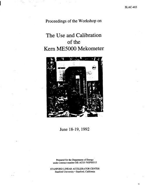
Proceedings <strong>of</strong> <strong>the</strong> Workshop on<br />
<strong>The</strong> <strong>Use</strong> <strong>and</strong> <strong>Calibration</strong><br />
<strong>of</strong> <strong>the</strong><br />
<strong>Kern</strong> <strong>ME5000</strong> <strong>Mekometer</strong><br />
June l&19,1992<br />
Prepared for <strong>the</strong> Department <strong>of</strong> Energy<br />
under contract number DE-AC03-76SFOO515<br />
STANFORD LINEAR ACCELERATOR CENTER<br />
Stanford University � Stanford, California<br />
SLAG4�03
I<br />
--<br />
: . . .<br />
Proceedings <strong>of</strong> <strong>the</strong> Workshop on<br />
<strong>The</strong> <strong>Use</strong> <strong>and</strong> <strong>Calibration</strong><br />
<strong>of</strong> <strong>the</strong><br />
<strong>Kern</strong> <strong>ME5000</strong> <strong>Mekometer</strong><br />
June 1%19,1992<br />
Stanford Linear Accelerator Center<br />
Stanford University<br />
Stanford, California 94309<br />
Edited by Bernard Bell<br />
Survey & Alignment Team, MecbanicaI Engineering Department<br />
September 1992<br />
Prepared for <strong>the</strong> Department <strong>of</strong> Energy<br />
under contract number DE-AC03-76SFOO515<br />
Printed in <strong>the</strong> United States <strong>of</strong> America. Available from tbe National Technical Information<br />
Service, U.S. Department <strong>of</strong> Commerce, 5285 Port Royal Road, Springfield, Virginia 22161.<br />
<strong>SLAC</strong>-403<br />
CONF-9206270<br />
UC-406<br />
(4
--<br />
:<br />
CONTENTS<br />
Participants .............................................................................................................................................. iv<br />
Introductiod ............................................................................................................................................... 7<br />
<strong>ME5000</strong> Operation . . . . . . . . . . . . . . . . . . . . . . . . . . . . . . . . . . . . . . . . . . . . . . . . . . . . . . . . . . . . . . . . . . . . . . . . . . . . . . . . . . . . . . . . . . . . . . . . . . . . . . . . . . . . . . . . . . . . . . . . ............ 9<br />
Bernard Bell, SUC<br />
<strong>ME5000</strong> Test Measurements . . . . . . . . . . . . . . . . . . . . . . . . . . . . . . . . . . . . . . . . . . . . . . . . . . . . . . . . . . . . . . . . . . . . . . . . . . . . . . . . . . . . . . . . . . . . . . . . . . . . . . . . . . . . . . . . . . . 17<br />
Bernard Bell, <strong>SLAC</strong><br />
<strong>ME5000</strong> Data Reduction . . . . . . . . . . . . . . . . . . . . . . . . . . . . . . . . . . . . . . . . . . . . . . . . . . . . . . . . . . . . . . . . . . . . . . . . . . . . . . . . . . . . . . . . . . . . . . . . . . . . . . . . . . . . . . . . . . . . . . . . . 27<br />
Bernard Bell, <strong>SLAC</strong><br />
Variance Component Analysis <strong>of</strong> Baseline Measurements . . . . . . . . . . . . . . . . . . . . . . . . . . . . . . . . . . . . . . . . . . . . . . . . . . . . . . . . . . . . . . . . . . . . . . . 39<br />
Horst Friedsam, <strong>SLAC</strong><br />
<strong>ME5000</strong> Results . . . . . . . . . . . . . . . . . . . . . . . . . . . . . . . . . . . . . . . . . . . . . . . . . . . . . . . . . . . . . . . . . . . . . . . . . . . . . . . . . . . . . . . . . . . . . . . . . . . . . . . . . . . . . . . . . . . . . . . . . . . . . . . . . . . . . . 51<br />
Bernurd Bell, SL4C<br />
<strong>Calibration</strong> <strong>and</strong> <strong>Use</strong> <strong>of</strong> <strong>the</strong> <strong>Mekometer</strong> <strong>ME5000</strong> in <strong>the</strong> Survey <strong>of</strong> <strong>the</strong> Channel Tunnel . . . . . . . . . . . . . . . . . . . . . . . . . . . . . 67<br />
Chris Curtis, CEBAF<br />
. . .<br />
111
1. Ted Lauritzen, LBL<br />
2. Bill Baldock, LBL<br />
3. Robert Rul<strong>and</strong>, SUC<br />
4. Bernard Bell, <strong>SLAC</strong><br />
5. Rick Wilkins, SSC<br />
6. Tom Nurczyck, FNAL<br />
7. Mike Hemmer, BNL 13. John Marsball, FNAL<br />
8. Will Oren, CEBAF 14. Matt Pietryka, SLQC<br />
9. Bernd W<strong>and</strong>, <strong>SLAC</strong> 15. Horst Friedsam, <strong>SLAC</strong><br />
10. Mike Gaydosb, SU C 16. Lassi Kivioja, ANL<br />
11. Chris Curtis, sue 17. Byung-Guk Kim, PLS<br />
12. Merrick Penicka, ANL<br />
V
Argonne National Laboratory<br />
9700 South Cass Road,<br />
Argonne, IL 60439<br />
BNL<br />
Brookbaven National Laboratory<br />
Upton, NY 11973-5000<br />
PARTICIPANTS<br />
CEBAF<br />
Continuous Electron Beam Accelerator Facility<br />
12000 Jefferson Avenue,<br />
Newport News, VA 23606<br />
F’NAL (Fermllab)<br />
Femi National Accelerator Laboratory<br />
P.O. Box 500<br />
Batavia, IL 60510<br />
LBL<br />
Lawrence Berkeley Laboratory<br />
1 Cyclhron Road,<br />
Berkeley, CA 94720<br />
PLS<br />
Pobang Light Source<br />
P.O. Box 125<br />
Pobang<br />
Rep. <strong>of</strong> Korea 790-600<br />
<strong>SLAC</strong><br />
Stanford Linear Accelerator Center,<br />
P.O. Box 4349,<br />
Stanford, CA 94309<br />
ssc<br />
Superconducting SupexCollider<br />
2550 Beckleymeade Ave,<br />
Dallas, lX 75237<br />
-- iv<br />
Lussi Kivioja<br />
Merrick Penicka<br />
Mike Hemmer<br />
Chris Curtis<br />
Will Oren<br />
John Marshall<br />
Tom Nurczyck<br />
Bill Baldock<br />
Ted Luuritzen<br />
Byung-Guk Kim<br />
Bernard Bell<br />
Horst Friedsam<br />
Mike Gaydosh<br />
Matt Pietryka<br />
Roben Rulund<br />
Bemd W<strong>and</strong><br />
Rick Wilkins
-<br />
INTRODUCTION<br />
Wben it was introduced in 1986 <strong>the</strong> <strong>Kern</strong> <strong>ME5000</strong> <strong>Mekometer</strong> immediately attracted attention from<br />
<strong>the</strong> survey groups <strong>of</strong> accelerator laboratories around <strong>the</strong> world. This interest was generated not only<br />
because <strong>the</strong> ‘<strong>ME5000</strong> <strong>of</strong>fered bigber accuracy than any o<strong>the</strong>r distance measuring instrument on -<strong>the</strong><br />
market, but also because, unlike previous instruments, its measuring range extended down to just a few<br />
meters, thus opening up <strong>the</strong> wbole realm <strong>of</strong> accelerator housings to high-accuracy EDM measurements.<br />
Abbougb <strong>Kern</strong> quoted a range <strong>of</strong> 20-8000 m, s<strong>of</strong>tware was quickly made available to extend <strong>the</strong><br />
measurement range below 20 m (<strong>the</strong> PROMEKO program developed by <strong>the</strong> Technical University <strong>of</strong><br />
Munich).<br />
In 1988-89 three DOE laboratories (CEBAF, FNAL <strong>and</strong> LBL) acquired instruments. ‘Since none <strong>of</strong><br />
<strong>the</strong>se laboratories bad equipment to calibrate <strong>the</strong>se instruments whereas <strong>SLAC</strong> did, extensive tests were<br />
made witb all three instruments at <strong>SLAC</strong> in 1989.’ When four o<strong>the</strong>r laboratories initiated tbe<br />
procurement process in tbe second half <strong>of</strong> 1991 to buy <strong>the</strong>ir own machines, plans were set in motion to<br />
make a full series <strong>of</strong> test measurements with all DOE instruments, bringing <strong>the</strong>m to <strong>SLAC</strong> one at a time.<br />
Measurements commenced in January 1992 when <strong>the</strong> LBL, FNAL <strong>and</strong> CEBAF insmmrents were<br />
measured in quick succession. Tbe ANL <strong>and</strong> BNL instruments, both new, followed in February <strong>and</strong><br />
March. In June <strong>SLAC</strong> received its own instrument <strong>and</strong> measurements began right away.<br />
As what was to have been <strong>the</strong> culmination <strong>of</strong> this project, a workshop was held at <strong>SLAC</strong> in mid-June<br />
to discuss tbe results. 16 people from 7 DOE laboratories attended as well as one representative from <strong>the</strong><br />
Pohang Light Source in Korea (see <strong>the</strong> list <strong>of</strong> participants on p. iv). By this time measurements were<br />
complete for five instruments <strong>and</strong> mostly complete for a sixth (<strong>the</strong> <strong>SLAC</strong> instrument). This volume is <strong>the</strong><br />
for@ record <strong>of</strong> tbesix papers that were presented during <strong>the</strong> two days <strong>of</strong> <strong>the</strong> workshop. Tbe first paper<br />
covers <strong>ME5000</strong> Operation - how <strong>the</strong> instrument works. <strong>The</strong> second describes <strong>the</strong> measurements that were<br />
made at <strong>SLAC</strong> with eacbinstrument. Data analysis is described in <strong>the</strong> third <strong>and</strong> fourth papers, <strong>and</strong> <strong>the</strong><br />
results are presented in <strong>the</strong> fifth paper. <strong>The</strong> final paper is a special invited paper commissioned from<br />
Chris Curtis <strong>of</strong> CEBAF who spent three years (1987-89) working with a <strong>ME5000</strong> on <strong>the</strong> Channel Tunnel<br />
project in Engl<strong>and</strong>.<br />
<strong>The</strong> Workshop proved not to be tbe culmination <strong>of</strong> <strong>the</strong> project for two more instruments were<br />
measured in August - <strong>the</strong> two SSC instruments. <strong>The</strong> workshop papers presented in this volume have heen<br />
updated to incorporate <strong>the</strong>se results. <strong>The</strong> baseline measurements for tbe <strong>SLAC</strong> instrument have not heen<br />
completed <strong>and</strong> sufficient time has elapsed that <strong>the</strong>y must be started afresh, something that is not feasible<br />
in <strong>the</strong> next few months. <strong>The</strong>se updated proceedings <strong>the</strong>refore represent <strong>the</strong> culmination <strong>of</strong> this project to<br />
test tbe <strong>ME5000</strong> instruments at use in each DOE laboratory.<br />
<strong>SLAC</strong><br />
September 22,1992<br />
’ T.W. Copel<strong>and</strong>-Davis, Can <strong>the</strong> <strong>Kern</strong> <strong>ME5000</strong> Mekometa Replace Invar Measuremnts? Rcpulu<br />
Machines, Procedings <strong>of</strong> <strong>the</strong> First Intemational Wonkshop on AccelcrtirAlignmmt, <strong>SLAC</strong>, July 31 - August 2, 1989, pp. 171-183.<br />
7<br />
d Test ~mmnts witi l’hree
I<br />
--<br />
:<br />
<strong>ME5000</strong> OPERATION<br />
Bernard Bell, <strong>SLAC</strong><br />
1. BASIC PRICIPLES OF EDM<br />
<strong>The</strong> basic principle behind all EDM instruments is <strong>the</strong> same: a beam <strong>of</strong> known frequency F is sent to<br />
a target <strong>and</strong> reflected back to <strong>the</strong> instrument. This’round-trip distance 20 inc1udes.a.n integral number <strong>of</strong><br />
wavelengths m h plus a fractional part <strong>of</strong> a wavelength f L<br />
W = mX+fh (1)<br />
<strong>The</strong> desired result is <strong>the</strong> oneway distance D not <strong>the</strong> round-trip distance 20. It is usual to describe<br />
this one-way distance D as containing <strong>the</strong> same number m <strong>of</strong> half-wavelengths U2,<br />
h h<br />
D= mpfz (2)<br />
<strong>The</strong> precise value <strong>of</strong> this half-wavelength h/2, also known as <strong>the</strong> eflective wavelength, depends upon<br />
<strong>the</strong> refractive index <strong>of</strong> <strong>the</strong> air through which <strong>the</strong> beam travels, nb<br />
3L conk<br />
---<br />
2- 2F<br />
in which c, is <strong>the</strong> velocity <strong>of</strong> light in vucuo, 299792458 ms-‘.<br />
Three methods have been used to find m <strong>and</strong> f <strong>and</strong> thus find <strong>the</strong> distance D.<br />
1.1. Phase Resolution<br />
Most infra-red EDM instruments, such as <strong>the</strong> DM503, determine <strong>the</strong> fractional part f by measuring<br />
<strong>the</strong> phase angle A$ between <strong>the</strong> outgoing beam <strong>and</strong> <strong>the</strong> return beam, (4) <strong>and</strong> Fig. 1.<br />
AGVRE 1. Distance &termination by phase resolution<br />
Such an approach, though <strong>the</strong> cheapest <strong>and</strong> simplest, introduces cyclic error into <strong>the</strong><br />
measurements. To find <strong>the</strong> value <strong>of</strong> m, <strong>the</strong> measurement is repeated using several predefined frequencies.<br />
(3)
--<br />
1.2. Path Length Modification<br />
<strong>ME5000</strong> Operation<br />
<strong>The</strong> <strong>Kern</strong> ME3000 <strong>Mekometer</strong> eliminates <strong>the</strong> fractional part f by changing <strong>the</strong> patb distance D until<br />
<strong>the</strong> phase difference is zero, indicating an integral number <strong>of</strong> half-wavelengths, (5) <strong>and</strong> Fig. 2.<br />
D+6D = mf (5)<br />
< D .f SD+<br />
< m.?J2 ><br />
FIGURE 2. Distance determination by changing <strong>the</strong> parh lengrh<br />
As in <strong>the</strong> first approach, m is found by repeating <strong>the</strong> measurement using several predefmed<br />
frequencies.<br />
1.3. Frequency Modification<br />
<strong>The</strong> <strong>Kern</strong> MESO& <strong>Mekometer</strong> also eliminates <strong>the</strong> fractional part f, but by using a different method.<br />
<strong>The</strong> frequency is changed until a zero phase difference is obtained, (6) <strong>and</strong> Fig. 3.<br />
?b<br />
= m.-<br />
D 2<br />
(6)<br />
< D ><br />
FIGURE 3. Distance determination by changing <strong>the</strong> frequency<br />
<strong>The</strong> value <strong>of</strong> m is found in a manner different from <strong>the</strong> frrst two approaches. <strong>The</strong> frequency is<br />
increased in small steps until a zero phase difference is again detected, at which frequency <strong>the</strong> path<br />
contains m+l <strong>of</strong> <strong>the</strong>se new half-wavelengths X1/2,<br />
D = (m+l)$ (7)<br />
<strong>The</strong>se two frequencies provide sufficient information to resolve m <strong>and</strong> thus <strong>the</strong> distance.<br />
10
--<br />
<strong>The</strong> second <strong>and</strong> third approaches afford <strong>the</strong> ME3000 <strong>and</strong> ME5ooO greater accuracy for two reasons:<br />
a) <strong>The</strong> null condition or zero point at which <strong>the</strong>re is no phase difference can be located with greater<br />
accuracy than a defmite phase difference can be measured.<br />
b) Since <strong>the</strong> phase diierence is always <strong>the</strong> same <strong>the</strong>re is no cyclic error.<br />
2. THE MODULATION SIGNAL<br />
<strong>The</strong> carrier beam is a HeNe laser (Class II, 1 mW) <strong>of</strong> 632.8 run wavelength. Onto this is<br />
superimposed <strong>the</strong> reference signal which is polarization modulated at a frequency <strong>of</strong> ~500 MHz, giving<br />
an effective wavelength (A/2 = c12F) <strong>of</strong> 30 cm. <strong>The</strong> nominal range <strong>of</strong> <strong>the</strong> modulator crystal is 460 - 510<br />
MHz. Within this range <strong>the</strong> modulation b<strong>and</strong>width <strong>of</strong> <strong>the</strong> modulation is a nominal 15 MHz. <strong>The</strong> quartz<br />
oscillator from which <strong>the</strong> modulation signal is derived is compensated for temperature effects to ensure<br />
high accuracy.<br />
Before a measurement can be made <strong>the</strong> instrument must perform a modulator calibration using<br />
function SF141. <strong>The</strong> power intensity output <strong>of</strong> <strong>the</strong> modulator is measured at 75 intervals throughout <strong>the</strong><br />
entire nominal range 460 - 510 MHz. From this calibration <strong>the</strong> upper <strong>and</strong> lower limits <strong>of</strong> <strong>the</strong> normal<br />
(nominal 15 MHz) <strong>and</strong> extended (nominal 30 MHz) b<strong>and</strong>widths are determined.<br />
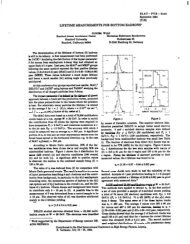
<strong>The</strong> plot <strong>of</strong> power intensity against fkquency is tamed <strong>the</strong> characteristic curve. Fig. 4 shows <strong>the</strong><br />
nominal characteristic curve as shown in <strong>the</strong> <strong>Kern</strong> literature. ‘I&e actual measured curves can differ<br />
substantially from this nominal shape. Fig. 5 shows <strong>the</strong> measured curves for two instruments. <strong>The</strong> reason<br />
for <strong>the</strong> discrepancy in shapes is not known.<br />
-<br />
60<br />
I<br />
I<br />
I<br />
I<br />
I<br />
I<br />
I<br />
I<br />
I<br />
I<br />
I<br />
r<br />
mear 14 a2 w-k<br />
L<br />
470 4s i;-<br />
490<br />
Figure 4. Nominal Characferisfic Curve<br />
11<br />
I<br />
I<br />
I<br />
\<br />
)J-<br />
I<br />
I<br />
I<br />
I<br />
I<br />
I<br />
I<br />
L<br />
510 MM
-<br />
0<br />
/<br />
I-<br />
<strong>ME5000</strong> Operation<br />
4&l 470 480 4Kl SW 510<br />
fmqwncy (MHzl<br />
Figure 5. Actual Characteristic Curves for Instruments 357037 <strong>and</strong> 357081<br />
For short-distance measurements, below 20 m, <strong>the</strong> normal 15 MHz b<strong>and</strong>width is insufficient (for<br />
reasons explained below), so <strong>the</strong> intensity threshold is reduced to 75% <strong>of</strong> maximum to give a wider<br />
b<strong>and</strong>width, nominally 30 MHz. In practice, this b<strong>and</strong>width is dependent upon <strong>the</strong> characteristics <strong>of</strong> <strong>the</strong><br />
individual crystal, <strong>and</strong> has been found to vary in <strong>the</strong> range 18 - 29 MHz. Table 1 shows <strong>the</strong> normal <strong>and</strong><br />
extended b<strong>and</strong>widths for <strong>the</strong> two instruments shown in Fig. 5.<br />
357037 (LBL)<br />
357081. (SSC)<br />
3.1 Normal Mode<br />
Table 1. Modulation b<strong>and</strong>width <strong>of</strong> instruments 357037 <strong>and</strong> 357081<br />
NORMAL. EXTENDED<br />
Range (MHz) B<strong>and</strong>width Rarqe (MHz) B<strong>and</strong>width<br />
472.112 - 486.915 14.803 465.383 - 494.644 28.261<br />
472.785 - 486.915 14.130 469.420 - 490.280 20.859<br />
3. RESOLVING THE DISTANCE<br />
<strong>SLAC</strong>’s field measurement <strong>and</strong> data collection program ME5COO.BAS mimics <strong>the</strong> operation <strong>of</strong> <strong>the</strong><br />
onboard program in <strong>the</strong> ME5OOO’s EPROM for <strong>the</strong> measurement <strong>of</strong> distances in <strong>the</strong> normal operating range<br />
<strong>of</strong> <strong>the</strong> instrument, 20 - 8000 m.<br />
3.1.1. Calculation <strong>of</strong> distance from frequency<br />
Starting at <strong>the</strong> lower end <strong>of</strong> <strong>the</strong> b<strong>and</strong>width an upward sweep is made until a frequency F1 is found at<br />
which <strong>the</strong> phase difference is zero. This nodal point occurs when <strong>the</strong>re is an integer number ml <strong>of</strong> half-<br />
wavelengths along <strong>the</strong> measurement path. <strong>The</strong> sweep is continued until a second nodal point is found at<br />
frequency Fl,.+ at which <strong>the</strong>re are ml+1 half-wavelengths. <strong>The</strong> distance can be determined from <strong>the</strong><br />
frequency difference FM-FI, (S-10).<br />
12<br />
.
:<br />
- _<br />
ml<br />
=<br />
Anti<br />
co<br />
D<br />
mr+l = 2Fune D<br />
co<br />
D<br />
co<br />
= 2n&(Fu - Fl)<br />
<strong>The</strong> frequency diierence FM - Fl is proportional to <strong>the</strong> distance, Table 2.<br />
Table 2. Correlation betweenfrequency &fference <strong>and</strong> distance<br />
I Distance<br />
m<br />
I 5<br />
10<br />
20<br />
50<br />
100<br />
1000<br />
8000<br />
h-F1<br />
MHz<br />
29.971<br />
14.985<br />
1.493<br />
2.997<br />
1.499<br />
0.150<br />
0.019<br />
- <strong>The</strong> range limitations <strong>of</strong> <strong>the</strong> <strong>ME5000</strong> can be understood from Table 2. <strong>Kern</strong> specifies a working<br />
range <strong>of</strong> 20 - 8000 m. Within this range all distances can be measured unambiguously in st<strong>and</strong>-alone<br />
mode using <strong>the</strong> s<strong>of</strong>tware programmed into <strong>the</strong> EPROM in tbe instrument. <strong>The</strong> upper limit <strong>of</strong> 8 km is<br />
imposed by <strong>the</strong> minimum step size in <strong>the</strong> coarse <strong>and</strong> fine search routines. <strong>The</strong> lower limit <strong>of</strong> 20 m is<br />
imposed by <strong>the</strong> requirement <strong>of</strong> finding two adjacent nodal points within tbe b<strong>and</strong>width <strong>of</strong> 15 MHz.<br />
Distances above 8 km <strong>and</strong> below 20 m can be measured only using special s<strong>of</strong>tware.<br />
If possible, more than two nodal points are used in order to improve <strong>the</strong> accuracy. Up to four nodal<br />
points are located, Fig. 6.<br />
Q<br />
phase -<br />
ditterancs<br />
I<br />
I<br />
Fl FlA F2 F3<br />
+DF+<br />
- Modulator Range -<br />
Figure 6. Location <strong>of</strong> nullpoints<br />
I<br />
Frequency<br />
1. F1, <strong>the</strong> first nodal point found in <strong>the</strong> upward sweep from tbe lower end <strong>of</strong> <strong>the</strong> b<strong>and</strong>width.<br />
2. FM, <strong>the</strong> nodal point adjacent to Fl. <strong>The</strong> approximate locations <strong>of</strong> F2 <strong>and</strong> F3 are <strong>the</strong>n calculated<br />
using <strong>the</strong> frequency interval between nodes, FM - Fl.<br />
3. F2, <strong>the</strong> nodal point approximately in <strong>the</strong> center <strong>of</strong> <strong>the</strong> b<strong>and</strong>width<br />
4. F3, <strong>the</strong> nodal point nearest <strong>the</strong> upper limit <strong>of</strong> <strong>the</strong> b<strong>and</strong>width.<br />
If <strong>the</strong>y exist, Fl,- F2, <strong>and</strong> F3 are used for <strong>the</strong> final distance calculation. If only three frequencies are<br />
13<br />
(8)
<strong>ME5000</strong> Operation<br />
found, F2 = FL.+ For a few distances in <strong>the</strong> range 20-25 m only two frequencies, F1 <strong>and</strong> F3, are found.<br />
At ‘each nodal point <strong>the</strong> frequency is determined by a coarse measurement followed by a fine<br />
measurement. _<br />
3.13. Coarse search in normal mode<br />
Using <strong>the</strong> onboard coarse search function (SF144) <strong>the</strong> Frequency is increased by predefmed<br />
increments, starting from <strong>the</strong> lower end <strong>of</strong> <strong>the</strong> b<strong>and</strong>width, until a zero point (zero phase difference) is<br />
found. Each zero point is indicated by a reduction in <strong>the</strong> light intensity falling on <strong>the</strong> detector diode in <strong>the</strong><br />
instrument. When <strong>the</strong> outgoing <strong>and</strong> return signals are exactly in phase no light falls on <strong>the</strong> diode, Fig. 7.<br />
Light<br />
Intensity<br />
3.1.3. Fine search in normal mode<br />
,,..- ------- . .._.,____ ------. .,.. ohsrscterlstic curve<br />
,..’ -._,____,,.,_.._...-. /----<br />
,,’<br />
'i<br />
..z<br />
\<br />
i'<br />
!..<br />
FIGURE 7. Light intensity at <strong>the</strong> receiver diode<br />
Frequency<br />
<strong>The</strong> onboard function SF145 performs <strong>the</strong> fine search routine. Due to background noise it is difficult<br />
to pick up <strong>the</strong> minimum signal itself. Instead, <strong>the</strong> instrument superimposes a 2 kHz wobbler frequency.<br />
<strong>The</strong> amplitude <strong>of</strong> this signal is 9~6.7 kHz for high range (>500 m) <strong>and</strong> i35 kHz for low range (20 - 500<br />
m). When <strong>the</strong> oscillation <strong>of</strong> this 2 kHz signal covers <strong>the</strong> zero point itself it produces a 4 kHz signal. This<br />
means that <strong>the</strong> coarse search must locate <strong>the</strong> zero point to within half <strong>the</strong> b<strong>and</strong>width <strong>of</strong> this wobbler<br />
frequency. If <strong>the</strong> mean frequency does not exactly coincide with <strong>the</strong> zero point a 2 kHz signal is also<br />
produced, Fig. 8(a). When <strong>the</strong> mean frequency does coincide with <strong>the</strong> zero point this 2 kH.z signal<br />
disappears, Fig. S(b). <strong>The</strong> wobbler frequency is adjusted in steps <strong>of</strong> 162 Hz until <strong>the</strong> zero point is located.<br />
This smallest step <strong>of</strong> 162 Hz is equivalent to a change in wavelength <strong>of</strong> 0.1 p.<br />
(a) Non-tuned case<br />
(b) Tuned case<br />
sea table<br />
FIGURE 8. Determination <strong>of</strong> <strong>the</strong> zero point using a 2 kHz wobbler signal<br />
14
:<br />
iUE5LH.W Operation<br />
<strong>The</strong> precise frequency <strong>of</strong> <strong>the</strong> zero point is <strong>the</strong> weighted average <strong>of</strong> five sets <strong>of</strong> 256 individual<br />
measurements (a total <strong>of</strong> 1280 individual determinations <strong>of</strong> <strong>the</strong> zero point).<br />
3.2. Short Distance Measurements<br />
In st<strong>and</strong>-alone mode using its onboard program, measurements can be made only in <strong>the</strong> normal<br />
operating range 20 - 8000 m. For measurement above 8 lan or below 20 m, an external computer must<br />
guide <strong>the</strong> instrument through <strong>the</strong> necessary measurement steps. <strong>The</strong> <strong>SLAC</strong> program ME5OOO.BAS<br />
incorporates <strong>the</strong> necessary routines for measurements below 20 m, but not for measurement above 8 km as<br />
<strong>the</strong> need has never arisen.<br />
For distances below 20 m a different search method is used, as described below.<br />
3.2..1 Coarse search in short-distance mode<br />
Ra<strong>the</strong>r than use <strong>the</strong> coarse search function (SF144) in <strong>the</strong> <strong>ME5000</strong> Crp, a coarse search is made under<br />
<strong>the</strong> control <strong>of</strong> <strong>the</strong> ME5ooO program. In response to code 68, <strong>the</strong> <strong>ME5000</strong> returns <strong>the</strong> phase position $ in<br />
hexadecimal in <strong>the</strong> range 00 - FF. 7F indicates zero phase, but is ambiguous: it indicates a phase<br />
diierence <strong>of</strong> ei<strong>the</strong>r 0 or x. On earlier EDM instruments with a manual phase meter (e.g., ME3000),<br />
whe<strong>the</strong>r <strong>the</strong> signals are in phase or exactly out <strong>of</strong> phase is determined by <strong>the</strong> direction in which <strong>the</strong> needle<br />
is moving. Similarly, in <strong>the</strong> <strong>ME5000</strong> <strong>the</strong> two signals are in phase if <strong>the</strong> phase decreases with decreasing<br />
frequency or increases with increasing frequency for slight changes in frequency around <strong>the</strong> null point.<br />
Fig. 9 shows <strong>the</strong> phase signal across <strong>the</strong> entire extended b<strong>and</strong>width for a distance <strong>of</strong> 20m. <strong>The</strong>re are four<br />
nodes, two in <strong>the</strong> normal b<strong>and</strong>width <strong>and</strong> two in <strong>the</strong> extended b<strong>and</strong>width. <strong>The</strong> transition from + = 00 to<br />
Q = FF covers just a few kHz.<br />
FF --<br />
Phase CI-<br />
00<br />
� Exactly in phase<br />
� Exactly out <strong>of</strong> phase<br />
Extended B<strong>and</strong>width ->I<br />
<strong>ME5000</strong> Operation<br />
Al = wavelength for frequency Ft<br />
D = approx. distance<br />
AiE = addition constant<br />
D = rnlhl-ADC (13)<br />
Short distance measurements below 20 m form <strong>the</strong> bulk <strong>of</strong> <strong>the</strong> work performed with <strong>the</strong> <strong>ME5000</strong> at<br />
particle accelerators. <strong>The</strong> majority <strong>of</strong> <strong>the</strong>se distances are already known to within a millimeter or so. <strong>The</strong><br />
<strong>ME5000</strong> program provides a feature to enter a pre-known distance. This distance must be sufficiently<br />
close to <strong>the</strong> actual distance that <strong>the</strong> wobbler kq~ency falls over <strong>the</strong> zero point during <strong>the</strong> coarse search<br />
(see Fig. 8 <strong>and</strong> description). <strong>The</strong> entry <strong>of</strong> a valid preknown distance produces a considerable saving in<br />
time.<br />
16<br />
(11)<br />
(12)
--<br />
-<br />
<strong>ME5000</strong> TEST MEASUREMENTS<br />
Bernard Bell, <strong>SLAC</strong><br />
1. ERRORS IN EDM INSTRUMENTS<br />
<strong>Calibration</strong> <strong>of</strong> EDM instruments is necessary in order to determine three different types <strong>of</strong> error: -<br />
<strong>of</strong>fset error, cyclic error <strong>and</strong> scale error.<br />
1.1. Offset error<br />
<strong>The</strong> largest error <strong>and</strong> <strong>the</strong> one that must always be determined prior to any measurement is what is<br />
known variously as <strong>the</strong> zero <strong>of</strong>fset, <strong>the</strong> <strong>of</strong>fset error, or <strong>the</strong> instrument constant. This is a constant error<br />
caused by <strong>the</strong> inability to perfectly align <strong>the</strong> optical <strong>and</strong> electronic components to <strong>the</strong> mechanical center <strong>of</strong><br />
<strong>the</strong> instrument. Fortunately, as well as being <strong>the</strong> largest error, <strong>the</strong> <strong>of</strong>fset error is <strong>the</strong> easiest to determine.<br />
<strong>The</strong> simplest determination can be made by measuring all three distances between three colinear points<br />
(Fig. 1).<br />
A B c<br />
0 0<br />
Sob Sbc<br />
-Sbc -<br />
FIGURE I. Simple methodfor determining <strong>the</strong> zero <strong>of</strong>fset<br />
Each <strong>of</strong> <strong>the</strong> three distance measurements (s AB, s,,, , sBc) contains <strong>the</strong> true distance plus <strong>the</strong> zero <strong>of</strong>fset,<br />
a,. <strong>The</strong> <strong>of</strong>fset is <strong>the</strong>refore easily calculated,<br />
Eo = SK - (s, + SBC) (1)<br />
<strong>The</strong> addition constant <strong>of</strong> each <strong>ME5000</strong> is determined in Switzerl<strong>and</strong> prior to shipping <strong>the</strong> unit. <strong>The</strong><br />
value <strong>of</strong> <strong>the</strong> <strong>of</strong>fset is set on rotary switches in <strong>the</strong> instrument. <strong>The</strong> value set on <strong>the</strong>se switches is not <strong>the</strong><br />
actual value but that value subtracted from 20 cm. It is set to an accuracy <strong>of</strong> 0.1 mm.<br />
1.2. Cyclic error<br />
LBL<br />
Fermilab<br />
CBBAF<br />
Argonne<br />
Brookhaven<br />
<strong>SLAC</strong><br />
Tab& 1. MESo Addition constants<br />
Serial number Switch settings<br />
351031 G1<br />
357046 5.78<br />
357036 5.77<br />
357086 5.74<br />
357088 5.84<br />
357089 5.80<br />
Addition constant<br />
0.1422<br />
0.1423<br />
0.1426<br />
0.1416<br />
0.1420<br />
Cyclic error affects only those instruments that use phase resolution - this includes most <strong>of</strong> <strong>the</strong> infra-<br />
red instruments such as <strong>the</strong> DM503, but not <strong>the</strong> <strong>ME5000</strong>. Since <strong>the</strong> <strong>ME5000</strong> always locates a constant<br />
zero phase difference it is immune to cyclic error.<br />
17 .
I<br />
--<br />
-<br />
:<br />
1.3. Scale error<br />
<strong>ME5000</strong> Test Measurements<br />
Scale error is due to an error in <strong>the</strong> frequency <strong>of</strong> modulation <strong>of</strong> <strong>the</strong> carrier beam. Determination <strong>of</strong><br />
<strong>the</strong> error <strong>the</strong>refore consists in measuring <strong>the</strong> emitted Bequency <strong>and</strong> comparing this against <strong>the</strong> frequency<br />
<strong>the</strong> instrument thinks it is using. <strong>The</strong> method used to do this is described below in Section 4 on<br />
Frequency Measurements.<br />
Three series <strong>of</strong> test measurements were conducted in order to evaluate <strong>the</strong> behavior <strong>of</strong> each<br />
instrument: baseline measurements, interferometer measurements <strong>and</strong> frequency measurements. <strong>The</strong>se<br />
tests am described below.<br />
2.1. <strong>The</strong> <strong>SLAC</strong> Baseline<br />
2. BASELINE MEASUREMENTS<br />
<strong>The</strong> <strong>SLAC</strong> baseline was constructed in mid-1985 along <strong>the</strong> south side <strong>of</strong> <strong>the</strong> Linac. Twenty pillars<br />
(BOl - B20) were erected (Table 2). <strong>The</strong> baseline runs nearly due east-west from BOl in <strong>the</strong> west at Sector<br />
O-O above <strong>the</strong> Linac injector to B20 in <strong>the</strong> east at Sector 21-2.<br />
Each pillar is a 1-ft diameter reinforced concrete post, poured in situ, that protrudes 3 ft above ground<br />
<strong>and</strong> descends 4 ft beneath ground. Each pillar is topped with a CERN socket. Most <strong>of</strong> <strong>the</strong> pillars are on<br />
<strong>the</strong> grass verge beside <strong>the</strong> access road.<br />
<strong>The</strong> linac slopes downward from <strong>the</strong> west end at a slope <strong>of</strong> approximately 0.005 (0.3”). <strong>The</strong> intention<br />
was to set out <strong>the</strong> baseline in such a manner that <strong>the</strong> CERN sockets atop <strong>the</strong> pillars follow a geometrical<br />
straight line ra<strong>the</strong>r than <strong>the</strong> earth’s curved surface, <strong>and</strong> that this line have <strong>the</strong> same slope as <strong>the</strong> linac. <strong>The</strong><br />
elevation for each socket was calculated by applying a curvature correction working outwards from B02,<br />
<strong>the</strong> $llar closest to <strong>the</strong> midpoint <strong>of</strong> <strong>the</strong> line, <strong>and</strong> using a slope <strong>of</strong> 0.00498382. However, this design was<br />
not finally achieved. Since it was found that <strong>the</strong> design location <strong>of</strong> B02 would place <strong>the</strong> pillar in a<br />
parking area, B02 was actually installed 10m closer to B03. New curvature corrections were not<br />
calculated, but <strong>the</strong> resultant error is minor (see Table 6).<br />
TABLE 2. <strong>The</strong> spacing <strong>of</strong> pillars on <strong>the</strong> <strong>SLAC</strong> baseline<br />
Pilh<br />
BOl<br />
B02<br />
B03<br />
B04<br />
B05<br />
B06<br />
B07<br />
B08<br />
B09<br />
BlO<br />
Bll<br />
B12<br />
B13<br />
B14<br />
B15<br />
B16<br />
B17<br />
B18<br />
B19<br />
B20<br />
Distaace from BOl<br />
(m)<br />
950<br />
1480<br />
1510<br />
1530<br />
1570<br />
1620<br />
1670<br />
1720<br />
1770<br />
1790<br />
1840<br />
1880<br />
1930<br />
1960<br />
1990<br />
2040<br />
2090<br />
2100<br />
2140<br />
Distance to next pillar<br />
(m)<br />
950<br />
530<br />
30<br />
20<br />
40<br />
50<br />
50<br />
50<br />
50<br />
20<br />
50<br />
40<br />
50<br />
30<br />
30<br />
50<br />
50<br />
10<br />
40<br />
Of <strong>the</strong> twenty pillars, only eleven are used for EDM calibrations (Table 3). <strong>The</strong> spacing <strong>of</strong> <strong>the</strong>se<br />
pillars is such as to provide a broad range <strong>of</strong> distances with no duplication (Table 4).<br />
18
--<br />
From<br />
B14<br />
B19<br />
B03<br />
B17<br />
BlO<br />
B15<br />
B12<br />
B17<br />
B14<br />
B12<br />
B15<br />
BiO<br />
B14<br />
B15<br />
BlO<br />
B12<br />
B14<br />
BO5<br />
B12<br />
To Distance<br />
B15 30<br />
B20 40<br />
B05 50<br />
B19 60<br />
B12 70<br />
B17 80<br />
B14 90<br />
B20 100<br />
B17 110<br />
B15 120<br />
B19 140<br />
B14 160<br />
B19 170<br />
B20 180<br />
B15 190<br />
B17 200<br />
B20 210<br />
BlO 240<br />
B19 260<br />
<strong>ME5000</strong> Test’iUea.&rements<br />
TABLE 3. <strong>The</strong> pillars usedfor WiU baseline calibrations<br />
TABLE 4. <strong>The</strong> distances measured in WM baseline calibrations<br />
From<br />
BlO<br />
B03<br />
B12<br />
B05<br />
BlO<br />
B03<br />
BlO<br />
BO5<br />
B05<br />
B03<br />
B03<br />
BO5<br />
B02<br />
B03<br />
BO5<br />
B02<br />
B05<br />
B03<br />
To Distance<br />
B17 270<br />
BlO 290<br />
B20 300<br />
B12 310<br />
B19 330<br />
B12 360<br />
B20 370<br />
B14 400<br />
B15 430<br />
B14 450<br />
B15 480<br />
B17 510<br />
B03 530<br />
B17 560<br />
B19 570<br />
B05 580<br />
B20 610<br />
B19 620<br />
From<br />
B03<br />
B02<br />
B02<br />
BOl<br />
B02<br />
B02<br />
B02<br />
B02<br />
B02<br />
BOl<br />
BOl<br />
BOl<br />
BOl<br />
BOl<br />
BOl<br />
BOl<br />
BOl<br />
BOl<br />
To Distance<br />
B20 660<br />
BlO 820<br />
B12 890<br />
B02 950<br />
B14 980<br />
B15 1010<br />
B17 1090<br />
B19 1150<br />
B20 1190<br />
B03 1480<br />
BO5 1530<br />
BlO 1770<br />
B12 1840<br />
B14 1930<br />
B15 1960<br />
B17 2040<br />
B19 2100<br />
B20 2140<br />
<strong>The</strong> o<strong>the</strong>r nine pillars <strong>of</strong> <strong>the</strong> baseline were included to allow distinvar measurement <strong>of</strong> most <strong>of</strong> <strong>the</strong><br />
baseline. 50 m is <strong>the</strong> longest practical distance that can be measured with invar wire <strong>and</strong> <strong>the</strong> distinvar.<br />
With <strong>the</strong>se nine auxilliary pillars,- <strong>the</strong> 660 m from B03 to B20 can be measured with 10,20,30,40 <strong>and</strong> 50<br />
meter wires. This ability to measure <strong>the</strong> baseline with invar wires was important for detecting any scale<br />
difference between <strong>the</strong> invar wires used for measuring distances in <strong>the</strong> accelerator housings <strong>and</strong> <strong>the</strong><br />
DM503 used for measuring <strong>the</strong> geodetic network on <strong>the</strong> surface.<br />
For two reasons this comparison against invar wires is not necessary for <strong>the</strong> <strong>ME5000</strong>. Firstly, <strong>the</strong><br />
<strong>ME5000</strong> can be used both on <strong>the</strong> surface network <strong>and</strong> in <strong>the</strong> tunnels. Secondly, <strong>the</strong> scale <strong>of</strong> <strong>the</strong> <strong>ME5000</strong><br />
can be determined much more easily by means <strong>of</strong> a frequency calibration.<br />
Located alongside a busy access road <strong>the</strong> baseline has received some damage in its seven years. One<br />
<strong>of</strong> <strong>the</strong> distinvar pillars, B07, was destroyed by a garbage truck in late 1985. Because this pillar was on a<br />
paved road ra<strong>the</strong>r than on <strong>the</strong> grass verge like most <strong>of</strong> <strong>the</strong> o<strong>the</strong>r pillars, it was not rebuilt. Instead, a<br />
concrete pad was poured, flush with <strong>the</strong> road surface. This pad has three holes drilled so a tunnel tripod<br />
can be mounted <strong>and</strong> a CERN socket plumbed over a target set in <strong>the</strong> concrete. More seriously, one <strong>of</strong> <strong>the</strong><br />
EDM pillars, B20, received a major blow from a Pettibone forklift that moved <strong>the</strong> pillar about 5 cm.<br />
19
--<br />
-<br />
2.2. Preparation for Measurements<br />
<strong>ME5000</strong> Test Measurements<br />
Before <strong>the</strong> first <strong>ME5000</strong> was calibrated in January 1992, <strong>the</strong> baseline was prepared for measurements.<br />
Overhanging branches (fast-growing eucalyptus) were cleared to provide clear lines <strong>of</strong> sight. Each CERN<br />
socket on <strong>the</strong> 11 baseline pillars was carefully levelled.<br />
Direction measurements were made using an E2 <strong>the</strong>odohte to determine <strong>the</strong> horizontal <strong>of</strong>fsets <strong>of</strong> <strong>the</strong><br />
eleven pillars:Table 5 shows <strong>the</strong> <strong>of</strong>fsets from <strong>the</strong> line through BOl <strong>and</strong> B19. <strong>The</strong>se results clearly show<br />
<strong>the</strong> misalignment <strong>of</strong> B20. It is only on <strong>the</strong> shortest distance, B2GB19, that this 55 mm misalignment’<strong>of</strong><br />
B20 has a significant effect 38 t.u.u over 40 m. <strong>The</strong> effect on all o<strong>the</strong>r distances is negligible.<br />
Table 5. Horizontal <strong>of</strong>fsets <strong>of</strong> <strong>the</strong> baseline pillars<br />
BOl<br />
B02<br />
B03<br />
B05<br />
BlO<br />
B12<br />
B14<br />
B15<br />
B17<br />
B19<br />
B20<br />
Distae (m) <strong>of</strong>fset (m)<br />
o.ooooo<br />
950 a.05247<br />
1480 -0.01663<br />
1530 -0.01319<br />
1770 -0.03595<br />
1840 -0.00297<br />
1930 -0.00652<br />
1960 -0.02726<br />
2040 0.01472<br />
2100 o.ooooo<br />
2140 0.05551<br />
Elevations <strong>of</strong> <strong>the</strong> CERN sockets were determined by running a level line along <strong>the</strong> linac using a Wild<br />
N3 level. <strong>The</strong> vertical <strong>of</strong>fsets from <strong>the</strong> best-fit straight (not ellipsoidal) line are shown in Table 6. <strong>The</strong>se<br />
<strong>of</strong>fsets are negligible. -<br />
. 2.3. <strong>ME5000</strong> Measurements<br />
Table 6. Vertical <strong>of</strong>fsets <strong>of</strong> <strong>the</strong> baseline pillars<br />
BOl<br />
B02<br />
B03<br />
B05<br />
BlO<br />
B12<br />
B14<br />
B15<br />
B17<br />
B19<br />
B20<br />
0,<br />
SlOPi?<br />
Elevation (m)<br />
102.79639<br />
98.06176<br />
95.42034<br />
95.17114<br />
93.97503<br />
93.62616<br />
93.17762<br />
93.02810<br />
92.62940<br />
92.33037<br />
92.13101<br />
met (m)<br />
0.02416<br />
-0.05665<br />
0.01164<br />
0.00572<br />
0.00222<br />
0.00592<br />
0.00546<br />
0.00333<br />
0.00208<br />
-0mO37<br />
-0.0035 1<br />
0.01921<br />
-0.004973<br />
All measurements are made at night to reduce atmospheric effects. This is especially important at<br />
<strong>SLAC</strong> because <strong>the</strong> baseline is built alongside a paved road which is in use during <strong>the</strong> day but quiet at<br />
night, <strong>and</strong> because <strong>of</strong> <strong>the</strong> large temperature swings during a typical day in this part <strong>of</strong> California.<br />
A complete set <strong>of</strong> measurements <strong>of</strong> all eleven pillars includes 55 distances. It is usual to make two<br />
complete sets <strong>of</strong> measurements, one in each direction. This is done ei<strong>the</strong>r by measuring two independent<br />
sets, first in a westerly direction <strong>the</strong>n in an easterly direction, preferably on different nights, or by<br />
combining <strong>the</strong> two sets by measuring all ten distances from each pillar. <strong>The</strong> latter method was used for all<br />
<strong>the</strong> 1992 measurements. Between <strong>the</strong> forward <strong>and</strong> reverse measurements at each station <strong>the</strong> instrument<br />
20
--<br />
: <strong>ME5000</strong> Test Measurements<br />
was releveled in order to provide two quasi-independent sets <strong>of</strong> measurements.<br />
Since a complete set <strong>of</strong> ten distances measured from one pillar with a <strong>ME5000</strong> <strong>Mekometer</strong> takes<br />
about 1.5 hours using <strong>SLAC</strong>’s measurement s<strong>of</strong>hvare (<strong>the</strong> BASIC program MESOOO), 34 nights are<br />
required for a complete set <strong>of</strong> bidirectional <strong>of</strong> measurements.<br />
<strong>The</strong> measurements were reduced to <strong>the</strong> arc distance on <strong>SLAC</strong>’s reference surface: <strong>the</strong> ellipsoid<br />
(Clarke’s) at station 100 (77.6437 m) at <strong>the</strong> east end <strong>of</strong> <strong>the</strong> linac. <strong>The</strong> two sets <strong>of</strong> data (forward <strong>and</strong> back)<br />
were analyzed separately using Koch’s method <strong>of</strong> variance components1 This program solves for three<br />
unknowns: <strong>the</strong> addition constant <strong>and</strong> <strong>the</strong> two-part accuracy statement.. <strong>The</strong> accuracy specification <strong>of</strong> an<br />
EDM instrument cr is usually broken down into a constant error crx independent <strong>of</strong> distance, <strong>and</strong> a<br />
proportional error or dependent on distance. Koch’s method determines <strong>the</strong>se two components <strong>of</strong> <strong>the</strong><br />
VariaoCe,<br />
a2 = aK2 + crs2.s2H (2)<br />
S is <strong>the</strong> distance, <strong>and</strong> <strong>the</strong> value <strong>of</strong> H is chosen according to whe<strong>the</strong>r accuracy increases with distance<br />
(H > 0) or decreases with distance @I c 0). It has been found from experience that <strong>the</strong> most suitable<br />
alternative values for H are 4% +I%, <strong>and</strong> 1.<br />
3.1. <strong>The</strong> <strong>Calibration</strong> Laboratory<br />
3. INTERFEROMETER MEASUREMENTS<br />
<strong>The</strong> Survey calibration laboratory is an underground chamber approximately 5 x 30 m, located at<br />
Sector 10 <strong>of</strong> <strong>the</strong> linac <strong>and</strong> on <strong>the</strong> same level as <strong>the</strong> accelerator. <strong>The</strong> main feature <strong>of</strong> <strong>the</strong> room is a 30 m<br />
interferometer bench <strong>The</strong> HP laser interferometer on this bench serves as <strong>the</strong> length st<strong>and</strong>ard for <strong>the</strong><br />
survey <strong>and</strong> alignment work at <strong>SLAC</strong>. Against this st<strong>and</strong>ard are calibrated invar wires, level rods, <strong>and</strong><br />
such distance measuring instruments as can measure below 30 m.<br />
3.2. <strong>ME5000</strong> Measurements<br />
Two series <strong>of</strong> measurements were undertaken with each instrument.<br />
32.1. Resolution Test<br />
This test mvolved moving <strong>the</strong> reflector over a distance <strong>of</strong> 1-2 mm in steps <strong>of</strong> 100 l.tr.t~ in order to<br />
determine <strong>the</strong> resolution <strong>of</strong> <strong>the</strong> instrument. <strong>The</strong> <strong>ME5000</strong> was mounted at <strong>the</strong> near end <strong>of</strong> <strong>the</strong> bench; some<br />
35 m from <strong>the</strong> laser head. Two st<strong>and</strong>ard HP interferometer reflectors were mounted back to back in a<br />
block which was placed on <strong>the</strong> bench near <strong>the</strong> laser head. One reflector faced <strong>the</strong> laser, <strong>the</strong> o<strong>the</strong>r faced<br />
<strong>the</strong> <strong>ME5000</strong>, 30 m distant. <strong>The</strong> block was mounted on a carriage attached to a linear stepping motor.<br />
Under computer control, this carriage was moved along <strong>the</strong> bench in increments <strong>of</strong> ~100 l&n. At each<br />
stop, note was made <strong>of</strong> <strong>the</strong> distance as measured by <strong>the</strong> interferometer <strong>and</strong> as measured by <strong>the</strong> <strong>ME5000</strong>.<br />
3.23. Accuracy Test<br />
<strong>The</strong> same block, housing back-to-back reflectors was placed on a carriage that could be rolled <strong>the</strong> full<br />
length <strong>of</strong> <strong>the</strong> bench. Starting near <strong>the</strong> laser head, 30 m from <strong>the</strong> instrument, <strong>the</strong> carriage was moved in<br />
lm steps toward <strong>the</strong> <strong>ME5000</strong>. <strong>The</strong> interferometer <strong>and</strong> <strong>ME5000</strong> readings were recorded for each stop.<br />
<strong>The</strong> <strong>ME5000</strong> measurements were corrected for refractive index before comparison with <strong>the</strong><br />
interferometer readings.<br />
’ Hans Frtthlicb, Die Bcstimmung der &&era Gcnauigkeit elektrooptisch gemuscoer Strccken mittels Varknzkomponenten4Wzung.<br />
21
<strong>ME5000</strong> Test Measurements<br />
4. FREQUENCY MEASUREMENTS<br />
Since <strong>the</strong> accuracy <strong>of</strong> any EDM instrument is at least partly dependent upon <strong>the</strong> accurate knowledge<br />
<strong>of</strong> <strong>the</strong> modulation frequency, it is important to ensure that <strong>the</strong>re is no significant frequency drift over time.<br />
<strong>The</strong> basic equation for dete mining <strong>the</strong> distance is shown in (3). <strong>The</strong> distance D equals a whole number m<br />
<strong>of</strong> half-wavelengths U2, plus some fiactionf<strong>of</strong> an additional half-wavelength.<br />
k x<br />
D= mpfz (3)<br />
Three different methods are used in EDM instruments in order to fmd f, <strong>the</strong> fractional part <strong>of</strong> a half-<br />
wavelength.<br />
1. I&a-red instruments, such as <strong>the</strong> DM503, use a fued t?equency <strong>and</strong> measure <strong>the</strong> phase<br />
difference between <strong>the</strong> reference signal <strong>and</strong> <strong>the</strong> returning beam. Such an approach, though <strong>the</strong><br />
simplest <strong>and</strong> cheapest, introduces cyclic error.<br />
2. <strong>The</strong> frequency <strong>of</strong> <strong>the</strong> ME3000 <strong>Mekometer</strong> is allowed to vary as changing atmospheric conditions<br />
change <strong>the</strong> dimensions <strong>of</strong> <strong>the</strong> reference cavity. A system <strong>of</strong> prisms is moved within <strong>the</strong><br />
instrument so as to increase <strong>the</strong> path length until <strong>the</strong> fractional component a is eliminated. This<br />
approach eliminates cyclic error.<br />
3. <strong>The</strong> <strong>ME5000</strong> <strong>Mekometer</strong> varies <strong>the</strong> frequency until <strong>the</strong>re is an integral number <strong>of</strong> wavelengths in<br />
<strong>the</strong> distance. Like <strong>the</strong> ME3000, this approach eliminates cyclic error.<br />
-<strong>The</strong> frequency cahbration <strong>of</strong> <strong>the</strong> <strong>ME5000</strong> is more straightforward than that <strong>of</strong> <strong>the</strong> earlier ME3000<br />
<strong>Mekometer</strong>. Because <strong>the</strong> carrier wave <strong>of</strong> <strong>the</strong> <strong>ME5000</strong>, a HeNe laser (h = 632.8 nm), is continuously<br />
modulated <strong>the</strong> modulation frequency can be directly measured by any frequency counter capable <strong>of</strong><br />
operating at 500 MHz (Fig. 2). Since <strong>the</strong>re is no reference cavity in <strong>the</strong> <strong>ME5000</strong>, <strong>the</strong> modulation<br />
frequency is not dependent on <strong>the</strong> ambient temperature <strong>and</strong> pressure as is <strong>the</strong> ME3000.<br />
A SMA jack, similar to that on <strong>the</strong> ME3000, is located on <strong>the</strong> underside <strong>of</strong> <strong>the</strong> <strong>ME5000</strong>. A SMA-<br />
BNC adapter is included .with <strong>the</strong> instrument so that a st<strong>and</strong>ard c0axia.l cable can be connected to this<br />
outlet. <strong>The</strong> function switch should be set to ei<strong>the</strong>r Battery or Remote. Set to Battery, <strong>the</strong> frequency<br />
currently set is shown on <strong>the</strong> display. Set to Remote, any frequency within <strong>the</strong> range <strong>of</strong> <strong>the</strong> instrument<br />
(460 - 5 10 MHz) can be set externally.<br />
SMA-BNC<br />
Adapter<br />
FIGURE 2. Schematic for <strong>ME5000</strong> frequency calibration<br />
600 MHz<br />
Frequency<br />
counter<br />
At <strong>SLAC</strong> we use a HP 5342A microwave frequency counter in one <strong>of</strong> <strong>the</strong> Klystron test labs. It is<br />
calibrated annually <strong>and</strong> is reliable to a few tens <strong>of</strong> Hertz. As long as power is supplied to <strong>the</strong> counter, <strong>the</strong><br />
crystal is kept at a stable temperature even when <strong>the</strong> main power switch is <strong>of</strong>f.<br />
22
: <strong>ME5000</strong> Test Measurements<br />
4.1. MEKTEST<br />
A small BASIC program h&ICIEST is used to perform <strong>the</strong> frequency calibration. This program<br />
provides several useful pieces <strong>of</strong> information. Following each description below is <strong>the</strong> relevant portion <strong>of</strong><br />
<strong>the</strong> IvErcTEsT output file.<br />
4.1.1. Instrument settings<br />
<strong>The</strong> program reads <strong>and</strong> records <strong>the</strong> ASB address <strong>and</strong> <strong>the</strong> zero <strong>of</strong>fset set on <strong>the</strong> switches inside <strong>the</strong><br />
instrument. This zero <strong>of</strong>fset value (5.80 cm in <strong>the</strong> example below) is not <strong>the</strong> actual addition constant; that<br />
is obtained by subtracting <strong>the</strong> switch setting from 20 cm (giving 0.1420 m in <strong>the</strong> example below).<br />
4.1.2. Modulator calibration<br />
<strong>ME5000</strong> <strong>Mekometer</strong> <strong>Calibration</strong><br />
06-10-1992 14:17:50<br />
Serial Number : 357089<br />
Belonging to : <strong>SLAC</strong><br />
ASB t : 1<br />
VERSION : <strong>ME5000</strong> / 1 / 22.06.88<br />
CONSTANT : 5.8 cm<br />
Using <strong>the</strong> built-in function SF141, <strong>the</strong> <strong>ME5000</strong> performs a calibration <strong>of</strong> its modulator, measuring<br />
<strong>the</strong> output <strong>of</strong> <strong>the</strong> modulator at 75 equally spaced frequency points in <strong>the</strong> range 460 - 510 MHz. This is<br />
done in order to determine <strong>the</strong> optimum b<strong>and</strong>width limits in both normal <strong>and</strong> extended modes.<br />
4.1.3. Frequency calibration<br />
MODULATION FREQUENCY RANGES (MHz)<br />
06-10-1992 14:18:22<br />
Lower Upper Range<br />
St<strong>and</strong>ard 473.458 487.588 14.130<br />
Extended 466.056 494.990 28.934<br />
For a frequency calibration <strong>the</strong> <strong>ME5000</strong> must be connected to a frequency counter. <strong>The</strong> instrument is<br />
instructed to step through its frequency range with an interval selectable by <strong>the</strong> user. At each step <strong>the</strong><br />
program records <strong>the</strong> frequency set on <strong>the</strong> instrument <strong>and</strong> <strong>the</strong> operator is prompted to enter <strong>the</strong> frequency<br />
recorded on <strong>the</strong> counter. <strong>The</strong> default parameters are to step from 466 MHz to 492 MHz in steps <strong>of</strong><br />
2 MHz. In <strong>the</strong> sample output below <strong>the</strong> discrepancy between <strong>the</strong> counter <strong>and</strong> <strong>the</strong> <strong>ME5000</strong> is consistently<br />
20 Hz. Since this represents only 0.04 ppm, <strong>and</strong> is within <strong>the</strong> noise level <strong>of</strong> <strong>the</strong> counter, <strong>the</strong>re is no<br />
significant frequency error.<br />
FREQUENCY CALIBRATION<br />
06-10-1992 14:21:02<br />
Nominal Set Counter<br />
466 465.999943. 465.999915<br />
468 467.999975 467.999957<br />
470 470.000007 469.999985<br />
472 472.000040 472.000020<br />
474 474.000072 474.000055<br />
476 475.999943 475.999921<br />
478 477.999975 477.999957<br />
480 480.000008 479.999991<br />
482 482.000040 482.000019<br />
484 484.000072 484.000054<br />
486 485.999943 485.999923<br />
488 487.999976 487.999957<br />
490 490.000008 489.999992<br />
492 492.000040 492.000020<br />
23<br />
Diff<br />
+28<br />
t18<br />
t22<br />
t20<br />
+17<br />
t22<br />
t18<br />
t17<br />
t21<br />
t18<br />
t20<br />
t19<br />
t16<br />
t20
4.1.4. Characteristic curve<br />
<strong>ME5000</strong> Test Measurements<br />
<strong>The</strong> characteristic curve is <strong>the</strong> plot <strong>of</strong> signal output versus frequency over <strong>the</strong> range <strong>of</strong> <strong>the</strong> modulator<br />
(460 - 510 MHz). This is <strong>the</strong> curve that is measured by <strong>the</strong> <strong>ME5000</strong> when a modulator calibration is<br />
performed. MEK’IEST performs a similar measurement but under its own control <strong>and</strong> with a smaller<br />
interval. <strong>The</strong> output <strong>of</strong> <strong>the</strong> modulator is measured from 460 - 510 MHz in steps <strong>of</strong> 0.25 MHz, a total <strong>of</strong><br />
201 measurements. <strong>The</strong> modulator output is obtained in hexadecimal (range 00 - FF) <strong>and</strong> converted to<br />
decimal (range 0 - 255). Figure 3 shows <strong>the</strong> characteristic curve <strong>and</strong> <strong>the</strong> b<strong>and</strong>width limits for <strong>the</strong> <strong>SLAC</strong><br />
instrument.<br />
CHARACTERISTIC CURVE<br />
06-30-1992 11:40:09<br />
Freq. Hex Dee<br />
460.00 15 21<br />
460.25 17 23<br />
460.50 19 25<br />
460.75 1B 27<br />
461.00 1F 31<br />
461.25 21 33<br />
461.50 23 35<br />
461.75 26 38<br />
462.00 28 40<br />
. : :<br />
: : :<br />
Characteristic Curve - <strong>SLAC</strong> t/n 357089<br />
0 I I<br />
4to 470 480 490 503 510<br />
4.2. Determining <strong>the</strong> <strong>ME5000</strong> Windows<br />
FraquonyOAHz)<br />
FIGURE 3. Charactetistic Curve for <strong>the</strong> <strong>SLAC</strong> instrument<br />
‘Ihe <strong>Kern</strong> specification for <strong>the</strong> <strong>ME5000</strong> <strong>Mekometer</strong> quotes a minimum distance <strong>of</strong> 20 m. This limit is<br />
chosen because every distance above 20m can be measured unambiguously with no help from <strong>the</strong><br />
operator. However, <strong>the</strong> <strong>Mekometer</strong> can measure shorter distances with special s<strong>of</strong>tware <strong>and</strong> some<br />
operator assistance.<br />
<strong>The</strong> working range <strong>of</strong> <strong>the</strong> crystal that generates <strong>the</strong> modulation frequency is 460 - 510 MHz, but for<br />
<strong>the</strong> measurement program supplied with <strong>the</strong> instrument <strong>Kern</strong> uses only <strong>the</strong> optimum portion <strong>of</strong> this<br />
b<strong>and</strong>with, viz 470 - 490 MHz. A distance can be measured unambiguously if two minima occur within<br />
24
-<br />
1<br />
MEso Test ~Measurements<br />
this optimum b<strong>and</strong>width, i.e., if <strong>the</strong>re is an integral number <strong>of</strong> wavelengths for at least two different<br />
frequencies. In <strong>the</strong> case <strong>of</strong> most distances above 20 m <strong>the</strong>re is an integral number <strong>of</strong> wavelengths (<strong>and</strong><br />
hence a minimum) for three different frequencies. <strong>The</strong>se frequencies are calculated using <strong>the</strong> basic<br />
equation for determining distance (4).<br />
h<br />
= m-<br />
D 2<br />
CO<br />
=m2Fn<br />
where D = distance(m)<br />
m t number <strong>of</strong> integral wavelengths<br />
Al2 = effective wavelength (4.3 m)<br />
CO = velocity <strong>of</strong> light in vacua (299792458 m/s)<br />
F = frequency (Hz)<br />
II = refractive index (1.000285 at lS°C, 760 mmHg)<br />
<strong>The</strong> range <strong>of</strong> <strong>the</strong> <strong>ME5000</strong> can be extended below 20 m using two methods. By extending <strong>the</strong><br />
modulation b<strong>and</strong>width to c. 30 MHZ two minima are found for short distances, <strong>and</strong> <strong>the</strong>se distances can be<br />
determined unambiguosly. For some distances below 8 m, however, only one minima exists in this<br />
frequency range. <strong>The</strong>se distances can still be determined provided an approximate distance is entered<br />
(accurate to 0.1 m). Using <strong>the</strong>se two methods it is possible to measure all distances greater than about<br />
5 m, although <strong>the</strong> accuracy is inferior <strong>and</strong> <strong>the</strong> measurement time greater than for distances above 20 m.<br />
Below about 5 m measurement is possible only within certain windows where <strong>the</strong>re is a minimum<br />
within <strong>the</strong> extended b<strong>and</strong>width. <strong>The</strong> location <strong>of</strong> <strong>the</strong>se windows is different for each instrument because<br />
<strong>the</strong> characteristics <strong>of</strong> each crystal determine <strong>the</strong> exact extended frequency range <strong>of</strong> <strong>the</strong> instrument. <strong>The</strong><br />
limits <strong>of</strong> <strong>the</strong> normal <strong>and</strong> <strong>the</strong> extended b<strong>and</strong>width can be obtained over <strong>the</strong> <strong>ME5000</strong> computer interface<br />
(comm<strong>and</strong>s SF109, SF1 10, SF1 16, SF1 17). With this information it is easy to calculate <strong>the</strong> locations <strong>of</strong><br />
<strong>the</strong> measurement windows. Table 7 shows an Excel worksheet that does this, incorporating <strong>the</strong><br />
instrument <strong>of</strong>fset ADC into equation (4),<br />
_.<br />
D = m&-ADC<br />
<strong>The</strong> user need enter only <strong>the</strong> instrument <strong>of</strong>fset, <strong>the</strong> appropriate refractive index (<strong>the</strong> table shows <strong>the</strong><br />
case for n = 1.000285, <strong>the</strong> st<strong>and</strong>ard refractive index programmed into <strong>the</strong> instrument), <strong>and</strong> <strong>the</strong> b<strong>and</strong>width.<br />
<strong>The</strong> node m is <strong>the</strong> number <strong>of</strong> integral half-wavelengths (31/2). <strong>The</strong> distances shown under R <strong>and</strong> Fl are<br />
<strong>the</strong> lower <strong>and</strong> upper ends respectively <strong>of</strong> <strong>the</strong> measurement window. In <strong>the</strong> example, <strong>the</strong> extended range<br />
measurement windows overlap above 5.005 m, so all distances longer than this can be measured. Figure 4<br />
graphically shows <strong>the</strong> extended range measurement windows.<br />
25<br />
o<br />
(4)
20<br />
15<br />
% 10<br />
1<br />
5 --<br />
. w<br />
0-t<br />
m<br />
<strong>ME5000</strong> Test Measurements<br />
TABLE 7. Excel worksheet for calculating MESWO windows<br />
o&ion <strong>of</strong> Short-Range “Windows”<br />
‘UC s/n 857068 lo-Jun-gi<br />
~0 <strong>of</strong>fset (m): !3vitd-1 setting 0.058(<br />
Add constant 0.14x<br />
Ietlndex 1.000285 15oC, 76OmmHg<br />
/OnlEd<br />
Fl /MHz) F2MH.d Ram<br />
I I . I<br />
473.458 467.588 14.130<br />
466.056 494.990 28.934<br />
Node Extended Ranp<br />
F2 ON F1 (m)<br />
1 0.161 0.180<br />
2 0.468 0.501<br />
3 0.766 0.823<br />
4 1.069 1.144<br />
5 1.372 1.466<br />
6 1.674 1.787<br />
7 1.977 2.109<br />
8 2.280 2.430<br />
9 2.583 2.752<br />
10 2.885 3.073<br />
11 3.188 3.395<br />
12 3.491 3.716<br />
13 3.794 4.038<br />
14 4.096 4.359<br />
15 4.399 4.681<br />
16 4.702 5.003<br />
17 5.005 5.324<br />
18 5.307 5.646<br />
19 5.610 5.967<br />
20 5.913 6.289<br />
Short-range Measurement Windows - 5LAC r/n 357089<br />
0 2 4 6<br />
Dlstance fin)<br />
FIGURE 4. Location <strong>of</strong> short-range measurement windows<br />
26<br />
-1
.<br />
--<br />
<strong>ME5000</strong> DATA REDUCTION<br />
Bernard Bell, <strong>SLAC</strong><br />
1. MEKRED<br />
. <strong>The</strong> Fortran program MEKRED reduces data sets collected with <strong>the</strong> <strong>ME5000</strong> data collection<br />
program. Itis usually run under Geonet, but can be used in st<strong>and</strong>-alone mode.<br />
2.1. Raw Distance<br />
2. THE REDUCTION PROCESS<br />
<strong>The</strong> raw data file (see section 3) contains both <strong>the</strong> frequencies <strong>and</strong> <strong>the</strong> raw distance calculated by <strong>the</strong><br />
instrument from those frequencies. ~~EKRED calculates <strong>the</strong> distance afresh from <strong>the</strong>se frequencies, using<br />
<strong>the</strong> distance only as a check.<br />
<strong>The</strong> distance is computed in two different manners, depending on whe<strong>the</strong>r <strong>the</strong> distance was measured<br />
in normal mode (options “1. > 500 m” <strong>and</strong> “2.20-500 m” in ME5OOO.BAS) or in short-distance mode<br />
(option “3. -z 20 mm).<br />
2.1.1. Normal Mode<br />
With <strong>the</strong> exception <strong>of</strong> a few cases below 25 m where <strong>the</strong>re is no middle frequency F2, three<br />
frequencies are found for all distance above 20 m, Fig. 1.<br />
_.<br />
ti<br />
phase<br />
dlffersnce<br />
0<br />
Fl FlA F2 F3<br />
PDF+<br />
- Modulator Range -<br />
FIGURE 1. Frequencies locatedfor distance calculution<br />
<strong>The</strong> raw distance is calculated in <strong>the</strong> following manner, (l-4).<br />
F-3 - Fl<br />
DF = 7<br />
Ni<br />
Fi<br />
= md E<br />
( 1<br />
DF = frequency difference between successive (1)<br />
nodes<br />
K = number <strong>of</strong> nodes between F1 <strong>and</strong> F3<br />
N = node for frequency Fi (2)<br />
%v = velocity <strong>of</strong> light in st<strong>and</strong>ard atmosphere<br />
(299707 186.9 m/s)<br />
Di = Nic,,.wc ADC = addition constant = 0.2-Ci where Ci is <strong>the</strong> (3)<br />
2~. I constant set in <strong>the</strong> instrument<br />
md = rounding function (nearest integer) (4)<br />
D = D1+D2+D3<br />
3<br />
27
2.1.2. Short Distance Mode<br />
.<br />
<strong>ME5000</strong> Data Reductions<br />
For all distances below 20 m only two frequencies are found. For distances below about 8 m only one<br />
frequency is found, <strong>and</strong> an approximate distance is required in order to resolve <strong>the</strong> distance.<br />
Where two frequencies have been found <strong>the</strong> procedure is similar to that for normal range, (5-8).<br />
DF = F2 - F1 (5)<br />
Ni<br />
Ni Cstp<br />
Di = 2F. +ADC<br />
I<br />
D<br />
Dl+&<br />
=-<br />
2<br />
For <strong>the</strong> shortest distances, where only one frequency is found, an approximate distance is required,<br />
(9-l 1).<br />
?L =cs’p<br />
2F1<br />
N1 = md(D”“iADC)<br />
05)<br />
x = wavelength for frequency F1 (9)<br />
D am = approximate distance<br />
.- D = hNlsADC (11)<br />
2.2. Atmospheric Corrections<br />
After computing <strong>the</strong> raw distance afresh from <strong>the</strong> frequencies, <strong>the</strong> first reductions applied are three<br />
different atmospheric corrections.<br />
23.1. Refractive Index<br />
<strong>The</strong> distance displayed on <strong>the</strong> <strong>ME5000</strong> <strong>and</strong> recorded in <strong>the</strong> raw data file is calculated assuming a<br />
st<strong>and</strong>ard atmosphere, Table 1.<br />
TABLE I. St<strong>and</strong>ard Atmosphere<br />
<strong>The</strong> actual meteorological parameters are measured at both ends <strong>of</strong> <strong>the</strong> line <strong>and</strong> stored in <strong>the</strong> raw data<br />
file in <strong>the</strong> following units:<br />
Temperature: dry bulb temperature in Oc.<br />
Moisture: relative humidity (%) or wet bulb temperature PC).<br />
Pressure: in mmHg or mbar.<br />
<strong>The</strong> atmospheric corrections are applied using <strong>the</strong> mean values for each <strong>of</strong> <strong>the</strong>se parameters.<br />
28<br />
(8)<br />
(10)
:<br />
<strong>ME5000</strong> Data Reductions<br />
<strong>The</strong> <strong>ME5000</strong> manual gives three formulae <strong>of</strong> different accuracy for calculating <strong>the</strong> refractive index.<br />
Since data reductions with MERED are fully automan& use is made <strong>of</strong> <strong>the</strong> most accurate <strong>of</strong> <strong>the</strong>se<br />
formulae: Gwen’s formula. This formula requires temperature in Kelvin <strong>and</strong> <strong>the</strong> pressure subdivided into<br />
<strong>the</strong> partial pressures <strong>of</strong> dry air PO <strong>and</strong> <strong>of</strong> water vapor Pw, both in hPa.<br />
1. Partial pressure <strong>of</strong> water vapor<br />
<strong>The</strong> partial vapor pressure <strong>of</strong> water e is calculated using ei<strong>the</strong>r <strong>the</strong> Sprung Formula (for wet bulb<br />
temperature) (12-13). or <strong>the</strong> Gaff-Gratch Formula (for relative humidity) (M-15).<br />
a) Sprung Formula<br />
P<br />
e = E’ - C (t-t’) 755<br />
a!’<br />
( z7+c )<br />
where E’ = 10<br />
t = dry-bulb temperature<br />
(12)<br />
t’ = wet-bulb temperature<br />
dw = constants (Table 2)<br />
E’ = saturation vapor pressure (at t? (13)<br />
e = partial pressure <strong>of</strong> <strong>the</strong> water vapor<br />
a, b, c, C are constants whose values differ according to whe<strong>the</strong>r <strong>the</strong> measurement is made “over<br />
water” (ambient temperature above freezing) or “over ice” (ambient temperature below freezing),<br />
Table 2.<br />
._<br />
b) G<strong>of</strong>f-Gratch Formula<br />
TABLE 2. Constants for <strong>the</strong> Sprung Fomda<br />
b C<br />
over water ;5 237.3 0.66cO9 0.5<br />
over ice 9.5 265.5 0.6609 0.43<br />
log,, E’ = -7.90298 ( 4 - 1) + 5.02808 loglo+<br />
T = dry-bulb<br />
temperature (K)<br />
(14)<br />
11.334(1-E) _ 1)<br />
- 1.3816~10-~ (10<br />
Ts = boiling point<br />
e = E’*RH%<br />
2. Owen’s Formula<br />
(373.16 K)<br />
-3.4914+1 es = 1 atmosphere<br />
+8.1328 (10 - 1) + log10 es (1013.25 hPa)<br />
nt = 1 + { 80.87638002 . F. KI + 69.0973427 1 . pw<br />
T . K2}.. lo-6<br />
where<br />
9.325x10⁻⁴ + 0.25844<br />
Kl = 1 + PO (57.9x10⁻⁸ - T -I<br />
T2<br />
2.23366 _ 710.792 + 77514.1<br />
K2 = 1 + PJl+3.7x10⁻⁴. Pw) (-2.37321~10-~ + T<br />
T2 T3 )<br />
29 .<br />
(16)<br />
(17)<br />
(18)
<strong>ME5000</strong> Data Reductions<br />
:. 3. Corrected Distance<br />
<strong>The</strong> correction for refractive index is <strong>the</strong> refractive index <strong>of</strong> <strong>the</strong> st<strong>and</strong>ard atmosphere n, divided<br />
by <strong>the</strong> refractive index <strong>of</strong> <strong>the</strong> actual atmosphere nt<br />
D=D%<br />
2.2.2. Beam curvature correction<br />
ns = st<strong>and</strong>ard ref. index (1 Xl002845 15) (19)<br />
- nt = *actua.l ref. index<br />
‘l’he laser beam does not follow <strong>the</strong> chord between instrument <strong>and</strong> reflector, but follows a gentle arc<br />
whose radius <strong>of</strong> curvature p is c.7-8 times larger than that <strong>of</strong> <strong>the</strong> earth R, Fig. 2.<br />
FIGURE 2. Path curwature <strong>of</strong> <strong>the</strong> ME%00 signal<br />
<strong>The</strong> beam curvature correction K1 is <strong>the</strong> difference between <strong>the</strong> arc <strong>and</strong> <strong>the</strong> chord,’<br />
D3<br />
K1 = -k2s<br />
22.3. Second Speed Correction<br />
D = distance<br />
R = earth’s radius (see sec. 3.3.1.)<br />
k = coefficient <strong>of</strong> refraction = R/p = 0.13<br />
On a local scale refractive index <strong>and</strong> air density decrease more or less uniformly with increasing<br />
altitude. Following its gentle arc, <strong>the</strong> laser beam passes closer to <strong>the</strong> earth surface in its midpath, thus<br />
traversing denser air. <strong>The</strong> second speed correction K2 compensates for this higher refractive index,<br />
03<br />
Kz=-k(1 -WE<br />
Application <strong>of</strong> <strong>the</strong>se three atmospheric corrections to <strong>the</strong> raw distance D,, gives D,, <strong>the</strong> straight-line<br />
slant distance between <strong>the</strong> instrument <strong>and</strong> <strong>the</strong> target,<br />
1 <strong>The</strong> derivation <strong>of</strong> <strong>the</strong> beam curvature correction <strong>and</strong> <strong>the</strong> second speed correction is given in most st<strong>and</strong>ard<br />
survey texts.<br />
30<br />
(20)<br />
(21)
Ds = Dm$ + K1 + K2<br />
M~xnJv +a K.eauctrons<br />
K1 <strong>and</strong> K2 are very small for <strong>Mekometer</strong> distances, but more significant for distances measured with<br />
microwave EDM instruments where k = 0.25 <strong>and</strong> distances are several tens <strong>of</strong> kilometers. Although <strong>the</strong>se<br />
two corrections are insignificant flable 3), <strong>the</strong>y are included for <strong>the</strong> sake <strong>of</strong> completeness.<br />
2.3. Geometric Reductions<br />
TABLE 3. Magnitude <strong>of</strong> beam curvature <strong>and</strong> second speed corrections<br />
<strong>The</strong> next reduction applied is <strong>the</strong> geometric reduction <strong>of</strong> <strong>the</strong> slope distance to <strong>the</strong> horizontal distance<br />
at <strong>the</strong> mean height,<br />
Dh= [D s 2 - (H. I - Ht)2]”<br />
Hi = height <strong>of</strong> instrument (23<br />
Hr = height <strong>of</strong> target<br />
2.4. Geodetic Reductions<br />
For geodetic applications, a fur<strong>the</strong>r stage <strong>of</strong> reductions is usually necessary in order to obtain <strong>the</strong><br />
ellipsoidal distance on <strong>the</strong> reference figure (<strong>the</strong> curved arc distance along <strong>the</strong> reference surface at <strong>the</strong><br />
reference height). This geodetic reduction is accomplished in two stages.<br />
INSTRUMENT<br />
T T&T=<br />
2.4.1. Reduction to <strong>the</strong> reference surface<br />
FIGURE 3. Geodetic reductions to <strong>the</strong> reference suljbce<br />
As <strong>the</strong> frrst step, <strong>the</strong> horizontal distance at <strong>the</strong> mean height D,, is reduced to <strong>the</strong> horizontal (chord)<br />
distance Dref at <strong>the</strong> reference height Hrcr<br />
31<br />
(22)
&F =<br />
R-r<<br />
Dh*R+H m<br />
2.4.2. Curvature correction<br />
<strong>ME5000</strong> Data’Reductions<br />
<strong>The</strong> opposite <strong>of</strong> <strong>the</strong> beam curvature correction (2.2.2), this correction reduces <strong>the</strong> distance along <strong>the</strong><br />
chord to that along <strong>the</strong> arc, -<br />
02<br />
DEu. = DREF +<br />
24 CR + f-&l2<br />
<strong>The</strong> magnitude <strong>of</strong> this correction is very smaIl, Table 4. Lie K1 <strong>and</strong> K2, it is included for <strong>the</strong> sake <strong>of</strong><br />
completeness.<br />
TABLE 4. Chord to arc correction<br />
Distance<br />
D (m)<br />
2ooo<br />
8000<br />
Correction<br />
4.066<br />
4.525<br />
3. INPUTFILES<br />
Since h&KRED usually runs in <strong>the</strong> Geonet environment, <strong>the</strong> management <strong>of</strong> all input <strong>and</strong> output files<br />
is performed through selection <strong>of</strong> items from menus. If <strong>the</strong> user wishes to run MIXRED outside <strong>the</strong> Geonet<br />
environment, it is only necessary to create <strong>the</strong> MMO.PRM file <strong>and</strong> place it in <strong>the</strong> correct subdirectory.<br />
3.1. Parameter File<br />
As <strong>the</strong> user negotiates <strong>the</strong> Geonet data reduction menus, a file is prepared containing <strong>the</strong> names <strong>of</strong> all<br />
I./O files needed by Mekred. MEKRED looks for this file as C:\GEONET’VM\MEKO.PRM. Lines 3-7 are<br />
used by LJSRED, <strong>the</strong> level reduction program that runs immediately prior to h&KRED. Lines l-2, 7-l 1 are<br />
used by hkKFU?D. If <strong>the</strong> user wishes to run h!bKRED in st<strong>and</strong>-alone mode, it is not necessary that <strong>the</strong> files<br />
referred to in lines 3-6 even exist, provided a file <strong>of</strong> elevations exists as described in line 7.<br />
3.2. Raw Measurement File<br />
N:\DATA\BLINE\MEKO\SRV9\<br />
N:\DATA\BLINE\MEKO\SRV9\SRV9.IDX<br />
N:\DATA\BLINE\MEKO\SRV9\INVLEVEL.IVL<br />
N:\DATA\BLINE\MEKO\SRVg\BM.DAT<br />
N:\CALIB\SLC\LROD\CALl\OFFSET.IDX<br />
C:\GEONET\TEMP\LEVRED.LST<br />
C:\GEONET\TEMP\HEIGHTS.DAT<br />
N:\CALIB\SLC\MEKO\CALl\CALl.DAT<br />
C:\GEONET\TEMP\MEKRED.OUT<br />
C:\GEONET\TEMP\MEKREDH.RES<br />
C:\GEONET\TEMP\MEKREDS.RES<br />
<strong>The</strong> index fde, identified on <strong>the</strong> second line <strong>of</strong> MEKO.PRM contains a list <strong>of</strong> all <strong>the</strong> raw measurement<br />
files for that particular survey (SRV9 in <strong>the</strong> above example). MEKRED works its way through this index<br />
file, taking one data file at a time. Two different formats have been used for <strong>the</strong>se raw data files. <strong>The</strong> old<br />
format uses a fixed record length <strong>of</strong> 125 characters (125 characters per line). Since this was inconvenient<br />
for editing, <strong>the</strong> format was changed to a fixed record length <strong>of</strong> 79 characters (79 characters per line)<br />
32<br />
cw<br />
(25)
: <strong>ME5000</strong> Data Reductions<br />
without <strong>the</strong> loss <strong>of</strong> any significant information. MEKFOM <strong>and</strong> MEKFED cau h<strong>and</strong>le both formats. <strong>The</strong><br />
example below shows <strong>the</strong> new format.<br />
06-11-92 21:53:18<br />
billo<br />
357089<br />
450264 450268<br />
b20 0.000000<br />
b19 0.000000<br />
13.10 71.5 157.4<br />
473.823456 481.285278<br />
13.10 71.5 757.4<br />
473.824402 481.285919<br />
b17 0.000000<br />
13.10 71.5 757.4<br />
474.185913 481.665222<br />
13.10 71.5 757.4<br />
474.185913 481.664886<br />
3.3. Constants File<br />
DAT<br />
miker none OBS<br />
INS<br />
0137 OVERCAST CALM THS<br />
ST1<br />
315624 0.14200 ST2<br />
13.10 71.5 757:4 RH TGR MET<br />
485.016327 3 40.023600 0.00 21:55:58 2'1:57:49 DIS<br />
13.10 71.5 757.4 RH TOR MET<br />
485.016174 3 40.023560 0.00 21:58:43 22:00:38 DIS<br />
FIN<br />
375624 0.14200 ST2<br />
13.10 71.5 757.4 RH TOR MET<br />
486.152802 8 100.037244 0.00 22:03:03 22:04:30 DIS<br />
13.10 71.5 757.4 RH TOR MET<br />
486.152466 8 100.037290 0.00 22:05:00 22:06:40 DIS<br />
FIN<br />
Iu <strong>the</strong> Geonet environment at <strong>SLAC</strong> this file is N:\C.AJJB~LC\M~O\GU\UL~.DAT. <strong>The</strong> location <strong>of</strong><br />
this fiie at o<strong>the</strong>r labs will depend upon <strong>the</strong> configuration <strong>of</strong> Geonet<br />
REFERENCE ELLIPSOID CONSTANTS<br />
Major-Axis 6378206.4<br />
Eccentricity 0.00676866<br />
Latitude 37.41684906<br />
Refheight 77.6437<br />
Ellipsoidal 2000.000<br />
INSTRUMENT HEIGHT CONSTANT<br />
Instrument Dummy Height<br />
357036 0.0 0.1020<br />
357037 0.0 0.1020<br />
357046 0.0 0.1020<br />
357086 0.0 0.1020<br />
357088 0.0 0.1180<br />
357089 0.0 0.1020<br />
PRISM HEIGHT CONSTANTS<br />
Prism name Constant Height<br />
365618 0.000000 0.412000<br />
365619 0.000000 0.412000<br />
365630 0.000000 0.412000<br />
374425 0.000000 0.412000<br />
375632 0.000000 0.412000<br />
375624 0.000000 0.412000<br />
LBL-THl -0.000650 0.070000<br />
LBL-TH2 -0.000700 0.070000<br />
ANL-THl -0.001600 0.070000<br />
ANL-TH2 -0.001500 0.070000<br />
ANL-TH3 -0.001600 0.070000<br />
semi-major axis <strong>of</strong> ellipsoid<br />
square <strong>of</strong> first eccentricity<br />
degrees<br />
normal height, meters<br />
Constant added to elevations<br />
const<br />
CEBAF<br />
LBL<br />
FNAL<br />
ANL<br />
BNL<br />
<strong>SLAC</strong><br />
(including adapter)<br />
This constants file contains three types <strong>of</strong> data: geodetic, instrument <strong>and</strong> reflector constants.<br />
33.1. Geodetic constants<br />
<strong>The</strong> first six lines contain geodetic constants used by MEKRJD. Of <strong>the</strong>se, lines 2-4 are used to<br />
calculate <strong>the</strong> earth’s radius. <strong>The</strong> nature <strong>of</strong> <strong>the</strong>se parameters is as follows:<br />
33
<strong>ME5000</strong> Data Reductions<br />
a) Major-Axis: a, <strong>the</strong> semimajor axis <strong>of</strong> <strong>the</strong> reference ellipsoid, in meters. <strong>The</strong> reference figure<br />
used at <strong>SLAC</strong> is Clarke’s ellipsoid <strong>of</strong> 1866, defined by its semimajor a <strong>and</strong> semiminor b axes,*<br />
Fig. 4.<br />
FIGURE 4. Ellipsoid<br />
semimajor axis: a = 6378206.4 m<br />
semiminor axis: b = 6356583.8 m<br />
b) Eccentricity: e*, <strong>the</strong> square <strong>of</strong> <strong>the</strong> first eccentricity,<br />
a* - P<br />
first eccentricity: e* = 7 (26)<br />
c) Latitude: $, <strong>the</strong> latitude <strong>of</strong> <strong>the</strong> site, in degrees.<br />
<strong>The</strong>se first three parameters are used to calculate <strong>the</strong> earth’s radius <strong>of</strong> curvature at <strong>the</strong> site. Since<br />
<strong>the</strong> reference surface is a spheroid not a sphere, <strong>the</strong> radius <strong>of</strong> curvature varies with both latitude<br />
<strong>and</strong> azimuth. At a given latitude <strong>the</strong> curvature is usually expressed in <strong>the</strong> form <strong>of</strong> <strong>the</strong> two<br />
. principal radii <strong>of</strong> curvature, p (referred to as M in some <strong>of</strong> <strong>the</strong> literature) <strong>the</strong> radius <strong>of</strong> curvature<br />
in <strong>the</strong> meridian, <strong>and</strong> v (or N in some <strong>of</strong> <strong>the</strong> literature) <strong>the</strong> radius <strong>of</strong> curvature in <strong>the</strong> prime<br />
vertical, perpendicular to <strong>the</strong> meridian (27-28). <strong>SLAC</strong> is a sufftciently small site that it is<br />
adequate to ignore <strong>the</strong> azimuth <strong>of</strong> <strong>the</strong> line, taking instead <strong>the</strong> mean radius R, which is <strong>the</strong><br />
geometric mean <strong>of</strong> <strong>the</strong> two principal radii, (29).<br />
P<br />
V<br />
a (l-e*)<br />
= (l-e* sin* $)“I<br />
a<br />
= (l-e* sin&$)”<br />
R, = pv<br />
d-<br />
<strong>The</strong> latitude given in <strong>the</strong> example file above is for <strong>the</strong> origin <strong>of</strong> <strong>the</strong> <strong>SLAC</strong> coordinate system,<br />
station 100 at <strong>the</strong> east end <strong>of</strong> <strong>the</strong> linac.<br />
latitude: $ = 37.4168’<br />
mean radius: R, = 6372508.16 m<br />
d) Refheight: <strong>the</strong> reference height to which reduced ellipsoidal distances are projected. This is <strong>the</strong><br />
normal height, in metres, above <strong>the</strong> ellipsoid.<br />
* Ch. 8 SLC Alignment H<strong>and</strong>book, in SLC Design H<strong>and</strong>book, 1984, p. 8-31.<br />
34<br />
(27)<br />
(28)<br />
(2%
--<br />
-<br />
kiE5000 Data Reductions<br />
e) Ellipsoidal: <strong>the</strong> constant added to elevations to avoid confusion between elevations <strong>and</strong> vertical<br />
cartesian coordinates (Z). <strong>The</strong> values in <strong>the</strong> elevations file read by MEKRED include this <strong>of</strong>fset,<br />
which is subtracted by <strong>the</strong> program.<br />
333. Instrument constants<br />
<strong>The</strong> ninth line contains constants for <strong>the</strong> instrument. <strong>The</strong> first value is a dummy variable that is not<br />
used. <strong>The</strong> second value is <strong>the</strong> height <strong>of</strong>fset. <strong>The</strong> program applies a vertical <strong>of</strong>fset <strong>of</strong> 0.3 lOm, <strong>the</strong> height <strong>of</strong><br />
<strong>the</strong> opto-mechanical center above <strong>the</strong> base <strong>of</strong> <strong>the</strong> instrument configured with <strong>the</strong> st<strong>and</strong>ard LMCOSOO<br />
tribrach (<strong>the</strong> true <strong>Kern</strong> tribrach). <strong>The</strong> GDF2lK tribrach (<strong>the</strong> Wild version <strong>of</strong> <strong>the</strong> <strong>Kern</strong> tribrach) is an<br />
additional 0.016 m higher. <strong>The</strong> <strong>of</strong>fset listed in <strong>the</strong> file is <strong>the</strong> additional <strong>of</strong>fset from <strong>the</strong> base <strong>of</strong> <strong>the</strong><br />
LMCO500 tribrach to <strong>the</strong> vertical reference point. At <strong>SLAC</strong> we use <strong>the</strong> center <strong>of</strong> <strong>the</strong> CERN socket as <strong>the</strong><br />
vertical reference. <strong>The</strong> <strong>Kern</strong> plate on top <strong>of</strong> <strong>the</strong> st<strong>and</strong>ard locking pin is 0.102 m above <strong>the</strong> center <strong>of</strong> <strong>the</strong><br />
CERN socket, Fig. 5.<br />
lblmum now accepts <strong>of</strong>fsets for up to ten insmunents.<br />
33.3. Reflector constants<br />
<strong>Kern</strong> LMCOSOO<br />
tribrach<br />
--iI<br />
. .<br />
“I<br />
0.310 In<br />
..______......_.. I<br />
+<br />
0.102 m<br />
._ _._. +<br />
FIGURE 5. Vertical <strong>of</strong>fsets for <strong>the</strong> ME.5000<br />
Lines 12 onwards contain constarits for <strong>the</strong> reflectors. MEKRED can h<strong>and</strong>le up to thirty lines <strong>of</strong> such<br />
information. Each line has three fields. <strong>The</strong> first field is <strong>the</strong> reflector name. <strong>The</strong> second field is <strong>the</strong><br />
horizontal addition constant. <strong>The</strong> third field is <strong>the</strong> vertical <strong>of</strong>fset from <strong>the</strong> reference surface to <strong>the</strong> center<br />
<strong>of</strong> <strong>the</strong> reflector. Using <strong>SLAC</strong>’s st<strong>and</strong>ard locking pins, <strong>the</strong> center <strong>of</strong> <strong>the</strong> regular <strong>ME5000</strong> reflector is<br />
0.412 m above <strong>the</strong> center <strong>of</strong> <strong>the</strong> CERN socket, Fig. 6. <strong>The</strong> center <strong>of</strong> a Taylor-Hobson ball is exactly<br />
70 mm above <strong>the</strong> center <strong>of</strong> <strong>the</strong> CERN socket in which it sits3<br />
3 E. Menant, <strong>The</strong> New System <strong>of</strong> SPS Reference Targets, CER.N Survey Grcwp Technical Note, 22 June 1979.<br />
35
.<br />
ME6000<br />
<strong>Kern</strong> LMCO6<br />
rdlectcai<br />
CERN socket<br />
3.4. Heights File<br />
<strong>ME5000</strong> Data Reductions<br />
m<br />
0.412 m<br />
Ill<br />
.._...... I<br />
Taylor-Hobson<br />
Ball. 3.6” dlam.<br />
FIGURE 6. Vertical <strong>of</strong>fsets for ME.5000 reflectors<br />
<strong>The</strong> heights file (usually called HEIGHTSDAT) contains a list <strong>of</strong> elevations for all instrument <strong>and</strong> target<br />
stations. <strong>The</strong>se elevations include <strong>the</strong> ellipsoidal constant specified on line 6 <strong>of</strong> <strong>the</strong> constants file. This<br />
file can be up to 200 lines long.<br />
B01 2102.77604<br />
B02 2098.06176<br />
B03 2095.37980<br />
BO5 _ 2095.14142<br />
BlO 2093.91774<br />
B12 2093.63532<br />
B14 2093.20140<br />
B15 2093.05902 *<br />
B17 2092.67560<br />
B19 2092.39021<br />
B20 2092.20176<br />
4. OUTPUT FILES<br />
Three output files are created on <strong>the</strong> users hard disk in <strong>the</strong> directory C:\GEONJZT~EMP.<br />
4.1. MEKRED.OUT<br />
MEKRED.ouT contains a full listing <strong>of</strong> <strong>the</strong> data reductions.<br />
36
--<br />
. -<br />
._<br />
<strong>ME5000</strong> Data Redtktions<br />
<strong>ME5000</strong> <strong>Mekometer</strong> Reduction File: C:\GE~NET\TEMP\MERRED.OUT<br />
Reduced: 07-06-92 09:07<br />
======================================================================<br />
Station : B20<br />
06-11-92 21:53:18<br />
<strong>Mekometer</strong> : 357089<br />
Add. const: -1420<br />
Instr. Ht.: -4120<br />
Elevation : 92.614<br />
Observer : billo<br />
Rmanl : miker<br />
Rman2 : none<br />
OVERCAST CALM<br />
Stn <strong>The</strong>rm.: 450264<br />
Tgt <strong>The</strong>rm.: 450268<br />
Barometer : 0137<br />
Ref. Ht. : 77.644<br />
Target : B19 T(C) RH(%) P(mm) T(C) RH(%) P(lnm)<br />
Prism : 375624 13.1 71.5 757.4 13.1 71.5 757.4 28::94<br />
Add.Const.: 000000 13.1 71.5 757.4 13.1 71.5 757.4 284994<br />
Tgt. Ht. : :41200<br />
Elevation : 92.802<br />
STime ETime Dis@STP(m) Reduced Dis Corrections<br />
21:55 21:57 40.023600 40.023043 Met : -.00002<br />
21:58 22:00 40.023560 40.023002 Geom : -.00044<br />
Geod : -.00009<br />
Mean = 40.023022 Std Dev = .000029<br />
t********t************t******t**t*******************************************<br />
Target : B17<br />
Prism : 375624<br />
T(C) RH(%) P(mm)<br />
13.1 71.5 757.4<br />
T(C) RH(%) P(mm) RI<br />
13.1 71.5 757.4 284994<br />
Add.Const.: 000000 13.1 71.5 757.4 13.1 71.5 757.4 284994<br />
Tgt. Ht. : :41200<br />
Elevation : 93.088<br />
STime ETime Dis@STP (ml Reduced Dis Corrections<br />
22:03 22:04 100.037244 100.035835 Met : -.00005<br />
22:05 22:06 100.037290 100.035881 Geom : -.00112<br />
Geod : -.00024<br />
. Mean = 100.035858 Std Dev = .000033<br />
****t***t**********ttt**tt*********X*****************************~*<br />
<strong>The</strong> final reduced distance is <strong>the</strong> mean value for <strong>the</strong> ellipsoidal distance at <strong>the</strong> reference height. <strong>The</strong><br />
atmospheric, geometric <strong>and</strong> geodetic corrections are listed separately for each distance.<br />
4.2. MEKREDS.RES<br />
MEKREDSRES contains a brief listing <strong>of</strong> <strong>the</strong> reduced slope distances <strong>and</strong> <strong>the</strong>ir st<strong>and</strong>ard errors. <strong>The</strong>se<br />
slope distances incorporate <strong>the</strong> three atmospheric corrections.<br />
4.3. MEKREDH.RES<br />
B20 B19 40.02356<br />
B20 B17 100.03722<br />
B20 B15 180.03935<br />
B20 B14 210.03875<br />
B20 B12 300.05123<br />
B20 BlO 370.06032<br />
B20 BO5 610.05718<br />
B20 B03 660.06583<br />
B20 B02 1190.08134<br />
B20 BOl 2140.10954<br />
00003<br />
:00003<br />
00001<br />
:00003<br />
00022<br />
:00006<br />
00010<br />
:00027<br />
00005<br />
:00128<br />
MEKREDH.RES contains a brief listing <strong>of</strong> <strong>the</strong> reduced geodetic distances <strong>and</strong> <strong>the</strong>ir st<strong>and</strong>ard errors.<br />
<strong>The</strong>se distances incorporate all atmospheric, geometric <strong>and</strong> geodetic corrections <strong>and</strong> reductions. <strong>The</strong>y are<br />
<strong>the</strong>refore <strong>the</strong> ellipsoidal distances (arc distances along <strong>the</strong> ellipsoid) at <strong>the</strong> reference height.<br />
37
<strong>ME5000</strong> Data Reductions<br />
- B20 B19 40.02302<br />
B20 B17 100.03586<br />
B20 B15 180.03687<br />
B20 B14 210.03586<br />
B20 B12 300.04707<br />
B20 BlO 370.05513<br />
B20 B05 610.04853<br />
B20 B03 660.05646<br />
B20 B02 1190.06357<br />
38<br />
00003<br />
:00003<br />
00001<br />
:00003<br />
00022<br />
:00006<br />
.00010<br />
00027<br />
:00005
.<br />
.<br />
VARIANCE COMPONENT ANALYSIS<br />
OF BASELINE MEASUREMENTS<br />
Horst Friedsam, <strong>SLAC</strong><br />
1. THE MEASUREMENT PRINCIPLE<br />
<strong>The</strong> goal <strong>of</strong> baseline measurements is to determine <strong>the</strong> addition constant <strong>and</strong> internal<br />
accuracy for each reflector <strong>and</strong> instrument pair. To calculate <strong>the</strong> addition constant only, it<br />
is sufficient to set up three monuments in a straight line. <strong>The</strong> distance measurements from<br />
monument 1 to monuments 2 <strong>and</strong> 3, <strong>and</strong> from monument 2 to 3 are enough to obtain a<br />
unique solution for <strong>the</strong> addition constant c as shown in Figure 1. In this case c can be<br />
determined as follows:<br />
D13<br />
D 23<br />
FIGURE 1. Minimum setup<br />
To obtain an estimate <strong>of</strong> <strong>the</strong> accuracy <strong>of</strong> <strong>the</strong> instrument over a wide range <strong>of</strong> distances,<br />
more than three monuments have to be established on a baseline. <strong>The</strong> distance-dependent<br />
term <strong>of</strong> <strong>the</strong> equation describing <strong>the</strong> accuracy <strong>of</strong> <strong>the</strong> instrument, as explained in <strong>the</strong> next<br />
section, can be determined best on a long baseline. <strong>The</strong> optimum position <strong>of</strong> each<br />
monument depending on <strong>the</strong> basic measurement wavelength <strong>of</strong> <strong>the</strong> instrument can be<br />
derived by using <strong>the</strong> <strong>the</strong>ory <strong>of</strong> GOLOMB rulers [ 1][2]. <strong>The</strong>se rulers have <strong>the</strong> property that<br />
each interval appears only once on <strong>the</strong> ruler <strong>and</strong> each interval is a multiple <strong>of</strong> <strong>the</strong> smallest<br />
interval <strong>of</strong> <strong>the</strong> ruler as shown in Figure 2. This setup provides a homogeneous distribution<br />
<strong>of</strong> all possible distances for a defined measurement range without any distances <strong>of</strong> <strong>the</strong><br />
same length.<br />
<strong>The</strong> range <strong>of</strong> <strong>the</strong> baseline should be chosen such that <strong>the</strong> longest distance <strong>of</strong> <strong>the</strong><br />
baseline is at least as long as <strong>the</strong> longest distance <strong>of</strong> <strong>the</strong> network to be measured.<br />
<strong>The</strong>refore <strong>the</strong> baseline at <strong>SLAC</strong> covers distances from 40 m to 2140 m. On each<br />
monument distance measurements%t all combinations are necessary. This means that each<br />
monument has to be occupied with <strong>the</strong> <strong>ME5000</strong> <strong>and</strong> distance measurements to all o<strong>the</strong>r<br />
39<br />
(l-2)
--<br />
Variance Component Analysis<br />
monuments are required. This scheme, shown in Figure 3, provides a lot <strong>of</strong> redundancy for<br />
<strong>the</strong> determination <strong>of</strong> <strong>the</strong> -addition constant <strong>and</strong> <strong>the</strong> variables describing <strong>the</strong> accuracy <strong>of</strong> <strong>the</strong><br />
instrument. <strong>The</strong> method <strong>of</strong> least squares adjustment is used to estimate <strong>the</strong>se values.<br />
FIGURE 2. Perfect Golomb ruler<br />
<strong>The</strong> approach used for <strong>the</strong> <strong>Mekometer</strong> calibrations does not require knowledge <strong>of</strong> <strong>the</strong><br />
absolute distances between monuments. Absolute distances are only necessary if a scale<br />
factor between two distance measurement devices is to be determined or <strong>the</strong> scale <strong>of</strong> <strong>the</strong><br />
instrument is in question or if <strong>the</strong> addition constant is assumed to be distance dependent.<br />
FIGURE 3. Distance measurements in all combinations<br />
For <strong>the</strong> alignment <strong>of</strong> <strong>the</strong> SLC two distance measurement devices were used; <strong>the</strong> <strong>Kern</strong><br />
DM503 for <strong>the</strong> measurement <strong>of</strong> <strong>the</strong> surface control network <strong>and</strong> <strong>the</strong> Distinvar for <strong>the</strong> tunnel<br />
control network. <strong>The</strong> baseline was <strong>the</strong>refore designed to allow Distinvar measurements over<br />
much <strong>of</strong> its length. A linear regression <strong>of</strong> corresponding distances for both devices is used to<br />
determine <strong>the</strong> scale factor between <strong>the</strong>se instruments. <strong>The</strong> measurements with <strong>the</strong> more<br />
accurate instrument, in this case <strong>the</strong> Distinvar, are assumed to be error free. An example<br />
output <strong>of</strong> this procedure is part <strong>of</strong> <strong>the</strong> appendix (item 3). It shows <strong>the</strong> differences between<br />
DM503 <strong>and</strong> Distinvar measurements plotted versus <strong>the</strong> Distinvar distances in meters using<br />
different symbols for each station. <strong>The</strong> results <strong>of</strong> <strong>the</strong> fit are shown in <strong>the</strong> upper right comer.<br />
<strong>The</strong> coefficient a represents <strong>the</strong> y-intercept <strong>and</strong> b <strong>the</strong> slope <strong>of</strong> <strong>the</strong> regression line. <strong>The</strong><br />
associate variances 0, <strong>and</strong> c$ are also displayed. <strong>The</strong> variable r represents <strong>the</strong> correlation<br />
coefficient between <strong>the</strong> DM503 <strong>and</strong> Distinvar distances <strong>and</strong> is a measure for <strong>the</strong> quality <strong>of</strong><br />
linearity. It can vary between +l <strong>and</strong> -1. In <strong>the</strong> case that all data points are on a straight line,<br />
r is +l. In <strong>the</strong> o<strong>the</strong>r extreme when no correlation between instruments exists, I is - 1. <strong>The</strong><br />
variable cr, represents <strong>the</strong> variance <strong>of</strong> <strong>the</strong> residuals.<br />
40<br />
a<br />
6
2.1. <strong>The</strong> Ma<strong>the</strong>matical model<br />
Variance Component Analysis<br />
2. THE VARIANCE COMPONENT MODEL<br />
Distance measurements on <strong>the</strong> <strong>SLAC</strong> baseline are analyzed by <strong>the</strong> program VARCOM<br />
using least squares adjustment methods. It solves for <strong>the</strong> unknown addition constant, <strong>the</strong><br />
unknown distances from monument 1 to all o<strong>the</strong>r monuments, <strong>and</strong> <strong>the</strong> two variance<br />
components which describe <strong>the</strong> accuracy <strong>of</strong> <strong>the</strong> instrument.<br />
<strong>The</strong> following observation equations can be established:<br />
xli-xlj+c =dg+r (2-l)<br />
In this equation c represents <strong>the</strong> addition constant, r <strong>the</strong> residuals, Xrj <strong>the</strong> unknown<br />
distance from monument 1 to all o<strong>the</strong>r monuments j, <strong>and</strong> dG <strong>the</strong> distance measured from<br />
monument i to j with i c j. <strong>The</strong>se equations can be expressed in matrix form as follows:<br />
A*x=d+L (2-2)<br />
where A represents <strong>the</strong> coefficient matrix, x <strong>the</strong> vector <strong>of</strong> unknowns, d <strong>the</strong> vector <strong>of</strong><br />
observations, <strong>and</strong> r <strong>the</strong> vector <strong>of</strong> residuals.<br />
2.2. me Stochastic Model<br />
A common way <strong>of</strong> creating <strong>the</strong> variance - covariance matrix is to use <strong>the</strong> formula<br />
supplied by <strong>the</strong> manufacturer <strong>of</strong> <strong>the</strong> distance measurement device which describes <strong>the</strong><br />
accuracy <strong>of</strong> <strong>the</strong> instrument [3]. <strong>The</strong> accuracy m is usually given in <strong>the</strong> following form:<br />
m=a+bd (2-3)<br />
where a represents <strong>the</strong> uncertainty <strong>of</strong> <strong>the</strong> addition constant <strong>and</strong> <strong>the</strong> cyclic error <strong>and</strong> b <strong>the</strong><br />
uncertainty <strong>of</strong> <strong>the</strong> scale given by <strong>the</strong> frequency <strong>of</strong> <strong>the</strong> instrument for any given distance d.<br />
<strong>The</strong>se values usually establish <strong>the</strong> internal accuracy <strong>of</strong> <strong>the</strong> instrument determined from<br />
repeated measurements. <strong>The</strong>y do not reflect several external factors which include errors<br />
in <strong>the</strong> centering system, alignment <strong>of</strong> <strong>the</strong> reflector <strong>and</strong> measurement <strong>of</strong> <strong>the</strong> meteorological<br />
parameters. For <strong>the</strong> <strong>Kern</strong> <strong>ME5000</strong> <strong>the</strong> accuracy range is defined by:<br />
m = 0.2 nun zk 0.2 mm/Km (2-3a)<br />
At <strong>SLAC</strong> we use an approach proposed by Koch [4]. In his paper he suggested <strong>the</strong><br />
estimation <strong>of</strong> a <strong>and</strong> b from baseline measurements in all combinations as variance<br />
components. In this case <strong>the</strong> variance <strong>of</strong> a measured distance can be determined as<br />
folloWi:<br />
cd =cf+c$d2H (2-4)
.<br />
Variance Component Analysis<br />
Here od represents <strong>the</strong> variance <strong>of</strong> <strong>the</strong> distance d, q <strong>the</strong> constant, <strong>and</strong> 0, <strong>the</strong> distance-<br />
dependent term <strong>of</strong> <strong>the</strong> equation. Equations 2-3 <strong>and</strong> 2-4 can not be directly compared: 2-3<br />
is an empirical function while 2-4 is derived through error propagation. <strong>The</strong> exponent H<br />
reflects <strong>the</strong> distance dependency <strong>of</strong> <strong>the</strong> variances. A positive exponent indicates that <strong>the</strong><br />
variance <strong>of</strong> <strong>the</strong> measured distances increases with increasing distance. A negative<br />
exponent indicates that <strong>the</strong> variance <strong>of</strong> <strong>the</strong> measured distances decreases with increasing<br />
distance. It is usually sufficient to limit <strong>the</strong> choice <strong>of</strong> <strong>the</strong> exponent to <strong>the</strong> values +l.O, -1.0,<br />
+0.5, or -0.5.<br />
Normally <strong>the</strong> variance - covariance matrix y is assumed to be known with <strong>the</strong><br />
exception <strong>of</strong> <strong>the</strong> variance o, which is estimated through <strong>the</strong> least squares process.<br />
D(r) =dV (2-5)<br />
In <strong>the</strong> case that variance components are to be estimated <strong>the</strong> stochastic model has to<br />
be exp<strong>and</strong>ed. Suppose <strong>the</strong> vector <strong>of</strong> residuals is composed <strong>of</strong> a linear combination <strong>of</strong> <strong>the</strong><br />
two independent but not directly obtainable residual vectors rl <strong>and</strong> rz, with rI representing<br />
<strong>the</strong> constant <strong>and</strong> r2 <strong>the</strong> distance proportional parts. <strong>The</strong>n <strong>the</strong> associated variance -<br />
covariance matrices can be described as follows:<br />
D(n) = 0: a:<br />
1 0 0 . . .<br />
0 1 0 . . .<br />
0 0 1 . . . Db-2) = d 2 cd<br />
. . . . . . . . . . . . I<br />
2H<br />
dlz 0 0 . . .<br />
0 d;nf 0 . . .<br />
0 0 dtiH . . .<br />
. . . . . . . . . . . .<br />
where or <strong>and</strong> oz represent <strong>the</strong> unknown variance components to be estimated <strong>and</strong> a, <strong>and</strong><br />
a, <strong>the</strong>ir approximate values. <strong>The</strong> values describing <strong>the</strong> accuracy <strong>of</strong> <strong>the</strong> instrument which<br />
are usually supplied by <strong>the</strong> manufacturer can be used as approximate values (see for<br />
example equation 2-3a). <strong>The</strong> total variance - covariance D is a linear combination <strong>of</strong> both<br />
parts <strong>and</strong> is calculated as follows:<br />
G-6)<br />
D =& +o:v, P-7)<br />
where & is <strong>the</strong> product <strong>of</strong> CX~~ <strong>and</strong> <strong>the</strong> associated matrix <strong>and</strong> ok are <strong>the</strong> variance<br />
components for k = 1,2.<br />
Using <strong>the</strong> method <strong>of</strong> least squares adjustment with additional constraints one can<br />
calculate <strong>the</strong> unknowns <strong>and</strong> <strong>the</strong>ir associated statistical values as follows [5]:<br />
2 = (ATD-lA)-lATD+f<br />
-_- --- (2-W<br />
42
.<br />
--<br />
r*D-‘r<br />
“2,-- -<br />
0 o- n-u<br />
G-9)<br />
(2-10)<br />
<strong>The</strong> variables with a circumflex represent <strong>the</strong> estimated values for <strong>the</strong> unknowns, <strong>the</strong><br />
variance - covtiance matrix <strong>of</strong> <strong>the</strong> unknowns, <strong>and</strong> <strong>the</strong> mean square error a posteriori. <strong>The</strong><br />
degree <strong>of</strong> freedom is calculated as <strong>the</strong> difference between <strong>the</strong> number <strong>of</strong> observations n<br />
-<br />
<strong>and</strong> <strong>the</strong> number <strong>of</strong> unknowns U.<br />
<strong>The</strong> following equations are used to calculate <strong>the</strong> variance components [5]. <strong>The</strong><br />
lengthy process <strong>of</strong> deriving <strong>the</strong>se formulas is left as an exercise for <strong>the</strong> reader.<br />
&=pJ (2-l 1)<br />
,T= (n(WV.WV.)<br />
--‘--I g = (dWV;Wd) , i,j = (1,2) (2-12)<br />
W= E’-<br />
;-<br />
-O--d--d D-‘A(A’D-‘A)ATD-’ 9 -0 D-’ = $5<br />
(2-13)<br />
v = 2tll <strong>and</strong> V(&) = 2t, with z-’ = (tu) (2-14)<br />
<strong>The</strong> estimated variance components are dependent on <strong>the</strong> chosen approximate values<br />
for a1 <strong>and</strong> q. <strong>The</strong>refore equation (2-13) shows <strong>the</strong> co-variance matrix assigned with a<br />
zero subscript. After <strong>the</strong> first iteration, <strong>the</strong> resulting variance components are used as<br />
updated approximate values for <strong>the</strong> next iteration. If this process converges <strong>the</strong>n <strong>the</strong><br />
estimated variance components will approach one [6]. At this point <strong>the</strong> products
--<br />
Variance Component Analysis<br />
measurements be input in a specific order. <strong>The</strong> instrument station which is used to<br />
measure to all o<strong>the</strong>r target stations has to be <strong>the</strong> first data set. For each instrument station<br />
<strong>the</strong> distance measurements have to be input in ascending order.<br />
<strong>The</strong> output file shows <strong>the</strong> date <strong>and</strong> time when <strong>the</strong> data was processed, which input file<br />
was used, <strong>the</strong> header line <strong>of</strong> <strong>the</strong> input file <strong>and</strong> indicates if <strong>the</strong> calculations where done with<br />
or without <strong>the</strong> addition constant It also shows <strong>the</strong> number <strong>of</strong> baseline monuments, <strong>the</strong><br />
value for <strong>the</strong> exponent H used <strong>and</strong> <strong>the</strong> start values for a, <strong>and</strong> %. <strong>The</strong> next section<br />
contains <strong>the</strong> results after n iterations starting with <strong>the</strong> mean square error a postetiori, <strong>the</strong><br />
variance components 012 , CJ,~ <strong>and</strong> <strong>the</strong>ir estimated variances, <strong>the</strong> adjusted distances with<br />
<strong>the</strong>ir r.m.s., <strong>and</strong> <strong>the</strong>’ addition constant if calculated. <strong>The</strong> variable SO represents <strong>the</strong><br />
approximate distance <strong>and</strong> dS <strong>the</strong> addition to obtain <strong>the</strong> adjusted distance. Finally, <strong>the</strong> last<br />
section contains each measured distance with its residual <strong>and</strong> <strong>the</strong> estimated mean square<br />
error M(s) according to equation (2-4). <strong>The</strong> weights ~/M(s)~ are also calculated.<br />
2.3. Extensions to <strong>the</strong> ma<strong>the</strong>matical <strong>and</strong> stochastic model<br />
<strong>The</strong> previous section describes all <strong>the</strong> unknowns <strong>and</strong> variance components which are<br />
calculated by <strong>the</strong> program VARCOM used at <strong>SLAC</strong> for <strong>the</strong> analysis <strong>of</strong> baseline<br />
measurements. In a more recent paper Koch [7] exp<strong>and</strong>ed <strong>the</strong> ma<strong>the</strong>matical <strong>and</strong> stochastic<br />
model to include <strong>the</strong> case <strong>of</strong> distance dependent addition constants <strong>and</strong> cyclic errors which<br />
can be determined if absolute distances are known. It also deals with <strong>the</strong> situation in which<br />
an instrument with superior accuracy is used as reference for an instrument with inferior<br />
accuracy. <strong>The</strong> ma<strong>the</strong>matical model (2-l) can be exp<strong>and</strong>ed as follows:<br />
~1; - xlj + C + K = dg + r with (2-15)<br />
C=c,+cld,+czd;+od: <strong>and</strong> (2-16)<br />
K = kll cos@> + k12 cos(2p) + kzl sin + k~ sin (2P) <strong>and</strong><br />
(2-17)<br />
mod(du,F)<br />
p=27t F (2-18)<br />
Equation (2-16) represents in polynomial form <strong>the</strong> distance-dependent addition constant<br />
C <strong>of</strong> <strong>the</strong> instrument to be calibrated. Equation (2-17) shows <strong>the</strong> frost terms <strong>of</strong> a Fourier<br />
polynomial to describe <strong>the</strong> cyclic phase error K. <strong>The</strong> unknowns c0 through c3 <strong>and</strong> k,,<br />
through k22 <strong>of</strong> <strong>the</strong> instrument to be calibrated are summarized in <strong>the</strong> vector <strong>of</strong> unknowns xc,<br />
while <strong>the</strong> unknowns <strong>of</strong> <strong>the</strong> superior instrument are summarized in <strong>the</strong> vector xs Likewise<br />
<strong>the</strong> matrix <strong>of</strong> coefficients is split into a section containing <strong>the</strong> coefficients <strong>of</strong> <strong>the</strong> instrument<br />
to be calibrated <strong>and</strong> a section containing <strong>the</strong> coefficients <strong>of</strong> <strong>the</strong> instrument which is used as<br />
reference. <strong>The</strong>refore <strong>the</strong> following observation equations in matrix form can be derived.<br />
44
. -<br />
Variance Component Analysis<br />
(:)(:)=(;)+(Fj (2-19)<br />
<strong>The</strong> subscript s indicates measurements with <strong>the</strong> superior instrument <strong>and</strong> <strong>the</strong> subscript<br />
c is used to reference <strong>the</strong> measurements with <strong>the</strong> instrument to be’ calibrated. Both<br />
instruments are subject to having a constant <strong>and</strong> distance-dependent part which are<br />
estimated as variance components. In analogy to equation (2-6) <strong>the</strong> variance - covariance<br />
matrix can be extended as follows:<br />
or D= 2v+ 2v + 2v + 2v<br />
a-1 CR-2 CBA a-4 (2-21)<br />
<strong>The</strong> matrices D, <strong>and</strong> D, are created in <strong>the</strong> same way as <strong>the</strong> second part <strong>of</strong> equation (2-<br />
6) using different exponents for both instruments for <strong>the</strong> adjustment <strong>of</strong> <strong>the</strong> distance<br />
dependent variances. <strong>The</strong> variance components CJ, <strong>and</strong> 0, represent respectively <strong>the</strong><br />
constant terms <strong>of</strong> <strong>the</strong> superior instrument <strong>and</strong> <strong>of</strong> <strong>the</strong> instrument to be calibrated. Likewise,<br />
CT, <strong>and</strong> CJ, are <strong>the</strong> distance dependent terms for both instruments. Depending on <strong>the</strong> type <strong>of</strong><br />
baseline measurements this extended model has more flexibility for <strong>the</strong> analysis <strong>of</strong> <strong>the</strong><br />
measurements. Very seldom is it necessary to determine all unknowns <strong>of</strong> <strong>the</strong> model. A<br />
significance test can be used to determine those unknowns to be included in <strong>the</strong><br />
adjustment.<br />
If 0, <strong>and</strong> O, are set to zero <strong>the</strong>n only <strong>the</strong> variance components for <strong>the</strong> constant terms<br />
<strong>of</strong> both instruments will be calculated. In <strong>the</strong> case that CJ, <strong>and</strong> cr3 are set to one, only <strong>the</strong><br />
variance components <strong>of</strong> <strong>the</strong> instrument to be calibrated will be determined while <strong>the</strong><br />
variances for <strong>the</strong> superior instrument do not change during <strong>the</strong> iteration process. If <strong>the</strong><br />
defined variances V,+V, are much smaller than <strong>the</strong> estimated variances 022V2 + 04W4 <strong>the</strong>n<br />
<strong>the</strong> distances <strong>of</strong> <strong>the</strong> superior instrument are considered to be quasi error free <strong>and</strong> thus<br />
define <strong>the</strong> absolute distances <strong>of</strong> <strong>the</strong> baseline. In <strong>the</strong> opposite case when <strong>the</strong> defmed<br />
variances are large in comparison to <strong>the</strong> estimated variances <strong>the</strong>n both instruments are<br />
evaluated with unknown absolute distances <strong>of</strong> <strong>the</strong> baseline.<br />
45
I<br />
:<br />
Variance Component Analysis<br />
3. CONCLUSION<br />
<strong>The</strong> currently implemented ma<strong>the</strong>matical model for <strong>the</strong> analysis <strong>of</strong> <strong>Mekometer</strong><br />
distances as explained in section two is sufficient but should be extended to <strong>the</strong> model<br />
described in section 2.3. if o<strong>the</strong>r EDM instruments with less accuracy have to be calibrated<br />
<strong>and</strong> compared to <strong>Mekometer</strong> data. <strong>The</strong> exp<strong>and</strong>ed model covers most possible cases for<br />
analyzing baseline measurements <strong>and</strong> is <strong>the</strong>refore more flexible<br />
All <strong>ME5000</strong> instruments participating in <strong>the</strong> 1992 measurement campaign on <strong>the</strong><br />
<strong>SLAC</strong> baseline fell within <strong>the</strong> defined accuracy range provided by KERN.<br />
REFERENCES<br />
[l] Staiger, R. (1987) “Die Anwendung von Golomb-Linealen zur Anlage von<br />
Prtifstrecken fur elektronische Distanzmesser.” AVN, 10, p 361-368.<br />
[2] Bloom, G. S. <strong>and</strong> Golomb, S. W. (1978) “Numbered complete graphs, Unusual rulers<br />
<strong>and</strong> assorted applications, in <strong>the</strong>ory <strong>and</strong> applications <strong>of</strong> graphs.” (ed. Y. Alavi <strong>and</strong> D.<br />
R. Lick) Springer Verlag Lecture Notes in Ma<strong>the</strong>matics 642, p 53-65.<br />
[3] Prohlich, H.- (1982) “Varianzekomponentenschatzung ftir elektrooptische<br />
Distanzmessungen auf Eichlinien.” AVN, 89, p 411-417.<br />
[4] Koch, K. R. (1978), “Schatzung von Varianzkomponenten.“, AVN, 85, p 264-269.<br />
[5] Koch, K. R. (1981), “Varianze- und Kovarianzekomponentensch&zung fur<br />
Streckenmessungen auf Eichlinien.“, AVN, 88, p 125-132.<br />
[6] Koch, K. R. (1980), “Parameterschatzung und Hypotesentests in linearen Modellen.“,<br />
Dtimmler Verlag Bonn.<br />
[7] Koch, K. R. (1987), “Zur Auswertung von Streckenmessungen auf Eichlinien mittels<br />
Varianzekomponentenschatzung.“, AVN, 2, p 63-7 1.<br />
-- 46
--<br />
Variance C&nj3ont+zt Analysis<br />
APPENDIX<br />
1. Example input file for VARCOM<br />
TEST EXAMPLE FRdHLICH MEKOMETER MEAS. (D2) MUNICH<br />
1 20 1.0 0.00001<br />
7 1.00 0.01<br />
12 26.50860<br />
13 161.51630<br />
14 243.01060<br />
15 431.98070<br />
16 485.52540<br />
17 540.01610<br />
2 3 135.00800<br />
2 4 216.50260<br />
2 5 405.47220<br />
2 6 459.01660<br />
2 7 513.50830<br />
3 4 81.49540<br />
3 5 270.46480<br />
3 6 _ 324.00970<br />
3 7 378.50070<br />
4 5 188.97030<br />
4 6 242.5.l510<br />
4 7 297.00590<br />
5 6 53.54590<br />
5 7 108.03670<br />
6 7 54.49150<br />
47
.<br />
Variance Component Analysis<br />
2. Example output file for VARCOM<br />
DATE : 07-14-89. INPUT-FILENAME : VARCOM<br />
TIME : 14:56 FILETYPE : INPUT<br />
PROGRAM VARCOM<br />
TEST EXAMPLE FRiiHLICH MEKOMETER MEAS. (D2) MUNICH<br />
VARIANCE COMPONENT ESTIMATION<br />
___--------------------------<br />
_----------------------------<br />
COMPUTATION WITH ADDITION CONSTANT<br />
_----------------___--------------<br />
NUMBER OF BASELINE POINTS = 7<br />
ALPHA1 = 1.00000 ALPHA2 = 0.01000 H = 1.00<br />
M(s)**2 = SIGMA1**2 + SIGMA2**2 * S**(2*H)<br />
*************************************************************<br />
RESULTS AFTER 11 ITERATIONS<br />
MO f 1.000‘<br />
SIGMA1**2 = 0.023 (mm) M(SIG1**2) = 0.022 (mm)<br />
SIGMA2**2 = 0.310 otun/Km) M(SIG2**2) = 0.313 (m/Km)<br />
FROM TO SO (mf dS bnm) SO + dS R.M.S.(mm)<br />
-----~~~--~_---------~~~~~~--~-----------~-~~~~~---------~~~-~~~<br />
------~--~-----------~~~~~~~---~------~~--~~~~~~~------~~--~~-~~<br />
12 26.50860 -0.517 26.50808 0.115<br />
13 161.51630 -0.850 161.51545 0.129<br />
14 .243.01060 -0.543 243.01006 0.150<br />
15 431.98070 -1.171 431.97953 0.169<br />
16 485.52540 -0.839 485.52456 0.197<br />
17 540.01610 -0.673 540.01543 0.233<br />
ADDITION CONSTANT C = -0.702 (mm) M(c) = 0.087<br />
. . . continued on next page . . .<br />
48
1<br />
1<br />
1<br />
1<br />
1<br />
1<br />
2<br />
2<br />
2<br />
2<br />
2<br />
3<br />
3<br />
3<br />
3<br />
4<br />
4<br />
- 4<br />
5<br />
5<br />
6<br />
Variance Component Analysis<br />
VARCOM output fde [cont.]<br />
FROM TO- DIST (ml RESIDUALS(mm) M(s) (mm) l/(M(s)**2)<br />
----------------------------------------------------------=======<br />
_________-------------------------------------------------<br />
2 26.50860 0.185 0.154 42.338<br />
3 161.51630 -0.148 0.177 31.765<br />
4 243.01060 0.159 0.204 23.986<br />
5 431.98070 -0.469 0.285 12.316<br />
6 485.52540 -0.137 0.311 10.372<br />
7 540.01610 0.029 0.337 8.794<br />
3 135.00800 0.069 0.170 34.427<br />
4 216.50260 0.076 0.195 26.372<br />
5 405.47220 -0.052 0.273 13.455<br />
6 459.01660 0.590 0.298 11.280<br />
7 513.50830 -0.254 0.324 9.518<br />
4 81.49540 -0.091 0.160 39.280<br />
5 270.46480 -0.019 0.215 21.712<br />
6 324.00970 0.112 0.235 17.884<br />
7 378.50070 -0.021 0.260 14.756<br />
5 188 -97030 -0.126 0.186 29.018<br />
6 242.51510 0.105 0.204 24.029<br />
7 297 * 00590 0.172 0.225 19 -715<br />
6 53 -54590 -0.166 0.156 41.170<br />
7 108.03670 -0.100 0.164 37.014<br />
7 54 -49150 0.068 0.156 41.116<br />
49
Variance Component Analysis<br />
3. Example output for a linear regression fit between Distinvar<br />
I<br />
<strong>and</strong> DM503 measurements<br />
BASELINE<br />
Linear reqression<br />
” ” 1 ” ” 1 ” ” 1 ” 1 a<br />
cl~l~lIl~!J”“I”~<br />
0 200 400 600<br />
DINVAR<br />
50<br />
*<br />
-<br />
b - -0.000454 0.000003<br />
X<br />
P - 0.730<br />
=0 - 0.0004Q4<br />
X 1 aA - 0.000150<br />
=0 - 0.000000<br />
0<br />
0
.<br />
1.1. <strong>The</strong> Characteristic Curve<br />
.<br />
<strong>ME5000</strong> RESULTS<br />
Bernard Bell, <strong>SLAC</strong><br />
1. FREQUENCY MEASUREMENTS<br />
<strong>The</strong> characferistic cur-we, <strong>the</strong> b<strong>and</strong>width pr<strong>of</strong>ile <strong>of</strong> <strong>the</strong> modulation cavity output, has been measured<br />
for five instruments, Fig. 1. <strong>The</strong> curves <strong>of</strong> <strong>the</strong> two SW instruments have a similar shape to tbe nominal<br />
curve shown in <strong>the</strong> <strong>Kern</strong> literature, whereas <strong>the</strong> o<strong>the</strong>r three curves show a shoulder at <strong>the</strong> lower end <strong>of</strong> <strong>the</strong><br />
frequency range. It is this shoulder that gives <strong>the</strong>se instruments a wider extended b<strong>and</strong>width, Table 3.<br />
<strong>The</strong> peak intensity <strong>of</strong> <strong>the</strong> five curves varies considerably, Table 1.<br />
‘;u -<br />
203 --<br />
- SIAC 357089<br />
- CEBAF 357036<br />
- Bsc 357075<br />
- SC 357091<br />
4co.00 470.00 480.00 4co.00 xo.00 510.00<br />
Froquoncy (MHz)<br />
FIGURE 1. <strong>The</strong> Characteristic Curve forfive instruments<br />
TABLE 1. Peak intensities on <strong>the</strong> chqracteristic curves<br />
As <strong>the</strong> instrument warms up, <strong>the</strong> characteristic curve exhibits a slight change in shape, Fig. 2. <strong>The</strong><br />
result <strong>of</strong> this change in <strong>the</strong> modulator output is a downward shift in <strong>the</strong> lower <strong>and</strong> upper limits <strong>of</strong> <strong>the</strong><br />
modulator b<strong>and</strong>width, Table 2. All instruments show a similar downward shift <strong>of</strong> about 2 MHz in <strong>the</strong><br />
fast two hours after <strong>the</strong> instrument is switched on. This has no effect on measurement accuracy but does<br />
change <strong>the</strong> location <strong>of</strong> <strong>the</strong> short-range measurement windows.<br />
51<br />
.
--<br />
<strong>ME5000</strong> Results<br />
Tme from power on (hmm)<br />
04 4<br />
460 466 470 475 480 485 450 4% Sal SC5 510<br />
Froquoncy (MHz)<br />
FIGURE 2. Change <strong>of</strong> characteristic curve with time<br />
TABLE 2. Change <strong>of</strong> modulator b<strong>and</strong>width with time: instrument 357089 (SL4C)<br />
1 Time 1<br />
h:mm<br />
OiKl<br />
0:20<br />
1:OO‘<br />
t 2:oo<br />
Normal Range (MHz) I Extended Range (MHz) I<br />
1.2. Modulator B<strong>and</strong>width<br />
<strong>The</strong> oominal b<strong>and</strong>widths are 15 MHz for normal <strong>and</strong> 30 MHz for extended modes. Measurements<br />
show that <strong>the</strong> normal b<strong>and</strong>width is always ei<strong>the</strong>r 14.130 or 14.803 (<strong>the</strong> difference between <strong>the</strong>se two<br />
values is <strong>the</strong> spacing between measurements during <strong>the</strong> modulator calibration in which <strong>the</strong> b<strong>and</strong>width is<br />
determined). <strong>The</strong> extended b<strong>and</strong>width, by contrast, varies considerably between instruments, Table 3.<br />
TABLE 3. Modulator B<strong>and</strong>widths<br />
1rLstmment Nonnal Range (MHz) Extended Range (MHz)<br />
Lob s/n Date Lower Upper Range Lower Upper Raqe<br />
LBL 357037 01-06-92 472.112 486.915 14.803 465.383 494.644 28.261<br />
Fennilab 357046 01-13-92 476.149 490.952 14.803 474.130 492.971 18.841<br />
CEBAF 357036 01-27-92 476.822 490.952 14.130 473.458 494.317 20.859<br />
Argonne 357086 02-18-92 474.130 488.934 14.804 468.747 494.317 25.570<br />
Brookhaven 357088 03-1692 476.149 490.280 14.131 472.785 493.644 20.859<br />
<strong>SLAC</strong> 357089 06-10-92 472.112 486.242 14.130 464.710 493.644 28.934<br />
ssc 357075 08-03-92 473.458 487.588 14.130 470.766 490.280 19.513<br />
ssc 357081 08-06-92 472.785 486.915 14.130 469.420 490.280 20.859<br />
1.3. Scale Factor<br />
<strong>The</strong> frequency <strong>of</strong> each instrument is measured by <strong>Kern</strong> (L&a) in Switzerl<strong>and</strong> prior to shipping, <strong>and</strong><br />
tbe result is shipped with <strong>the</strong> instrument in <strong>the</strong> form <strong>of</strong> a calibration certificate. This calibration consists<br />
<strong>of</strong> a single measurement at c. 480 MHz. At <strong>SLAC</strong> a more comprehensive set <strong>of</strong> frequency measurements<br />
52
<strong>ME5000</strong> Results<br />
has been made. <strong>The</strong> reference st<strong>and</strong>ard is a Hewlett-Packard HP 5342A microwave frequency counter.<br />
<strong>The</strong> frequency output <strong>of</strong> each <strong>ME5000</strong> was compared with <strong>the</strong> counter at 2 MHz intervals in <strong>the</strong> range<br />
466492 MHz, giving 14 values across <strong>the</strong> entire modulation range <strong>of</strong> <strong>the</strong> instrument. <strong>The</strong> fmal result was<br />
<strong>the</strong> mean <strong>of</strong> <strong>the</strong>se 14 values. Table 4 shows <strong>the</strong>se results toge<strong>the</strong>r with <strong>the</strong> single value supplied by Leica,<br />
where available. A positive value indicates that <strong>the</strong> frequency set on <strong>the</strong> <strong>ME5000</strong> is higher than <strong>the</strong><br />
frequency registered by <strong>the</strong> counter. .<strong>The</strong> agreement between <strong>the</strong> <strong>SLAC</strong> measurements <strong>and</strong> <strong>the</strong> Leica<br />
measurements is close.<br />
Table 4. Comparison againstfrequency counter<br />
L#ab s/n Date 1 D@ Scale<br />
1 Hz Ppn<br />
LBL 357037 01-03-92 1 +232 +0.5<br />
Fcrmilab 357046 01-13-92<br />
CEBAF 357036 01-27-92<br />
Argolllle 357086 02-l 8-92<br />
Brookbaven 357088 03-16-92<br />
<strong>SLAC</strong> 357089 0610-92<br />
ssc 357075 08-l l-92<br />
ssc 357081 08-07-92<br />
+lOl +0.2<br />
+174 +0.4<br />
+24 +0.05<br />
+166 +0.3<br />
+18 +0.04<br />
+22 +0.04<br />
+62 +O.l<br />
L&a data<br />
Date Hz<br />
N/A<br />
N/A<br />
8-18-88 +20<br />
N/A<br />
3-04-92 +180<br />
3-12-92 +40<br />
3-12-92 -30<br />
5-25-92 +70<br />
<strong>The</strong> crystal <strong>of</strong> <strong>the</strong> CEBAF instrument (357036) exhibits signs <strong>of</strong> aging, showing a steadily increasing<br />
positive discrepancy in frequency when compared against a frequency st<strong>and</strong>ard. This instrument has been<br />
<strong>the</strong> most heavily used in <strong>the</strong> nearly four years since its acquisition.<br />
2. BASELINE MEASUREMENTS<br />
-A total <strong>of</strong> 110 distances were measured with each instrument: all 55 distances between <strong>the</strong> eleven<br />
pillars measured in both directions. <strong>The</strong> set <strong>of</strong> measurements from B20 to BOl is called <strong>the</strong>foMturd set (it<br />
is measured from east to west starting at <strong>the</strong> end closest to <strong>the</strong> center <strong>of</strong> <strong>the</strong> <strong>SLAC</strong> site). <strong>The</strong> set measured<br />
eastwards from B01 to B20 is <strong>the</strong> buck or reVer.re set. Each distance is <strong>the</strong> mean <strong>of</strong> two individual<br />
measurements.<br />
2.1. Comparison <strong>of</strong> Forward <strong>and</strong> Back Measurements<br />
<strong>The</strong> first analysis after <strong>the</strong> MEKRED data reductions was to compare <strong>the</strong> forward <strong>and</strong> reverse<br />
measurements for repeatability, Table 5 <strong>and</strong> Fig. 3.<br />
53
--<br />
.<br />
<strong>ME5000</strong> Results<br />
TABLE 5. Comparison <strong>of</strong> Forward <strong>and</strong> Back measurements<br />
I In17 “l, I 1001 -0.301 0.041 -0.101 -0.021 -0.031 0.191 ‘0.261 -0<br />
815 1601 _-_, 0.431 ___-, 6.061 ____, 0.101 ____I 0.131 ____, 0.061 __._, 0.161 . .._I 0.141 ., 0.‘” ..a&<br />
814 2101 -0.101 0.411 0.261 0.051 0.011 0.051 0.471 -0.19<br />
812 3C0j -0.56j 0.171 0.061 -0.011 0.021 0.301 -0.231 .-0.04<br />
810 370 0.03 0.44 -0.07 -0.25 -0.39 0.02 -0.08 -0.W.<br />
Bo5 610 1.09 0.73 -0.12 -0.75 0.01 -0.44 0.08 -0.08<br />
803 660 0.65 0.53 0.41 0.63 0.15 -0.25 0.11 -0.m.<br />
802 1190 1.37 0.90 -0.41 0.38 1.11 0.38 -0.46<br />
BOl 2140 0.61 2.09 0.29 0.92 1.67 0.09 0.22<br />
B19 817 60 -0.11 0.05 -0.05 -0.06 -0.17 -0.03 -0.06 -0.16<br />
815 140 0.13 0.01 0.08 -0.08 -0.16 0.07 -0.20 0.04<br />
814 170 -0.02 0.14 0.19 -0.16 -0.20 -0.06 -0.14 -0.47<br />
812 260 -0.03 0.11 0.09 -0.01 -0.09 -0.04 -0.12 0.42<br />
BlO 330 -0.07 0.11 -0.20 -0.11 -0.08 -0.64 -0.46 -0.33<br />
B05 570 0.62 0.22 -0.20 -0.75 0.01 0.51 -0.74 -0.72<br />
,--- an3 ,<br />
IRA3 I<br />
I”,& 1150 0.32<br />
n la<br />
0.66<br />
.n 1s<br />
0.10 0.66<br />
n cl1<br />
0.66<br />
1 36 003<br />
-0.19<br />
-0<br />
-1.96<br />
Bol 2100 0.50 0.62 0.24 3.06 0.96 0.07 1.39<br />
I<br />
817 815 60 0.11 0.06 0.07 0.16 -0.34 0.10 0.93 0.15<br />
I ,-.- 1812 RjA<br />
, 1 2001 iin . .“, .n 0.031 16<br />
-. .“, n 0.031 “. 1A . ., n 0.091 -.-. ni , -n 0.261 “._“, 33 a -0.081 -.--, 3s -n -0.251 -..-, 17 .n 0.221 “.” 01 ., -0 0.41 -.“i) n=<br />
.“” -.-. -. . -.- . -.-- . . .-, _.-_, -.--I<br />
1010 -0.69 0.03 0.02 0.33 -0.93 0.14 -0.37<br />
BOl 1960 -1.26 -0.64 -1.63 1.70 -2.79 2.52 0.61<br />
B14 812 90 -0.02 -0.14 0.06 -0.06 -0.34 0.03 -0.11 -0.03<br />
Rin 1RCl -0 10 nnn 373 000 -0 18 OOQ -0 01 -0 10<br />
I 1805 1 4001 0.451 0.011 -0.261 -0.29) -0.511 -0.09) -0.361 0.4<br />
,Y”Y , 7”” -“.“” -“.“.a _“.“I “.W -“.I& _“.“I, .“.“Y r.ua<br />
t 1802 -_- 1 960 0.22 -0.34 0.71 0.13 -0.90 0.20 0.20<br />
I IRni (_“. I , 1930 0.41 -1.70 0.47 1.22 -0.43 -2.26 1.36<br />
812 lBl0 1 70 -0.05 -0.02 -0.15 0.36 -0.17 -0.07 -0.39 -0.33<br />
I<br />
I<br />
(802<br />
Irani ,Y”,<br />
1<br />
I<br />
6201<br />
i77nl I, ,”<br />
0.211<br />
n74 “.I”<br />
0.161<br />
nq7I “..s,<br />
0.501<br />
-nn9l -“.“L<br />
0.211<br />
L.“ss 3 nol<br />
0.171<br />
4 I.Y.3 ml<br />
1<br />
1<br />
-0.041<br />
3A91 L.7&<br />
-0.4<br />
,‘;;;I I .uu<br />
805 jBO3 50 -0.16 0.12 0.06 0.10 -0.43 -0.06 -0.16 0.07<br />
Ino2 580 -0.65 0.07 0.19 0.42 -0.10 0.34 0.00<br />
IB .m “, , i*.Rn ,“1”, -9 -.-, RR n “..“I 4n “.,Y, n id 1 ..,I, 76 n4o “..“I I nm “.““, i ..a9 =A<br />
803 jBO2<br />
maA<br />
~B(ol<br />
(<br />
I<br />
5301<br />
_ .--<br />
14twI<br />
-0.231<br />
~ --<br />
-1.55l<br />
0.471<br />
_ --<br />
-l.Wl<br />
-0.061<br />
- --<br />
U.i!lsI<br />
-0.041<br />
- --<br />
lJ.BzI<br />
-0.341<br />
- --<br />
KY/I<br />
1<br />
1<br />
-0.191<br />
---<br />
U.YD;I<br />
0.29<br />
^<br />
u.89<br />
802 lBO1 I 9501 0.561 -2.351 -0.091 -0.08i 0.971 1 0.951 0.00<br />
I<br />
I I I I I 1 I I I<br />
Max. 1 1.37 2.09 0.71 4.00 1.87 1.26 2.97 1.54<br />
Min. I -2.88 -2.35 -1.63 -0.75 -2.79 -0.64 -2.28 -2.29<br />
Std. err. 0.64 0.63 0.31 0.84 0.69 0.31 0.77 0.68<br />
54
--<br />
4.00 367037 LBL<br />
3.00<br />
l@Q mA<br />
II .,fiJp-qti: ,E& ‘,;.’ 2&<br />
-1.00<br />
I<br />
-2.00 .<br />
-3.00<br />
I<br />
-4.00 i<br />
4.00 357036 CEBAF<br />
3.00<br />
2.00<br />
1.00<br />
0.00 y+-%--<br />
-1 .Oo 1000 1500 2000 2500<br />
-2.00 I<br />
-3.00<br />
-4.00<br />
-2.00<br />
-3.00<br />
-4.00 f<br />
367066 BNL<br />
I<br />
<strong>ME5000</strong> Results<br />
4.00 367M6 FNAL<br />
3.00<br />
2.00 I<br />
1.00<br />
0.00 I<br />
-1.00 lpo a00 2500<br />
-2.00<br />
-3.00<br />
-4.00<br />
4.00 367066 ANL B<br />
3.00 .I<br />
2.00<br />
1.00<br />
0.00<br />
-1 .OO<br />
-2.00<br />
-3.00<br />
-4.00<br />
4.00 367069 SIAC<br />
3.00<br />
2.00<br />
1.00<br />
0.00<br />
-1.00 1500 2000 2500<br />
-2.00<br />
-3.00<br />
-4.00<br />
FIGURE 3. Comparison <strong>of</strong> Fonvard <strong>and</strong> Back measurements<br />
55<br />
357075 !sc
--<br />
2.2. Comparison with <strong>the</strong> average<br />
<strong>ME5000</strong> lpesults<br />
Thi next evaluation was to compare each set <strong>of</strong> measurements against <strong>the</strong> average <strong>of</strong> all eight sets,<br />
Tables 6,7.<br />
T&U 6. Baseline results <strong>of</strong> eight instruments, <strong>and</strong> <strong>the</strong> average<br />
56
I<br />
:<br />
<strong>ME5000</strong> Results<br />
TABLE 6 [cont.]
<strong>ME5000</strong> Results<br />
TABLE 7. Dt@kmce between hdividual measurements <strong>and</strong> <strong>the</strong> average<br />
Fran 1 To 1 Avemgc<br />
I I<br />
I I I<br />
1 LBL<br />
1 037<br />
1 1-92<br />
1 FNAL 1 CEBAF 1 ANL<br />
1 046 1 036 1 086<br />
1 1-92 1 1-92 1 2-92<br />
1 BNL<br />
1 088<br />
1 3-92<br />
1 <strong>SLAC</strong> 1 SSC<br />
1 089 1 081<br />
1 6-92 1 8- 92<br />
I<br />
1<br />
SSC<br />
075<br />
8-92<br />
-B20 Bl9 40.02289 -0.30 -0.29 -0.33 -0.64 -0.39 0.13 0.50 0.72<br />
B17 100.03602 -0.04 -0.10 -0.18 -0.22 -0.39 -0.16 0.28 0.69<br />
B15 180.03671 -0.11 0.23 -0.09 -0.18 -0.01 0.16 -0.06 0.16<br />
B14 210.03575 -0.37 -p.ssl~~~ yo.nlp ---&A31 I -0.041 0.11 I 0.50 0.47<br />
B12<br />
I 1 lBO5 BlO 1 I<br />
300.04682<br />
610.048601 370.05493 1<br />
-0.23<br />
-0.301 -1.191<br />
-0.861<br />
-0.511 -0.951<br />
-0.651<br />
-0.431 -0.601<br />
-0.391<br />
-0.101 0.391<br />
-0.231<br />
-0.221 -0.321<br />
0.251 -0.58<br />
-0.06i 0.20 1 0.03 n -.I6<br />
0.44<br />
0.45<br />
B03 660.05579 -273 -1.76 -1.79 -0.61 -0.34 0.67 0.73 1.33<br />
B02 1190.06317 -l.% -0.91 -0.81 -0.73 -0.29 0.40 0.20 1.23<br />
BOl 2140.07712 -233 -2.90 -0.95 -0.76 -1.84 -0.50 2.14 1.92<br />
B19 B20 40.02278 -0.54 -0.15 -0.27 -0.42 -0.71 0.12 0.56 0.70<br />
B17 60.01319 0.12 0.22 0.11 0.25 -0.01 -0,g 1 -0. -231 0.09<br />
B15 140.01393 0.28 0.34 0.22 0.43 0.56 0 1.03 1 -0.61 1 -0.63<br />
B14 170.01290 -0.20 -0.11 -0.32 0.30 0.51 0.11 ii.-, “._<br />
0 -0.29 -0.33 0.03 0.57 0.12 -0.21 I -0.1<br />
5 0.17 0.29 0.25<br />
1B15 1 80.00066 1 0.05 I 0.28 1 0.17 I 0.121 0.64 1 0.371<br />
_.--<br />
A71 “.. - I<br />
B14 109.99969 -0.41 -0.12 -0.34 0.29 0.50 0.41 -0.52 -0.36<br />
B12 200.01065 10.34 -0.13 -0.29 -0.23 0.61 0.55 -0.31 -0.32<br />
BlO 270.01874 -0.06 -0.01 -0.02 ~~~ :0.16_ 0.35 0.35 -0.36 -0.15<br />
BO5<br />
B03<br />
I IB02 I<br />
510.01225<br />
560.01935<br />
1090.02683~<br />
-0.0 VI<br />
-1.23 1<br />
0.301<br />
0.181<br />
-0.691<br />
-0.321<br />
-0.13 1<br />
-0.99 1<br />
-0.351<br />
0.05 1<br />
-0.451<br />
-1:191<br />
0.681<br />
0.90 I<br />
1.381<br />
A.161<br />
0.52 1<br />
0.03 I<br />
-0.49 -0.29<br />
0.12 _._- -0.11<br />
n2ql -n-i<br />
341 -0.cl2I 0.181 0.061 0.101 0.12 I 0.29 1 0.04<br />
nrcl ---<br />
l 1 BlO I 190.018231 -0.441 -0.091 -0.201 -0.31 I -0.01 I -0.03 I -0 -.- n7 I n-6<br />
1.73 1 -0.181 0.20 1 1.441 -0.291 -1.061<br />
B 17 I 109.999581 -0.451 0.13 I -0.221 0.17 I 0.36 1 0.401 .n‘Gl -. .-<br />
_.<br />
-nqs "." 0<br />
B15 29.99889 -0.46 -0.14 -0.35 -0.04 -0.16 0.03 0.19 0.31<br />
B12 90.01111 -0.02 0.14 -0.13 -0.10 0.23 -0.02 -0.05 0.07<br />
BlO<br />
BO5<br />
I 1 B03 B02 1<br />
160.01915<br />
400.01283<br />
450.02033 980.027671 1<br />
0.25<br />
-0.05<br />
-1.451 -0.46 1<br />
0.38<br />
0.44<br />
-0.921 0.311<br />
0.27<br />
0.31<br />
-0.98 -0.311 1<br />
-0.02<br />
0.62<br />
-0.411 -0.361<br />
0.02 -0.16<br />
0.29 -0.30<br />
0.651 0.73 I -0.37 0.291 1<br />
-0.08<br />
-0.27<br />
-ni71<br />
-0.04<br />
-0.64<br />
-ni _._<br />
BO5 310.00176 0.21 0.11 0.34 0.25 -0.11 -0.41 -0.16 0.09<br />
B03 360.00901 -1.09 -1.07 -0.78 -0.36 0.16 0.20 0.6 1 0.17<br />
B02 890.01668 0.14 0.32 -0.41 -0.65 -0.15 -0.73 -0.06 2.03<br />
ROl 11140.02996 0.01 -1.15 -0.51 -0.76 -0.l-N -0-M n9n 1 A?<br />
58
I<br />
I<br />
I.“.” ,<br />
<strong>ME5000</strong> Results<br />
Table 7 [cont.]<br />
AvemRc LBL FNAL CEBAF ANL BNL <strong>SLAC</strong> ssc ssc<br />
037 046 036 086 088 089 081 075<br />
1-92 1-92 1-92 2-92 3-92 6-92 8-92<br />
70 -0.04 0.16 -0.27 -0.12 -0.38 0.d<br />
1169 0.20 0.45 0.05 0.36 0.51 -0.1<br />
270.01867 1 -0.151 0.24 1 -0.221 0.<br />
II -0.34 0.57 0.26 -0.02 0.39 0.09 0.24 -0.09 0.62 -0.43 0.11 I 1 -0.54 -0.1 1 -0.13 1<br />
-0.77 -1.05 -0.42 0.78 -0.t<br />
. -0.15 -0.52 -0.65 0.3 1 O.!<br />
1770.02225 1 -1.21 -0.12 0.56 -1. ~.<br />
0 1 610.04838~ 0.11 0.00 -0.51 -0.15 I<br />
IB19 1 1150.04018~ -0.461 0.381 -0.291 0.t<br />
-_ .-.<br />
-0.21 I O.ooI 0.43 I -0.201 -0.14 1 I 0.061 0.f<br />
0.11 I 0.49 1 0.36 1 -0.451 -0.03 1 1 -0.521<br />
580.01493 1 -OhOf -0.18 1 -0.271 -0.05 1<br />
BOl B20 BOl 2140.077321 950.01423 I -1.92 -1% I 1.601 -0.841 -0.331 -0.181 I 0.32 1 0.65 1<br />
B19 2101<br />
B17<br />
1770.02316<br />
-2.37 -0.42 -0.52 -0. .“,<br />
212 -0.30 -0.90 0.11 -0.721 I<br />
-0.67 -0.74 -0.92 -0.40 1 0.80 1 I<br />
I I<br />
I<br />
Max.1 1.55 1.60 0.57 1.05 1.44 0.92 3.71 2.26<br />
Mln. I -273 -2.90 -2.30 -262 -1.84 -0.73 -1.35 -0.64<br />
59
.<br />
-2.3. Variantie Component Analysis<br />
<strong>ME5000</strong> Results<br />
As described in <strong>the</strong> previous paper (Horst Friedsam, Variance Component Analysis <strong>of</strong> Baseline<br />
Measurements), Koch’s method <strong>of</strong> variance components1 is use&for <strong>the</strong> least-squares adjustment <strong>of</strong> <strong>the</strong><br />
baseline measurements. <strong>The</strong> unknowns for which this method solves are <strong>the</strong> distances from <strong>the</strong> fust pillar<br />
to each o<strong>the</strong>r~pillar, <strong>the</strong> addition constant, <strong>and</strong> a two-part accuracy statement for <strong>the</strong> measurements.<br />
Table 8 shows ~~~‘VARCCIM output for <strong>the</strong> CEBAF back set <strong>of</strong> me!asurements. Reference will be made<br />
to this sample in <strong>the</strong> ensuing description.<br />
. .<br />
TABLE 8. VARCOM output<br />
DATE : 06-19-1992 INPUT-FILENAME : CEBAF<br />
TIME : 07:33 FILETYPE : BCK<br />
PROGRAM VARCOM<br />
<strong>ME5000</strong> - CEBAF BASELINE MEASUREMENTS FROM B01 TO B20 BOl=l B20=11<br />
VARIANZCOMPONENT ESTIMATION<br />
===========================<br />
COMPUTATION WITH ADDITIONCONSTANT<br />
-"-"--"""-"---""---"-""--""--"-"-<br />
NUMBER OF BASELINE POINTS = 11<br />
ALPHA1 = 1.00000 ALPHA2 = 1.00000 H = 1.00<br />
M(s)*+2 = SIGMA1**2 + SIGMA2**2 * S**(2*H)<br />
***********t********tt*l***t******t********************<br />
RESULTS AFTER 8 ITERATIONS<br />
MO = 1.000<br />
SIGMA1**2 = 0.003 (INn) M(SIG1**2) = 0.002 (mm)<br />
SIGMA2**2 = 0.129 (mm/Km) M(SIG2**2) = 0.037 (nun/Km)<br />
FROM TO SO(m) dS(mm) SO + dS R.M.S.(mm)<br />
----------------------"-"""---------------------------------<br />
-------------------"-----""------"------"---""""""----------<br />
12 950.01330 0.091 950.01339 0.198<br />
13 1480.02223 -0.415 1480.02181 0.191<br />
14 1530.02860 -0.559 1530.02804 0.192<br />
15 1770.02279 -1.098 1770.02169 0.191<br />
16 1840.02924 0.651 1840.02989 0.192<br />
17 1930.04093 -0.045 1930.04089 0.194<br />
1 8 1960.03931 0.102 1960.03941 0.196<br />
1 9 2040.03880 1.470 2040.04027 0.198<br />
1 10 2100.05315 0.389 2100.05354 0.201<br />
1 11 2140.07646 -0.414 2140.07605 0.206<br />
ADDITION CONSTANT C = -0.032 (mm) M(c) = 0.027<br />
. . . continued . . .<br />
ll%hlich, Ii, Varianzekomponentensch&mng fur elektrooptische Distan zmesungen auf Eichhien, AVN, 89. pp. 411-417.1982.<br />
-- 60
TASLE 8 [coni.]<br />
FROM TO DISTCm) RESIDUALStmm) M(s) (n-m) l/(M(s)"2)<br />
=================================================================<br />
1<br />
1<br />
1<br />
1<br />
1<br />
1<br />
1<br />
1<br />
1<br />
1<br />
2<br />
2<br />
2<br />
2<br />
2<br />
2<br />
2<br />
2<br />
2<br />
3<br />
3<br />
3<br />
3<br />
3<br />
3<br />
3<br />
3<br />
4<br />
4<br />
4<br />
4<br />
4<br />
4<br />
4<br />
5<br />
5<br />
5<br />
5<br />
5<br />
5<br />
6<br />
6<br />
6<br />
6<br />
6<br />
I<br />
I<br />
7<br />
7<br />
8<br />
8<br />
8<br />
9<br />
9<br />
10<br />
2<br />
3<br />
4<br />
5<br />
6<br />
I<br />
8<br />
9<br />
10<br />
11<br />
3<br />
4<br />
5<br />
6<br />
I<br />
8<br />
9<br />
10<br />
11<br />
4<br />
5<br />
6<br />
7<br />
8<br />
9<br />
10<br />
11<br />
5<br />
6<br />
I<br />
8<br />
9<br />
10<br />
fl<br />
6<br />
I<br />
8<br />
9<br />
10<br />
11<br />
I<br />
8<br />
9<br />
10<br />
11<br />
8<br />
9<br />
10<br />
11<br />
9<br />
10<br />
11<br />
10<br />
11<br />
11<br />
950.01330<br />
1480.02223<br />
1530.02860<br />
1710.02279<br />
1840.02924<br />
1930.04093<br />
1960.03931<br />
2040.03880<br />
2100.05315<br />
2140.07646<br />
530.00835<br />
580.01466<br />
820.00855<br />
890.01676<br />
980.02807<br />
1010.02625<br />
1090.02651<br />
1150.03989<br />
1190.06195<br />
50.00621<br />
289.99985<br />
360.00823<br />
450.01928<br />
480.01778<br />
560.01854<br />
620.03154<br />
660.05441<br />
239.99357<br />
310.00197<br />
400.01286<br />
430.01162<br />
510.01198<br />
570.02535<br />
610.04181<br />
10.00830<br />
160.01920<br />
190.01771<br />
210.01845<br />
330.03114<br />
310.05443<br />
90.01104<br />
120.00965<br />
200.01045<br />
260.02361<br />
300.04625<br />
29.99854<br />
109.99936<br />
170.01277<br />
0.122<br />
-0.384<br />
-0.527<br />
-1.066<br />
0.682<br />
-0.013<br />
0.133<br />
1.501<br />
0.420<br />
-0.382<br />
0.106<br />
0.022<br />
-0.217<br />
-0.228<br />
-0.544<br />
-0.197<br />
0.401<br />
0.290<br />
0.731<br />
0.048<br />
0.059<br />
-0.122<br />
-0.178<br />
-0.151<br />
-0.053<br />
0.216<br />
-0.147<br />
0.112<br />
-0.089<br />
0.015<br />
-0.218<br />
0.280<br />
0.119<br />
0.161<br />
-0.070<br />
0.025<br />
0.042<br />
0.159<br />
0.139<br />
-0.044<br />
-0.014<br />
-0.091<br />
-0.039<br />
0.010<br />
-0.063<br />
0.018<br />
0.056<br />
-0.085<br />
210.03532 -0.121<br />
80.00090 -0.010<br />
140.01423 -0.071<br />
180.03672 -0.054<br />
60.01325<br />
100.03574<br />
40.02251<br />
0.051<br />
0.069<br />
0.029<br />
61<br />
0.346 8.344<br />
0.535 3.494 -<br />
0.553 3.212<br />
0.639 2.451<br />
0.664 2.270<br />
0.696 2.064<br />
0.707 2.002<br />
0.735 1.849<br />
0.757 1.745<br />
0.771 1.681<br />
0.199 25.290<br />
0.216 21.408<br />
0.300 11.097<br />
0.325 9.411<br />
0.357 7.854<br />
0.367 7.405<br />
0.396 6.380<br />
0.417 5.744<br />
0.432 5.310<br />
0.060 279.605<br />
0.119 70.834<br />
0.141 50.010<br />
0.172 33.991<br />
0.182 30.286<br />
0.209 22.848<br />
0.230 18.898<br />
0.244 16.191<br />
0.103 93.512<br />
0.125 63.825<br />
0.155 41.800<br />
0.165 3'6.846<br />
0.192 21.133<br />
0.213 22.110<br />
0.221 19.482<br />
0.062 251.296<br />
0.081 152.410<br />
0.089 126.299<br />
0.113 78.914<br />
0.132 51.724<br />
0.145 41.148<br />
0.066 232.555<br />
0.012 195.544<br />
0.092 118.148<br />
0.109 83.419<br />
0.122 61.189<br />
0,058 296.163<br />
0.069 201.619<br />
0.084 143.116<br />
0.095 111.704<br />
0.064 245.085<br />
0.016 172.834<br />
0.086 134.398<br />
0.061 268.911<br />
0.067 219.965<br />
0.059 288.987
23.1. Baseline Distances<br />
<strong>ME5000</strong> Results<br />
<strong>The</strong> distance unknowns determined by VARCOM are <strong>the</strong> distances from <strong>the</strong> fust pillar to each o<strong>the</strong>r<br />
pillar. For a forward set <strong>of</strong> measurements <strong>the</strong>se are <strong>the</strong> distances from pillar B20; for a back set <strong>the</strong>y are<br />
<strong>the</strong> distances from BOl. <strong>The</strong> fifth column <strong>of</strong> <strong>the</strong> table near <strong>the</strong> bottom <strong>of</strong> <strong>the</strong> frost page <strong>of</strong> <strong>the</strong> sample<br />
output above gives <strong>the</strong> solutions to <strong>the</strong>se unknowns.<br />
A careful study <strong>of</strong> Tables 6 <strong>and</strong> 7 suggests a systematic trend: an increase over time in <strong>the</strong> distances<br />
between pillars. This trend is confirmed by <strong>the</strong> VARmM results: Table 9 shows <strong>the</strong> results <strong>of</strong> <strong>the</strong> seven<br />
full sets <strong>of</strong> back measurements. Figure 4 shows graphically <strong>the</strong> proportional change (in parts per million)<br />
in each distance. <strong>The</strong> seven sets <strong>of</strong> measurements span seven months from January to August, from mid-<br />
winter to mid-summer. It is not clear whe<strong>the</strong>r this systematic trend is due to some systematic error is<br />
modelling <strong>the</strong> atmosphere or is instead indicative <strong>of</strong> a genuine physical change in dimension, perhaps due<br />
to <strong>the</strong> ground drying out during <strong>the</strong> long, dry Californian summer. What is clear is that <strong>the</strong> results are<br />
consistent to within a few tenths <strong>of</strong> 1 ppm, ano<strong>the</strong>r indication that <strong>the</strong> IvE5000 is genuinely operating<br />
within <strong>the</strong> claimed accuracy <strong>of</strong> 0.2 mm + 0.2 ppm.<br />
Table 9. A comparison <strong>of</strong> reduced distances from pillor BOI<br />
LBL FNAL CEBAF ANL BNL SSC ssc<br />
357037 357046 357036 35 7086 357088 357081 357075<br />
01-92 1 01-92 1 01-92 1 02-92 1 03-92<br />
950.01321 I 950.01324 I 950.01339 I 950.01406 I 950.01429<br />
1480.02154 1480.02185 1480.02181 1480.02166 1480.02180 1480.02279 1480.02282 1480.02218<br />
1530.02730 1530.02795 1530.02804 1530.02844 1530.02918 1530.03065 1530.03080 1530.02942<br />
1770.02118 1770.02155 1770.02169 1770.02251 1770.02301 1770.02422 1770.02432 1770.02315<br />
1840.02948 1840.0299 1 1840.02989 1840.03065 1840.03082 1840.03209 1840.03206 1840.03110<br />
1930.04049 1930.04083 1930.04089 1930.04162 1930.04195 1930.04331 1930.04335 1930.04222<br />
1960.03887 1960.03944 1960.03941 1960.04045 1960.04082 1960.04265 1960.04255 1960.04118<br />
2040.03975 2040.0403 1 2040.04027 2040.04134 2040.04 195 2040.04286 2040.04276 2040.04 184<br />
2100.05312 2100.05359 2100.05354 2100.05470 2100.05523 2100.05587 2100.05587 2100.05504<br />
2140.07558 1 2140.076llI 2140.07605 1 2140.07706 1 2140.07756 2140.07964 1 2140.07945 1 2140.07795<br />
17740.3605 1 17740.3648 1 17740.36501 17740.3725 1 17740.3766 17740.3895 1 17740.38921 17740.3786<br />
trmtrumsnt<br />
Figure 4. Proportional change in reduced distances from pillar BOl<br />
62<br />
I<br />
-B32<br />
----Bo3<br />
- - - .m<br />
- - -BlO<br />
- - ‘B12<br />
- 814<br />
- - 815<br />
- - - -817<br />
- - -819<br />
- - -Ba
--<br />
-<br />
:<br />
=s ’<br />
Mi?Z5&IQ Risults<br />
23.2. Addition Constant <strong>and</strong> Accuracy Statement<br />
<strong>The</strong> vARc0h-r accuracy statement is given in two parts: a constant error crK <strong>and</strong> a proportional error<br />
62 = OR2 + op” (1)<br />
S is <strong>the</strong> distance, <strong>and</strong> <strong>the</strong> value <strong>of</strong> H is chosen according to <strong>the</strong> relationship between accuracy <strong>and</strong><br />
distance. For all full sets <strong>of</strong> baseline measurements (55 measurements between 11 pillars over 2140 m) it<br />
was found that H = 1. <strong>Kern</strong>’s accuracy statement for <strong>the</strong> <strong>ME5000</strong> is expressed in a similar form,<br />
6= 0.2 mm + 0.2 mm/km (2)<br />
<strong>The</strong> VARCOM program also provides an estimate <strong>of</strong> <strong>the</strong> accuracy <strong>of</strong> <strong>the</strong> determination <strong>of</strong> <strong>the</strong> three<br />
unknowus (OK, 0s ) <strong>and</strong> <strong>the</strong> addition constant c). A large error statement in comparison to <strong>the</strong> result<br />
itself indicate8 <strong>the</strong> result is insignificant. In <strong>the</strong> sample output above (Table 8). <strong>the</strong> st<strong>and</strong>ard errors <strong>of</strong> <strong>the</strong><br />
determination <strong>of</strong> <strong>the</strong> unknowns show that crR <strong>and</strong> <strong>the</strong> addition constant c are insignificant <strong>The</strong> only<br />
significant variable is <strong>the</strong> distance-dependant part <strong>of</strong> <strong>the</strong> accuracy statement, ox = 0.129 mm/km.<br />
Table 10 shows <strong>the</strong> results for <strong>the</strong> eight instruments measured at <strong>SLAC</strong> in 1992. It should be noted<br />
that <strong>the</strong> measurements with <strong>the</strong> <strong>SLAC</strong> instrument have not yet been completed. Insignificant results are<br />
indicated with asterisks.<br />
TABLE 10. Results <strong>of</strong> <strong>the</strong> 1992 SLA C baseline measurements<br />
ssc 357081 375608 8-92 FWD (B20-BOl) *** 0.450 +0.192<br />
BCK (BOl-B20) 0.037 0.442 +0.216<br />
Two observations are necessary concerning <strong>the</strong> results given in Table 10.<br />
1. For four out <strong>of</strong> <strong>the</strong> eight instruments <strong>the</strong> distance-dependant accuracy term a, is significantly<br />
better for <strong>the</strong> back set than for <strong>the</strong> forward set. <strong>The</strong> explanation for this lies perhaps in <strong>the</strong> fact<br />
that <strong>the</strong> ten distance unknowns for <strong>the</strong> back set (distances from BOl totalling 17740 m) are much<br />
longer than <strong>the</strong> ten distance unknowns for <strong>the</strong> forward set (distances from B20 totalling 5800 m).<br />
If this is so, <strong>the</strong>n we may suggest that <strong>the</strong> crs result for <strong>the</strong> forward set is less reliable since it is<br />
more heavily influenced by short distances in which ox is dominant.<br />
2. <strong>The</strong> forward <strong>and</strong> back sets for 357088 (BNL) produced substantially different values for <strong>the</strong><br />
addition constant c. While all o<strong>the</strong>r instruments were fitted with <strong>the</strong> st<strong>and</strong>ard <strong>Kern</strong> LMC0500<br />
tribrach which is permanently mounted <strong>and</strong> <strong>of</strong>fers both true forced centering <strong>and</strong> fixed-height<br />
63
<strong>ME5000</strong> Results<br />
levelling, <strong>the</strong> BNL instrument was fitted with <strong>the</strong> Wild GDFXK tribrach with <strong>Kern</strong> baseplate,<br />
which <strong>of</strong>fers nei<strong>the</strong>r fixed-height levelling nor fully-accurate forced centering. <strong>The</strong> discrepancy<br />
in <strong>the</strong> BNL results is attributed to this tribrach.<br />
233. Taylor-Hobson reflectors<br />
In addition to <strong>the</strong> st<strong>and</strong>ard <strong>Kern</strong> <strong>ME5000</strong> reflectors a total <strong>of</strong> seven Taylor-Hobson reflectors were<br />
measured. <strong>The</strong>se are retro-reflectors inserted in 31%inch dieter (88.9 mm) spheres (<strong>the</strong> same size as a<br />
Taylor-Hobson sphere). <strong>The</strong>se are most conveniently used with <strong>the</strong> CERN socket since that was designed<br />
with <strong>the</strong> Taylor-Hobson sphere specifically in mind (<strong>the</strong> distance between centers <strong>of</strong> a 3%~inch sphere<br />
placed on a CERN socket is exactly 0.070 m).<br />
A subset <strong>of</strong> four pillars (B14, B15, B17, B19) was used for <strong>the</strong>se 3%inch reflectors. For such short<br />
distances (<strong>the</strong> longest distance is 180 m) qr overwhelms crs , so a feature was added to <strong>the</strong> VARCOM<br />
program to set a, = 0. <strong>The</strong> addition constants for <strong>the</strong> seven reflectors are given in Table 11, in which<br />
asterisks again indicate an insignificant result.<br />
LE!L<br />
<strong>SLAC</strong><br />
Table 11. Addition constants for <strong>the</strong> Taylor-Hobson reflectors<br />
<strong>ME5000</strong> PliS?n Date Addition constant c (mm)<br />
BI9-B14 B14-BJ9 Mean<br />
357037 IBL-THI 4-92 -0.735 -0.515 4.625<br />
LBL-TH2 4-92 -0.750 -0.615 -0.682<br />
357086 ANL--ml 3-92 -1.565 -1.615 -1.590<br />
ANL-TH2 3-92 -1.415 -1.565 -1.490<br />
ANL-TH3 3-92 -1.670 -1.560 -1.615<br />
357089 SLC-THl 8-92 *** *** 0.000<br />
SLC-l-H2 8-92 0.155 0.095 0.125<br />
3. INTERFEROMETER MEASUREMENTS<br />
Two series <strong>of</strong> tests were made against <strong>the</strong> laser interferometer in <strong>the</strong> Sector 10 calibration laboratory:<br />
1. A series <strong>of</strong> measurements over l-2 mm in steps <strong>of</strong> c.100 m.<br />
2. A series <strong>of</strong> measurements along at least 10 m <strong>of</strong> <strong>the</strong> bench in steps <strong>of</strong> 1 or 2 m.<br />
3.1. Short-Step Test<br />
As described in a previous paper in this volume (Bernard Bell, <strong>ME5000</strong> Test Measurements),<br />
reflectors were mounted back-to-back so that one faced <strong>the</strong> interferometer <strong>and</strong> <strong>the</strong> o<strong>the</strong>r faced <strong>the</strong><br />
<strong>ME5000</strong>. <strong>The</strong>se reflectors were near <strong>the</strong> laser head <strong>and</strong> interferometer but 30 m from <strong>the</strong> <strong>ME5000</strong>. <strong>The</strong><br />
catriage on which <strong>the</strong> reflectors were mounted was moved in steps <strong>of</strong> c.100 p for l-2mm.<br />
<strong>The</strong> purpose <strong>of</strong> <strong>the</strong>se measurements was to evaluate <strong>the</strong> resolution <strong>of</strong> <strong>the</strong> instrument - its ability to<br />
discriminate small movements in <strong>the</strong> reflector. All <strong>the</strong> results exceed <strong>Kern</strong>’s accuracy specification <strong>of</strong><br />
0.2 mm + 0.2 ppm, with <strong>the</strong> results for 357046 (FNAL) <strong>and</strong> 357075 (SSC) particularly impressive, Fig. 5.<br />
64
--<br />
*<br />
100<br />
. E I<br />
,:\. r\/ ’ ’<br />
<strong>ME5000</strong> Results<br />
s\<br />
75 / ’<br />
3.2. Long-step Test<br />
lncmmontal Intorhmmotor Dldance Drwn)<br />
FIGURE 5. Short-step Intelferometer Measurements<br />
\ :<br />
- 357036 CEBAF<br />
- - 357037 LBL<br />
- 357066 FNAL<br />
---- 357D75ssc<br />
- - - .357cEl ssc<br />
- - - 357086ANL<br />
- - - 357088 BNL<br />
357089 SIAC<br />
<strong>The</strong> starting position for this series <strong>of</strong> measurements was <strong>the</strong> same as for <strong>the</strong> short-step test: <strong>the</strong><br />
reflector was 30 m from <strong>the</strong> <strong>ME5000</strong> <strong>and</strong> <strong>the</strong> interferometer was set to zero. In steps <strong>of</strong> 1-2 m <strong>the</strong><br />
reflector was moved toward <strong>the</strong> instrument for a total <strong>of</strong> lo-15 m.<br />
<strong>The</strong> purpose <strong>of</strong> this series <strong>of</strong> measurements was to evaluate <strong>the</strong> instrument’s accuracy for short-range<br />
work. As for <strong>the</strong> short-step test, <strong>the</strong> results are all well within 0.2 mm with those for 357075 (SSC) <strong>and</strong><br />
357086 (ANL) particularly good, Fig. 6.<br />
E<br />
S<br />
25<br />
3.3. Conclusion<br />
<strong>ME5000</strong> Dktanco On)<br />
FIGURE 6. Long-step Interjierometer Measurements<br />
- 357036 CEBAF<br />
- - 357037 LBL<br />
- - -<br />
.357Cd6 FNAL<br />
- 357075 ssc<br />
- - -357ce1ssc<br />
- - - - 357086 ANL<br />
- - - 35708BBNL<br />
357089 <strong>SLAC</strong><br />
What is gained from <strong>the</strong>se two types <strong>of</strong> measurements is more <strong>of</strong> a ‘sense’ <strong>of</strong> <strong>the</strong> short-range behavior<br />
<strong>of</strong> <strong>the</strong> <strong>ME5000</strong> since nei<strong>the</strong>r type <strong>of</strong> measurement has any redundancy. Regrettahly it has not been<br />
possible to evaluate short-range accuracy in a rigorous manner, e.g., through trilateration <strong>of</strong> a small<br />
oetwork or measurement <strong>of</strong> a closely-spaced series <strong>of</strong> collinear monuments.<br />
65
--<br />
ME5ooO Results<br />
<strong>The</strong> sense gained is that for short-range work all eight instruments operate well within an accuracy<br />
window <strong>of</strong> it100 j.tm, given adequate meteorological correction, <strong>and</strong> that some instruments are very much<br />
better than this.- Each instrument exhibits a distinct behavior for this short-range work, with some<br />
instruments especially good. For example, fur<strong>the</strong>r measurements with 357075 (SSC) produced<br />
consistently remarkable results. Fig. 7 shows <strong>the</strong> results <strong>of</strong> a series <strong>of</strong> measurements in which <strong>the</strong><br />
reflector was moved in ten steps <strong>of</strong> 20-30 pm with <strong>the</strong> instrument 30 m from <strong>the</strong> reflector. Fig. 8 shows<br />
<strong>the</strong> results <strong>of</strong> a series in which <strong>the</strong> reflector was ~moved in 11 steps <strong>of</strong> 2 m, starting 29 m from <strong>the</strong><br />
instrument <strong>and</strong> finishing 7 m from <strong>the</strong> instrument.<br />
In order to appreciate <strong>the</strong> excellence <strong>of</strong> all <strong>the</strong>se results it should be kept in mind that in all four<br />
charts (Figs. 5-8) <strong>the</strong> vertical scale is in m.<br />
25 - ssc 367075 08-15-92<br />
- 0.15 02 025<br />
-25 -<br />
25<br />
I<br />
Incrunental Ditanco (mm)<br />
FIGURE 7. Inte@erometer compahson for instrument 357075 with step size <strong>of</strong> 20-30 pm<br />
SC357075 08-15-92<br />
<strong>ME5000</strong> Dktanco (m)<br />
FIGURE 8. Interferometer comparison for instrument 357075 with step size <strong>of</strong> 2 m<br />
66
--<br />
CALIBhiTION AND USE OF +lXE MEKOMETER <strong>ME5000</strong><br />
IN THE SURVEY OF THE CHANNEL TUNNEL<br />
C. J. Curtis, CEBAF<br />
ABSTRACT<br />
After briefly mentioning <strong>the</strong> background to <strong>the</strong> Eurotunnel project <strong>the</strong> paper<br />
describes <strong>the</strong> working experience <strong>of</strong> <strong>the</strong> <strong>Kern</strong> <strong>Mekometer</strong> MESOOO. <strong>The</strong> use <strong>of</strong> <strong>the</strong><br />
instrument on two geodetic networks is described, <strong>and</strong> <strong>the</strong> results <strong>of</strong> <strong>the</strong>se measurements<br />
are discussed. Also discussed are <strong>the</strong> results <strong>of</strong> <strong>the</strong> regular calibrations on a seven pillar<br />
baseline. Conclusions are drawn as to <strong>the</strong> accuracy <strong>of</strong> <strong>the</strong> instrument under field<br />
conditions.<br />
1. INTRODUCTION<br />
<strong>The</strong>re have been plans for <strong>the</strong> construction <strong>of</strong> a tunnel beneath <strong>the</strong> English Channel<br />
since <strong>the</strong> eighteenth century. One <strong>of</strong> <strong>the</strong> fist schemes was conceived by <strong>the</strong> French<br />
mining engineer Albert Mathieu in 1802 who proposed a tunnel for horse drawn<br />
carriages which was to be ventilated by chimneys projecting above sea-level. Digging<br />
was actually begun on an 1880 project using a rotary tunnelling machine designed by<br />
British engineer F. E. B. Beaumont..British fears <strong>of</strong> an invasion, however, halted work in<br />
1882. Fur<strong>the</strong>r projects followed, but it was in 1974 that construction work began on a<br />
three tunnel scheme. After 0.8 km <strong>of</strong> advance on <strong>the</strong> British side, <strong>and</strong> 1.2 km on <strong>the</strong><br />
French, work was again halted, this time for economic reasons.<br />
Interest in a tunnel was revived in <strong>the</strong> 1980’s, <strong>and</strong> in 1985 Eurotunnel <strong>and</strong> two rival<br />
consortia submitted proposals. <strong>The</strong> Eurotunnel scheme followed <strong>the</strong> 1974 project in<br />
proposing <strong>the</strong> construction <strong>of</strong> three parallel tunnels. <strong>The</strong> two larger <strong>of</strong> <strong>the</strong>se (7.6 m<br />
diameter) were to carry <strong>the</strong> main railway lines, <strong>and</strong> <strong>the</strong> smaller Service Tunnel (4.8 m<br />
diameter) located between <strong>the</strong> o<strong>the</strong>r two would be used for maintenance <strong>and</strong> to carry<br />
services. In 1986 Eurotunnel was awarded <strong>the</strong> concession to operate <strong>the</strong> tunnel <strong>and</strong> Trans<br />
Manche Link (TML) was contracted to carry out <strong>the</strong> construction. <strong>The</strong> Service Tunnel<br />
reached breakthrough point on December 1st 1990 with <strong>the</strong> two Running Tunnels<br />
completed by June <strong>the</strong> following year. This provides <strong>the</strong> first fixed link between <strong>the</strong> U.K.<br />
<strong>and</strong> Europe in modem time <strong>and</strong> represents not only an engineering triumph, but also a<br />
considerable surveying success.<br />
Before work could begin, <strong>the</strong> geodetic relationship between <strong>the</strong> UK <strong>and</strong> France had<br />
to be precisely defined. <strong>The</strong> work carried out for <strong>the</strong> 1974 project served as <strong>the</strong> basis for<br />
<strong>the</strong> survey grid linking <strong>the</strong> two countries. Additional stations were added to <strong>the</strong> earlier<br />
scheme, since it was considered too sparse, <strong>and</strong> <strong>the</strong> whole network was extended to<br />
67
<strong>Use</strong> <strong>of</strong> <strong>the</strong> <strong>ME5000</strong> on <strong>the</strong>Channel Tunnel Project<br />
ensure greater consistency. Measurements carried out by <strong>the</strong> Ordnance Survey <strong>of</strong> Britain<br />
<strong>and</strong> <strong>the</strong> IGN <strong>of</strong> France led to a new grid which was based on <strong>the</strong> Hayford 1924 Spheroid.<br />
This was called Channel Tunnel Grid 1986 (CTG 86) <strong>and</strong> was considered to have an<br />
accuracy <strong>of</strong> 3 ppm. This grid was improved by <strong>the</strong> addition <strong>of</strong> GPS observations <strong>the</strong><br />
following year <strong>and</strong> gave I& to <strong>the</strong> Reseau Tunnel sous la Manche 1987 (RTM 87) with<br />
an accuracy’considered to be 1 ppm. This was used for <strong>the</strong> remainder <strong>of</strong> <strong>the</strong> project. <strong>The</strong><br />
largest unknown in <strong>the</strong> geodetic relationship between <strong>the</strong> two countries was that <strong>of</strong> <strong>the</strong><br />
level datums. <strong>The</strong> 1974 project used <strong>the</strong> work <strong>of</strong> Cartwright <strong>and</strong> Crease <strong>of</strong> <strong>the</strong> National<br />
Institute <strong>of</strong> Oceanography published in 1963. <strong>The</strong>ir studies <strong>of</strong> <strong>the</strong> sea surface using<br />
measurements <strong>of</strong> sea temperature, salinity, currents, etc., determined <strong>the</strong> French datum to<br />
be higher by 0.442 m. New work was undertaken in 1988 using GPS receivers which<br />
resulted in this figure being revised to 0.300 m with a st<strong>and</strong>ard error <strong>of</strong> 0.080 m. This<br />
value was accepted as <strong>the</strong> basis <strong>of</strong> <strong>the</strong> Channel Tunnel datum Nivellement Trans Manche<br />
1988 @TM 88).<br />
When <strong>the</strong> project began, it was realized that a significant amount <strong>of</strong> network<br />
measurement <strong>and</strong> monitoring would be required. <strong>The</strong> main RlI487 grid, although<br />
densified from <strong>the</strong> 1974 scheme, was still not adequate to serve as control for <strong>the</strong> large<br />
amount <strong>of</strong> construction which was needed at <strong>the</strong> British Terminal site, an area <strong>of</strong><br />
roughly 4 km2. Thus a new network needed to be established <strong>and</strong> monitored. It was<br />
determined that <strong>the</strong> networks, with most lines over 1 km in length, were ideally suited to<br />
measurement with <strong>the</strong> <strong>ME5000</strong>. For <strong>the</strong>se reasons a <strong>ME5000</strong> was purchased in early<br />
1988,. just before <strong>the</strong> main construction activity at <strong>the</strong> Terminal site began.<br />
2.1. <strong>The</strong> Two Main Networks<br />
2. MEASUREMENT OF THE MAIN NETWORKS<br />
As part <strong>of</strong> a monitoring scheme carried out by <strong>the</strong> Central Survey (QC) team at TML,<br />
two survey networks were measured on an annual basis. <strong>The</strong> first <strong>of</strong> <strong>the</strong>se was <strong>the</strong> local<br />
RTM network consisting <strong>of</strong> twelve monuments from <strong>the</strong> main scheme (Figure 1). This<br />
was initially measured to serve as a check on <strong>the</strong> values given to TML by <strong>the</strong> Ordnance<br />
Survey <strong>and</strong> IGN. <strong>The</strong> second network was main Terminal net which was established from<br />
three <strong>of</strong> <strong>the</strong> RTM stations <strong>and</strong> consisted <strong>of</strong> eleven additional stations located mostly<br />
around <strong>the</strong> perimeter <strong>of</strong> <strong>the</strong> Terminal works (Figure 2). <strong>The</strong> monuments <strong>of</strong> <strong>the</strong>se<br />
networks were used to transfer control needed to guide <strong>the</strong> initial tunnel drives, as well as<br />
to lay out structures <strong>and</strong> calibrate <strong>the</strong> gyro-<strong>the</strong>odolite. <strong>The</strong>ir accuracy was, <strong>the</strong>refore,<br />
crucial to <strong>the</strong> success <strong>of</strong> <strong>the</strong> project as a whole.<br />
<strong>The</strong> monuments were situated in a variety <strong>of</strong> locations, from <strong>the</strong> edges <strong>of</strong> cliffs <strong>and</strong><br />
tops <strong>of</strong> hills to fields <strong>and</strong> even ancient fortifications. As such, <strong>the</strong> survey lines making up<br />
<strong>the</strong> network were anything but uniform. Lines ran from high cliffs to sea level, ran close<br />
to <strong>the</strong> ground, crossed valleys, <strong>and</strong> one line was almost entirely over <strong>the</strong> sea. <strong>The</strong> coastal<br />
location led to additional variability, as witnessed by <strong>the</strong> frequent fogs which rolled in<br />
68
--<br />
.<br />
-<br />
:<br />
<strong>Use</strong> <strong>of</strong> <strong>the</strong> <strong>ME5000</strong> on <strong>the</strong> Channel Tunnel Project<br />
from <strong>the</strong> sea. In all, <strong>the</strong> area comprised a series <strong>of</strong> micro-climates which caused <strong>the</strong> very<br />
real possibility <strong>of</strong> serious problems in modelling representative atmospheric conditions.<br />
2.2. Internal Agreement <strong>of</strong> <strong>Mekometer</strong> Distances<br />
Network measurements for <strong>the</strong> last survey <strong>of</strong> <strong>the</strong> main RTM network were carried<br />
out during <strong>the</strong> day over a two week period. Of <strong>the</strong> twelve stations occupied during <strong>the</strong><br />
survey, six were pillars equipped with forced centering 120” spiders, <strong>and</strong> six were bolts<br />
over which tripods were set. In general, five distance measurements were made at each<br />
set up, <strong>and</strong> both ends <strong>of</strong> <strong>the</strong> line were occupied, usually on different days. Wet <strong>and</strong> dry<br />
bulb temperatures were measured using Cassella aspirated hygrometers (&.S°C), <strong>and</strong><br />
pressure was measured using a Thommen TX-21 barometer (k1.2 mb). Meteorological<br />
measurements were taken at both ends <strong>of</strong> <strong>the</strong> line before <strong>and</strong> after each set <strong>of</strong> five<br />
distances. Direction sets measured with a <strong>Kern</strong> E2 were combined with <strong>the</strong> distances in<br />
<strong>the</strong> final adjustment.<br />
Table 1 shows <strong>the</strong> differences between forward <strong>and</strong> reverse measurements. <strong>The</strong> line<br />
H to Cl is <strong>the</strong> exception to <strong>the</strong> general trend, <strong>and</strong> shows a 26.8 mm spread between three<br />
sets <strong>of</strong> measurements. This admittedly is over a 7.2 km line, but it still represents a<br />
3.7 ppm disagreement. Uniquely, however, this line is almost entirely over <strong>the</strong> sea, from<br />
<strong>the</strong> end <strong>of</strong> Folkestone Harbor to <strong>the</strong> cliffs above <strong>the</strong> tunnel workings. It is <strong>the</strong>refore likely<br />
that <strong>the</strong> two l<strong>and</strong>-based meteorological measurements were not representative <strong>of</strong> <strong>the</strong><br />
conditions that existed over <strong>the</strong> sea. On a line <strong>of</strong> this length, a variation <strong>of</strong> 3OC in<br />
temperature would cause a 22 mm error in distance. All o<strong>the</strong>r lines agree to better than<br />
5.0 mm, <strong>and</strong> most agree to better ,than 1.0 mm. <strong>The</strong> proportional difference averages<br />
0.74 ppm for all 26 lines or 0.53 ppm if two lines (<strong>the</strong> shortest line <strong>and</strong> H to Cl) are<br />
excluded. Error ellipses for an adjustment holding two points fixed (PP190 <strong>and</strong> C2), are<br />
all below 3.0 mm with <strong>the</strong> exception <strong>of</strong> Dover Castle (DCAS in Table 2a).<br />
A similar exercise using <strong>the</strong> measurements <strong>of</strong> <strong>the</strong> Terminal network gives very<br />
different results. This network was measured in <strong>the</strong> same way as <strong>the</strong> RTM net, but was<br />
carried out later in <strong>the</strong> year under mostly sunny conditions. Of <strong>the</strong> fourteen stations<br />
included in this network, ten were forced centering pillars, <strong>and</strong> only four were tripods.<br />
<strong>The</strong> comparison <strong>of</strong> forward <strong>and</strong> reverse measurements can be seen in Table 3. Of twenty-<br />
nine lines eight show differences in excess <strong>of</strong> 2 ppm, <strong>the</strong> worst case being E to TM1 with<br />
a 8.45 mm spread over 2899 m giving 2.91 ppm. <strong>The</strong> average proportional difference is<br />
1.39 ppm, significantly higher than that for <strong>the</strong> RTM network. <strong>The</strong> size <strong>of</strong> this difference<br />
could easily be attributed to atmospheric influences where a 1 ppm error can be caused<br />
by 1°C variation in temperature or 3 mb in pressure. Fur<strong>the</strong>rmore, since <strong>the</strong> measuring<br />
equipment, technique, <strong>and</strong> personnel were all identical to those used on <strong>the</strong> RTM work,<br />
<strong>the</strong> implication is that only <strong>the</strong> inability to accurately model atmospheric conditions<br />
could account for <strong>the</strong> difference in results. In spite <strong>of</strong> this greater variability in distances,<br />
error ellipses are still mostly below 3.0 mm with respect to <strong>the</strong> fixed RTM points (Table<br />
2b). On many occasions serious shimmer made observing directions difficult, <strong>and</strong> some<br />
direction sets had to be weighted down because <strong>of</strong> <strong>the</strong>ir poor quality. However, <strong>the</strong> error<br />
ellipses show that good results can be achieved even under less than ideal observing<br />
69
--<br />
.<br />
-<br />
<strong>Use</strong> <strong>of</strong> <strong>the</strong> <strong>ME5000</strong> on <strong>the</strong> Channel Tunnel Project<br />
conditions. Trilateration adjustments <strong>of</strong> both networks produced results similar to <strong>the</strong> full<br />
adjustment, indicating <strong>the</strong> predominance <strong>of</strong> <strong>the</strong> distance measurements.<br />
’ Under field conditions, <strong>the</strong>refore, it is apparent that accuracies approaching 0.5 ppm<br />
can be achieved even over varied terrain. If conditions prove unfavorable, accuracies<br />
may be reduced to 3 ppm or worse.<br />
2.3. <strong>Mekometer</strong> Distances over Three Surveys<br />
A comparison <strong>of</strong> network lines measured over three surveys can be seen in Table 4.<br />
In general, lines in <strong>the</strong> RTM network agree well over <strong>the</strong> three years. All lines, with <strong>the</strong><br />
exception <strong>of</strong> those to Castle Hill (CHILL), agree to better than 10 mm <strong>and</strong> most to better<br />
than 2 mm. Based on this repeatability it is clear that Castle Hill has shown considerable<br />
instability. <strong>The</strong> network adjustment confirmed this <strong>and</strong> defined movements <strong>of</strong> 30 mm in<br />
<strong>the</strong> first year, <strong>and</strong> 20 mm in <strong>the</strong> second. <strong>The</strong> proportional differences for all lines<br />
(excluding <strong>the</strong> shortest <strong>and</strong> lines to CHILL) average +0.21 ppm between <strong>the</strong> last two<br />
surveys (SRV3 <strong>and</strong> SRV2), <strong>and</strong> average +0.80 ppm between <strong>the</strong> first <strong>and</strong> last surveys<br />
(SRV3 <strong>and</strong> SRVl). However, <strong>the</strong> mean difference between SRV3 <strong>and</strong> SRV2 is +0.20 mm<br />
<strong>and</strong> is made up <strong>of</strong> 8 positive <strong>and</strong> 8 negative differences, whereas <strong>the</strong> mean difference<br />
between SRV3 <strong>and</strong> SRVl is +2.06 mm <strong>and</strong> consists <strong>of</strong> 18 positive <strong>and</strong> only 2 negative<br />
differences. This suggests a systematic change between <strong>the</strong> first <strong>and</strong> third surveys.<br />
This systematic effect is repeated with <strong>the</strong> Terminal data (Table 5). In this case an<br />
average difference <strong>of</strong> +0.90 mm exists between SRV3 <strong>and</strong> SRV2, with 10 positive <strong>and</strong> 9<br />
negative differences, but between SRV3 <strong>and</strong> SRVl <strong>the</strong> average difference is i4.55 mm <strong>and</strong><br />
11 <strong>of</strong> <strong>the</strong> 13 differences are positive. <strong>The</strong> average proportional difference here increases<br />
to 1.71 ppm. It would appear, <strong>the</strong>refore, that a systematic shortening effect <strong>of</strong> between<br />
.0.80 <strong>and</strong> 1.71 ppm can be detected in <strong>the</strong> distance measurements taken over a three year<br />
period. <strong>The</strong> possibility <strong>of</strong> movement or systematic meteorological effects, however, may<br />
have influenced <strong>the</strong>se results. Fur<strong>the</strong>r evidence from measurements carried out under <strong>the</strong><br />
more controlled conditions <strong>of</strong> a multi-pillar baseline would reinforce <strong>the</strong>se findings.<br />
3. BASELINE CALIBRATIONS<br />
3.1. <strong>The</strong> Nottingham Baseline <strong>and</strong> Measurement Techhique<br />
During <strong>the</strong> three year period that <strong>the</strong> <strong>ME5000</strong> was in use at T&IL, a total <strong>of</strong> four multi-<br />
pillar baseline calibrations were carried out. Since no facilities existed close to <strong>the</strong> tunnel<br />
site, it was decided that <strong>the</strong> baseline at Nottingham University, 300 km north, would be<br />
<strong>the</strong> most suitable. <strong>The</strong> Nottingham baseline was established in <strong>the</strong> late seventies <strong>and</strong> is<br />
located on level farml<strong>and</strong> at BUMY just outside Nottingham. It is made up <strong>of</strong> seven<br />
pillars equipped with <strong>the</strong> <strong>Kern</strong> locking mechanism to ensure forced centering. <strong>The</strong> base is<br />
designed to provide a range <strong>of</strong> distances from 42 to 818 meters.<br />
<strong>The</strong> baseline measurements were carried out at intervals <strong>of</strong> about eight months. On<br />
each occasion all combinations <strong>of</strong> distances were measured. This meant that seven set-<br />
70
--<br />
:<br />
<strong>Use</strong> <strong>of</strong> <strong>the</strong> <strong>ME5000</strong> on <strong>the</strong> Channel Tunnel Project<br />
ups were made with six distances measured at each one. <strong>The</strong> 21 possible distances were<br />
consequently measured in both directions resulting in a total <strong>of</strong> 42 lines measured in all.<br />
Between three <strong>and</strong> five measurements were made <strong>of</strong> each line, <strong>and</strong> meteorological<br />
conditions were recorded in <strong>the</strong> same way as for <strong>the</strong> networks. All measurements took<br />
place during <strong>the</strong> day <strong>and</strong> took a full day to complete.<br />
Measurements were reduced for atmospheric effects <strong>and</strong> <strong>the</strong>n reduced to <strong>the</strong><br />
horizontal. <strong>The</strong> mean reduced distance for each line was <strong>the</strong>n adjusted following <strong>the</strong><br />
method outlined by H.R. Schwendener (3). This method allows <strong>the</strong> additive constant, its .<br />
st<strong>and</strong>ard error <strong>and</strong> <strong>the</strong> st<strong>and</strong>ard error <strong>of</strong> a single measurement to be determined. For <strong>the</strong><br />
first calibration <strong>the</strong> reduced observations were also adjusted using <strong>the</strong> s<strong>of</strong>tware at<br />
Nottingham University. Both methods <strong>of</strong> adjustment were compared <strong>and</strong> agreed<br />
satisfactorily.<br />
3.2. <strong>Calibration</strong> Results over Four Surveys<br />
In Table 6 <strong>the</strong> adjusted distances over four surveys are compared. All adjusted<br />
distances toge<strong>the</strong>r with <strong>the</strong> total distance measured are shown. It is clear that <strong>the</strong><br />
shortening trend noticed in <strong>the</strong> network measurements can again be seen. From June<br />
1988 to June 1990 a shortening <strong>of</strong> 1.28 ppm has taken place. This compares to a mean<br />
shortening for <strong>the</strong> networks <strong>of</strong> 1.25 ppm.<br />
Since <strong>the</strong> distances along <strong>the</strong> baseline are collinear, <strong>the</strong> possibility <strong>of</strong> movement<br />
being <strong>the</strong> cause <strong>of</strong> this effect is eliminated. Also, systematic error in <strong>the</strong> atmospheric<br />
correction is doubtful since equipment was calibrated prior to use. It is likely, <strong>the</strong>refore,<br />
that <strong>the</strong> cause <strong>of</strong> this systematic trend lies in <strong>the</strong> instrument itself, <strong>and</strong> that it is probably<br />
due to <strong>the</strong> aging <strong>of</strong> <strong>the</strong> modulation crystal. It was not possible to confii this with a<br />
frequency measurement.<br />
3.3. Results <strong>of</strong> Adjustment<br />
Given below are <strong>the</strong> results <strong>of</strong> <strong>the</strong> Schwendener analysis for <strong>the</strong> four surveys. From<br />
this it is clear that on each calibration, <strong>the</strong> manufacturers stated accuracy <strong>of</strong> 0.2 mm was<br />
achieved. For <strong>the</strong> first three calibrations this was easily achieved with <strong>the</strong> mean st<strong>and</strong>ard<br />
error at 0.074 mm. <strong>The</strong> final calibration produced a significantly higher st<strong>and</strong>ard error <strong>of</strong><br />
0.155 mm. Again <strong>the</strong> influence <strong>of</strong> meteorological conditions can explain <strong>the</strong> difference in<br />
performance. <strong>The</strong> first three calibrations were carried out under stable atmospheric<br />
conditions, but on <strong>the</strong> last occasion <strong>the</strong>re were significant fluctuations. Temperatures<br />
ranged from 13°C to 21°C during a day <strong>of</strong> mixed sunshine <strong>and</strong> showers. This variability<br />
in meteorological conditions undoubtedly led to a deterioration in measurement accuracy.<br />
Jun90 Nov89 Feb89 Jun88<br />
Addv k 0~~9 OT6 OYl2 OTl<br />
s.e. k 0.073 0.027 0.037 0.041<br />
s.e. measr. 0.155 0.058 0.079 0.086<br />
71
--<br />
-<br />
<strong>Use</strong> <strong>of</strong> <strong>the</strong> <strong>ME5000</strong> on <strong>the</strong> Channel Tunnel Project<br />
<strong>The</strong> additive constant determined in <strong>the</strong> last calibration is consistent with <strong>the</strong> previous<br />
measurements, being almost exactly <strong>the</strong> mean <strong>of</strong> <strong>the</strong> o<strong>the</strong>rs. However, it is practically<br />
insignificant, being less than <strong>the</strong> st<strong>and</strong>ard error for its determination in all but one case.<br />
<strong>The</strong> baseline calibrations <strong>of</strong> <strong>the</strong> <strong>ME5000</strong> produced results consistent with <strong>the</strong><br />
manufacturers stated accuracy on all occasions. Given that <strong>the</strong> first three calibrations<br />
took place under stable meteorological conditions, <strong>the</strong>se results indicate that a<br />
significantly higher order <strong>of</strong> accuracy can be achieved when atmospheric influences are<br />
suitably modelled.<br />
4. CONCLUSION<br />
Experience in using <strong>the</strong> <strong>ME5000</strong> on <strong>the</strong> English Channel Tunnel has shown that an<br />
accuracy approaching 0.075 mm f 0.5 ppm can be achieved with daytime measurements<br />
<strong>and</strong> <strong>the</strong> recording <strong>of</strong> meteorological conditions at each end <strong>of</strong> <strong>the</strong> line. Under unfavorable<br />
conditions, this accuracy can be degraded to *3 ppm. During <strong>the</strong> three years that <strong>the</strong><br />
instrument was used on <strong>the</strong> primary networks <strong>of</strong> <strong>the</strong> project, some evidence <strong>of</strong> crystal<br />
aging was found.<br />
Repeated calibration on a multi-pillar baseline has shown that <strong>the</strong> internal accuracy <strong>of</strong><br />
<strong>the</strong> instrument was always better than that stated by <strong>the</strong> manufacturer. Under moderately<br />
favorable conditions, <strong>the</strong> accuracy is significantly better.<br />
One advantage <strong>of</strong> using such an instrument is that it allows high quality<br />
measurements to be achieved even under poor observing conditions. <strong>The</strong> MB5000 was<br />
<strong>the</strong> main instrument used in <strong>the</strong> establishment <strong>and</strong> monitoring <strong>of</strong> <strong>the</strong> primary survey<br />
networks for <strong>the</strong> Channel Tunnel project <strong>and</strong>, as such, contributed to <strong>the</strong> success <strong>of</strong> <strong>the</strong><br />
project as a whole.<br />
REFERENCES<br />
1. Trans-Manche Link Central Survey Reports - 1987-1990.<br />
2. Meier D. <strong>and</strong> Loser R. <strong>The</strong> <strong>ME5000</strong> <strong>Mekometer</strong> - a new precision distance<br />
meter, <strong>Kern</strong> & Co.<br />
3. Schwendener H.R. Electronic Distancers for Short Ranges, Survey Review, 21,<br />
164,1972.<br />
4. Dodson A.H. <strong>and</strong> Fleming P. <strong>The</strong> Geomensor CR204 : Baseline Test Results,<br />
Survey Review, 29,229,1988.<br />
72<br />
.
w<br />
Figure 1. <strong>The</strong> RTM Network<br />
73<br />
I<br />
\<br />
\<br />
\<br />
\<br />
\<br />
\<br />
\ \,
<strong>Use</strong> <strong>of</strong> <strong>the</strong> <strong>ME5000</strong> on <strong>the</strong> Channel Tunnel Project<br />
Figure 2. <strong>The</strong> Terminal Network<br />
74<br />
----_ - ___ . .<br />
NO<br />
i
--<br />
_.<br />
1<br />
7<br />
a<br />
9<br />
10<br />
11<br />
12<br />
13<br />
14<br />
AUX<br />
PP190<br />
dl<br />
c2<br />
TABLE 1. Forward <strong>and</strong> Reverse Distances - RTM Net<br />
PP190 26.60621<br />
AUX 26.60629<br />
c2<br />
Cl<br />
546.78270<br />
546.78279<br />
Cl F 955.35939<br />
F Cl 955.36154<br />
c2<br />
F<br />
F<br />
c2<br />
973.89102<br />
973.89193<br />
CAPEL DHILL 983.01671<br />
DHILL CAPEL 983.01765<br />
H A 1041.03753<br />
A H 1041 a03772<br />
A DHILL 1207.03833<br />
DHILL A 1207.03909<br />
CHILL E 1306.40401<br />
E CHILL 1306.40457<br />
E<br />
PP190<br />
E<br />
AUX<br />
PP190<br />
E<br />
AUX<br />
E<br />
1308.79047<br />
1308.79096<br />
1327.53980<br />
1327.54038<br />
DHILL H 2189.21166<br />
H DHILL 2189.2121 i<br />
DHILL<br />
CHILL<br />
CHILL<br />
A<br />
DES<br />
CHILL<br />
DHILL<br />
A<br />
CHILL<br />
2426.80308<br />
2426.80364<br />
3014.58804<br />
3014.58891<br />
DCAS 3385.71259<br />
c2 3385.71502<br />
. . . continued . . .<br />
7c<br />
(mm) (mm) Qwm)<br />
0.08 0.08 3.01<br />
0.09 0.09 0.16<br />
2.15 2.15 2.25<br />
0.91 0.91 0.93<br />
0.94 0.94 0.96<br />
0.19 0.19 0.18<br />
0.76 0.76 0.63<br />
0.56 0.56 0.43<br />
0.49 0.49 0.37<br />
0.58 0.58 0.44<br />
0.45 0.45 0.21<br />
0.56 0.56 0.23<br />
0.87 0.87 0.29<br />
2.43 2.43 0.72
--<br />
15<br />
16<br />
17<br />
la<br />
19<br />
20<br />
21<br />
. 22<br />
23<br />
24<br />
25<br />
26<br />
<strong>Use</strong> <strong>of</strong> <strong>the</strong> <strong>ME5000</strong> on <strong>the</strong> Channel Tunnel Project<br />
CHILL H 3409.93528<br />
H CHILL 3409.93627<br />
DHILL<br />
E<br />
DHILL<br />
PP190<br />
E<br />
DHILL<br />
PP190<br />
DHILL<br />
371 a.01 178<br />
371 a.01386<br />
4182.97243<br />
4182.97336<br />
DHILL AUX 4208.68626<br />
AUX DHILL 4208.68767<br />
A E 4302.23767<br />
E A 4302.23965<br />
F<br />
DCAS<br />
DCAS<br />
F<br />
4337.90709<br />
4337.90727<br />
CAPEL AUX 4423.09266<br />
AIJX CAPEL 4423.09703<br />
E H 4597.14665<br />
H E 4597.14888<br />
CAPEL c2 5567.83225<br />
c2 CAPEL 5567.83400<br />
F<br />
A<br />
H<br />
F<br />
Cl<br />
H<br />
H<br />
A 5612.34652<br />
F 5612.35080<br />
F<br />
H<br />
H<br />
Cl<br />
Cl<br />
TABLE I (cont.)<br />
RJSTANCE<br />
(n-0 (mm) (mm) (wm)<br />
6323.71 a23<br />
6323.72042<br />
7238.44809<br />
7238.46432<br />
7238.47485<br />
76<br />
0.99 0.99 0.29<br />
2.08 2.08 0.56<br />
0.93 0.93 0.22<br />
1.41 1.41 0.34<br />
1.98 1.98 0.46<br />
0.18 0.1 a 0.04<br />
4.37 4.37 0.99<br />
2.23 2.23 0.49<br />
1.75 1.75 0.31<br />
4.28 4.28 0.76<br />
2.19 2.19<br />
16.23<br />
10.53 26.76<br />
0.35<br />
3.70<br />
MEAN : 0.74
I<br />
--<br />
-<br />
:<br />
PP190<br />
AUX<br />
DCAS<br />
DHILL<br />
H<br />
E<br />
F<br />
c2<br />
Cl<br />
CHILL<br />
A<br />
CAPEL<br />
<strong>Use</strong> <strong>of</strong> <strong>the</strong> <strong>ME5000</strong> on <strong>the</strong> Channel Tunnel Project<br />
TABLE 2. Error Ellipses<br />
TABLE 2a: RTM Error Ellipses .<br />
A (cm) B (cm)<br />
0.00 0.00 0.0<br />
0.02 0.01 2.4<br />
0.94 0.13 7.5<br />
0.19 0.12 1.6<br />
0.19 0.16 1.2<br />
0.14 0.05 2.5<br />
0.24 0.06 4.2<br />
0.00 0.00 0.0<br />
0.14 0.04 3.2<br />
0.27 0.13 2.1<br />
0.19 0.14 1.3<br />
0.23 0.14 1.7<br />
TABLE 2b: Terminal Error Ellipses<br />
Ebi (son)<br />
100.00<br />
-53.43<br />
-36.88<br />
20.20<br />
45.65<br />
95.15<br />
-50.50<br />
100.00<br />
67.94<br />
22.17<br />
27.33<br />
-9.79<br />
A (cm) B (cm) A!B Phi (wn)<br />
AUX 0.00 0.00 0.0 100.00<br />
DHILL 0.00 0.00 0.0 100.00<br />
E 0.00 0.00 0.0 100.00<br />
CHl 0.23 0.07 3.4 23.15<br />
TM1 0.33 0.13 .2.6 -9.13<br />
TM2 0.26 0.09 2.8 -22.27<br />
TM3 0.23 0.07 3.1 -32.12<br />
TM4 0.18 0.06 2.8 -39.14<br />
TM5 0.09 0.07 1.4 94.51<br />
TM6 0.38 0.08 4.5 -19.46<br />
TM8 0.35 0.11 3.1 0.42<br />
TM9 0.09 0.05 1.9 94.11<br />
TM10 0.08 0.04 1.9 88.00<br />
ST1 0.42 0.16 2.6 -20.96<br />
77
--<br />
-<br />
1<br />
2<br />
3<br />
4<br />
5<br />
6<br />
7<br />
8<br />
9<br />
10<br />
11<br />
12<br />
13<br />
14<br />
15<br />
16<br />
<strong>Use</strong> <strong>of</strong> <strong>the</strong> <strong>ME5000</strong> on <strong>the</strong> Channel Tunnel Project<br />
TABLE 3. Forward <strong>and</strong> Reverse Distances - Terminal Net<br />
TARGFT PISTANCE<br />
(n-0 (mm)<br />
E TM10 330.42678<br />
TM10 E 330;42680<br />
TM3 TM2 355.72398<br />
TM2 TM3 355.72466<br />
TM10 TM9 378.77856<br />
TM9 TM10 378.77858<br />
TM3 TM4 701.60854<br />
TM4 TM3 701.60893<br />
E TM9 705.53420<br />
TM9 E 705.53619<br />
TM9 TM4 929.10354<br />
TM4 TM9 929.10476<br />
TM10 CHl 1049.2 1946<br />
CHl TM10 1049.22123<br />
E TM6 1053.20746<br />
TM6 E 1053.20822<br />
TM10 TM4 1083.33812<br />
TM4 TM10 1083.34107<br />
TM1 TM8 1207.59721<br />
TM8 TM1 1207.59768<br />
E TM4 1244.89222<br />
TM4 E 1244.89549<br />
E CHl 1254.62435<br />
CHl E 1254.62498<br />
TM8 ST1 1345.18541<br />
ST1 TM8 1345.18641<br />
E TM3 1886.87773<br />
TM3 E 1886.87995<br />
E TM2 2084.38957<br />
TM2 E 2084.39228<br />
TM3 TM8 2522.18141<br />
TM8 TM3 2522.18424<br />
0.02<br />
0.68<br />
0.02<br />
0.39<br />
1.99<br />
1.22<br />
1.77<br />
0.76 0.76 0.72<br />
2.95<br />
0.47<br />
3.27 3.27 2.63<br />
0.63 0.63 0.50<br />
1.00<br />
2.22<br />
. . . continued . . .<br />
78<br />
2.71 2.71<br />
2.83 2.83<br />
SPREA’J<br />
(mm)<br />
0.02<br />
0.68<br />
0.02<br />
0.39<br />
1.99<br />
1.22<br />
1.77<br />
2.95<br />
0.47<br />
1 .oo<br />
2.22<br />
0.06<br />
1.91<br />
0.05<br />
0.56<br />
2.82<br />
1.31<br />
1.69<br />
2.72<br />
0.39<br />
0.74<br />
1.18<br />
1.30<br />
1.12
17<br />
18<br />
19<br />
20<br />
21<br />
22<br />
23<br />
24<br />
25<br />
26<br />
27<br />
28<br />
29<br />
<strong>Use</strong> <strong>of</strong> <strong>the</strong> <strong>ME5000</strong> on <strong>the</strong>’ Channel Tunnel Project<br />
DHILL CHl 2606.83250<br />
CHl DHILL 2606.83657<br />
E TM1 2899.07957<br />
E TM1 2899.08636<br />
TM1 E 2899.08802<br />
TM4 TM8 3009.11769<br />
TM8 TM4 3009.11795<br />
DHILL TM9 3593.01356<br />
DHILL TM9 3593.01468<br />
TM9 DHILL 3693.02392<br />
AUX TM8 3717.25393<br />
TM8 AUX 3717.25876<br />
AUX TM8 3717.26082<br />
TM8 AUX 3717.26529<br />
TM8 TM9 3796.06354<br />
TM9 TM8 3796.06426<br />
E ST1 4168.07860<br />
ST1 E 4168.08687<br />
E ST1 4168.08920<br />
DHILL TM4 4503.20422<br />
DHILL TM4 4503.20455<br />
TM4 DHILL 4503.21127<br />
DHILL TM6 4663.02175<br />
DHliL TM6 4663.03017<br />
TM6 DHILL 4663.03160<br />
DHILL TM3 5184.62838<br />
TM3 DHILL 5184.62935<br />
DHILL TM2 5499.04133<br />
DHILL TM2 5499.04146<br />
TM2 DHILL 5499.04777<br />
DHILL TM8 7324.36039<br />
DHILL TM8 7324.36334<br />
TM8 DHILL 7324.37304<br />
DHILL ST1 7707.52011<br />
ST1 DHILL 7707.52541<br />
TABLE 3 (cont.)<br />
79<br />
4.07 4.07<br />
1.56<br />
6.79<br />
1.66 8.45 2.91<br />
0.26 0.26 0.09<br />
1.12<br />
9.24 10.36 2.88<br />
4.83<br />
2.06<br />
4.47 11.36 3.06<br />
0.72 0.72 0.19<br />
8.27<br />
2.33 10.6 2.54<br />
0.33<br />
6.72 7.05 1.57<br />
8.42<br />
1.43 9.85<br />
0.97 0.97<br />
2.11<br />
0.19<br />
0.13<br />
6.31 6.44 1.17<br />
2.95<br />
9.70<br />
5.30<br />
SPRFQ<br />
(mm) (iwm)<br />
12.65 1.73<br />
5.30 0.69<br />
MEAN : 1.39<br />
-
.<br />
:<br />
PP190<br />
c2<br />
F<br />
F<br />
DHILL<br />
A<br />
PP190<br />
AUX<br />
H<br />
. . .<br />
,.,:~:pir_L!<br />
:<br />
. + A ,,<br />
: ,: ::.g :<br />
.~<br />
<strong>Use</strong> <strong>of</strong> <strong>the</strong> <strong>ME5000</strong> on <strong>the</strong> Channel Tunnel Project<br />
TABLE 4. RTiU Distances over Three Surveys<br />
TARGET sEY3* SE!& SRV3-SRYZ<br />
mm wm<br />
AUX 26.60625 26.60597 -0.28 -10.52 26.60630<br />
Cl 546.78274 546.78400 1.26 2.30 546.78455<br />
Cl 955.36046 955.35980 -0.66 -0.69 955.35850<br />
c2 973.89147 973.89240 0.93 0.95 973.89140<br />
CAPEL 983.01718 983.01813 0.95 0.97 983.01800<br />
H 1041.03762 1041.03930<br />
E 1308.79071 1308.78890 -1.81 -1.38 1308.79265<br />
E 1327.54009 1327.53877 -1.32 -0.99 1327.54175<br />
E DHILL 3718.01282<br />
PP190 DHILL 4182.97289<br />
AUX DHILL 4208.68696<br />
E A 4302.23866<br />
AUX CAPEL 4423.09484<br />
H E 4597.14776<br />
c2 CAPEL 5567.83312<br />
A F 5612.34866<br />
F H 6323.71932<br />
H Cl 7238.46240<br />
3718.01019 -2.63 -0.71<br />
4182.96620 -6.69 -1.60<br />
4208.69146 4.50 1.07<br />
4423.09460 -0.24 -0.05<br />
4597.14920 1.44 0.31<br />
5567.83640 3.28 0.59<br />
6323.71626<br />
7238.46378<br />
-3.06 -0.48<br />
1.38 0.19<br />
3-SRVI<br />
mm twm -<br />
0.05 1.88<br />
1.81 3.31<br />
-1.96 -2.05<br />
-0.oi -0.07<br />
0.82 0.83<br />
1.68 1.61<br />
1.94 1.48<br />
1.66 1.25<br />
3718.01650 3.68 0.99<br />
4182.97335 0.46 0.11<br />
4208.69035 3.39 0.81<br />
4302.23890 0.24 0.06<br />
4423.09845 3.61 0.82<br />
4597.14790 0.14 0.03<br />
5567.83360 0.48 0.09<br />
5612.35160 2.94 0.52<br />
6323.72630 6.98 1.10<br />
7238.47220 9.80 1.35<br />
MEAN(xCHILL): 0.20 0.21 MEAN: 2.06 0.80<br />
80
TM3<br />
TM3<br />
TM9<br />
E<br />
TM4<br />
CHl<br />
TM8<br />
E<br />
TM2<br />
TM8<br />
TM8<br />
DHILL<br />
_.<br />
E<br />
TM8<br />
TM8<br />
ST1<br />
DHILL<br />
DHILL<br />
DHILL<br />
DHILL<br />
TARGFT:<br />
<strong>Use</strong> <strong>of</strong> <strong>the</strong> <strong>ME5000</strong> on <strong>the</strong> Channel Tunnel Project<br />
TABLE 5. Terminal Distances over Three Surveys<br />
TM2 355.72432 355.72471<br />
TM4 701.60874 701.60791<br />
TM4 929.10415 929.10715<br />
TM6 1053.20784 1053.20811<br />
E 1244.89386 1244.89363<br />
E 1254.62467 1254.62608<br />
ST1 1345.18591 1345.18898<br />
TM3 1886.87884 1886.87664<br />
E 2084.39093 0.00000<br />
TM2 2172.65216 2172.64855<br />
TM3 2522.18283 2522.18029<br />
CHl _ 2606.83454 2606.83406<br />
TM1 2899.08465 2899.08278<br />
AUX 3717.25970 3717.25759<br />
TM9 3796.06390 3796.06093<br />
E 4168.08489 4168.08968<br />
TM4 4503.20668 4503.21333<br />
TM6 4663.02784 4663.03265<br />
TM3 5184.62887 5184.63084<br />
TM8 7324.36559 7324.37320<br />
SRV=RV7<br />
. mm<br />
0.39<br />
-0.82<br />
2.99<br />
0.27<br />
-0.23<br />
1.41<br />
3.07<br />
-2.20<br />
� �<br />
-3.61<br />
-2.53<br />
-0.47<br />
-1.87<br />
-2.11<br />
-2.97<br />
4.79<br />
6.65<br />
4.81<br />
1.98<br />
7.61<br />
mm<br />
1.10 355.72450<br />
-1.17 701.60645<br />
3.22 0.00000<br />
0.26 1053.21000<br />
-0.18 1244.89740<br />
1.12 1254.62910<br />
2.28 0.00000<br />
-1.17 1886.88445<br />
2084.39715<br />
-1.66 0.00000<br />
-1.00 0.00000<br />
-0.18 2606.83925<br />
-0.65 2899.09435<br />
-0.57 0.00000<br />
-0.78 0.00000<br />
1.15 4168.09535<br />
1.48 4503.21365<br />
1.03 4663.02750<br />
0.38 5184.63660<br />
1.04 0.00000<br />
SRVB-SRVl<br />
mm<br />
0.18<br />
-2.29<br />
� �<br />
2.16<br />
3.55<br />
4.44<br />
� �<br />
5.61<br />
6.23<br />
� �<br />
� �<br />
4.71<br />
9.70<br />
� �<br />
� �<br />
10.46<br />
6.97<br />
-0.34<br />
7.74<br />
tt<br />
wm<br />
0.51<br />
-3.26<br />
2.05<br />
2.85<br />
3.54<br />
2.97<br />
2.99<br />
1.81<br />
3.35<br />
2.51<br />
1.55<br />
-0.07<br />
.1.49<br />
MEAN: 0.90 0.30 MEAN: 4.55 1.71<br />
81
12<br />
13<br />
14<br />
15<br />
16<br />
17<br />
23<br />
24<br />
25<br />
26<br />
27<br />
34<br />
_.<br />
35<br />
36<br />
37<br />
45<br />
46<br />
47<br />
56<br />
57<br />
67<br />
380.46384<br />
422.21516<br />
472.98475<br />
526.07598<br />
577.49541<br />
817.83593<br />
41.75132<br />
92.52091<br />
145.61214<br />
197.03157<br />
437.37209<br />
50.76959<br />
103.86082<br />
155.28026<br />
395.62077<br />
53.09123<br />
104.51066<br />
344.85117<br />
51.41944<br />
291.75995<br />
240.34051<br />
<strong>Use</strong> <strong>of</strong> <strong>the</strong> <strong>ME5000</strong> on <strong>the</strong> Channel Tunnel Project<br />
TABLE 6. Adjusted Baseline Distances over Four Surveys<br />
Nov-89 ‘Chanae<br />
(ml (mm)<br />
380.46459 0.75<br />
422.21563 0.47<br />
472.98532 0.57<br />
526.07643 0.45<br />
577.49579 0.38<br />
817.83601 0.08<br />
41.75104 -0.28<br />
92.52074 -0.17<br />
145.61184 -0.30<br />
197.03120 -0.37<br />
437.37142 -0.67<br />
50.76969 0.19<br />
103.86080 -0.02<br />
155.28016 -.O.lO<br />
395.62038 -0.39<br />
53.09110 -0.13<br />
104.51046 -0.20<br />
w.85069 -0.48<br />
51.41936 -0.08<br />
291.75958 -0.37<br />
240.34022 -0.29<br />
SUM : 5902.86350 5902.86245 -0.050 5902.86524 0.083<br />
SF: 0.9999987 0.9999985 0.9999990<br />
wm : -1.281 -1.459 -0.986<br />
82<br />
Feb-89 Chanae<br />
ON (mm)<br />
380.46441 0.57<br />
422.21555 0.39<br />
472.98533 0.58<br />
526.07659 0.61<br />
577.49594 0.53<br />
817.83617 0.24<br />
41.75114 LO.18<br />
92.52092 0.01<br />
145.61218 0.04<br />
197.03154 -0.03<br />
437.37176 -0.33<br />
50.76978 0.19<br />
103.86104 0.22<br />
155.28040 0.14<br />
395.62062 -0.15<br />
53.09126 0.03<br />
104.51061 -0.05<br />
344.85084 -0.33<br />
51.41935 -0.09<br />
291.75958 -0.37<br />
240.34023 -0.28<br />
Jun-88 Chanae<br />
ON (mm)<br />
380.46464 0.80<br />
422.21558 ‘0.42<br />
472.98562 0.87<br />
526.07686 0.88<br />
577.49629 0.88<br />
817.83698 1.05<br />
41.75094 -0.38<br />
92.52099 0.08<br />
145.61222 0.08<br />
197.03166 0.09<br />
437.37234 0.25<br />
50.77005 0.46<br />
103.86128 0.46<br />
155.28072 0.46<br />
395.62140 0.63<br />
53.09123 0.00<br />
104.51067 0.01<br />
344.85135 0.18<br />
51.41944 0.00<br />
291.76012 0.17<br />
240.34068 0.17<br />
5902.87106 0.360