Empirical life cycle models of labour supply and - Statistisk sentralbyrå
Empirical life cycle models of labour supply and - Statistisk sentralbyrå
Empirical life cycle models of labour supply and - Statistisk sentralbyrå
Create successful ePaper yourself
Turn your PDF publications into a flip-book with our unique Google optimized e-Paper software.
Social <strong>and</strong> Economic Studies 91 <strong>Empirical</strong> Life Cycle Models<br />
marginal wage <strong>and</strong> interest rate requires observations on At_ i , <strong>and</strong> we need<br />
panel data for (at least) two years. The calculation <strong>of</strong> the after-tax discount<br />
rate Dt , cf. equation (19), requires panel data for even more periods, <strong>and</strong> the<br />
after-tax wage <strong>and</strong> interest rate, <strong>and</strong> the user price <strong>of</strong> durables, are now<br />
endogenous. In order to simplify estimation, income taxes are <strong>of</strong>ten omitted.<br />
Blomquist (1985) shows that the <strong>life</strong>time wealth constraint (4) then becomes<br />
separable in goods <strong>and</strong> prices across periods, <strong>and</strong> the only way a price change<br />
can influence dem<strong>and</strong> in other periods, is through the wealth effect (4). The<br />
responses to price changes in other periods are then <strong>of</strong> a very special form, since<br />
there is no effect via the discounted prices corresponding to Dtpt , Dtqut <strong>and</strong><br />
Dtmt , cf. Blomquist.<br />
The possibility <strong>of</strong> constraints in the credit market also complicates estimation <strong>of</strong><br />
the Frisch dem<strong>and</strong>s considerably. Comparing equations (7) to (9) with (20) to<br />
(22), we notice that the substitution <strong>of</strong> the Euler equation (18) into the first<br />
order conditions introduces the borrowing constraint multipliers for all earlier<br />
periods into these conditions. Since these multipliers are latent, this<br />
substitution probably introduces more problems that it solves, <strong>and</strong> the<br />
specifications (7) to (9) seem to be more attractive.<br />
In order to use the Frisch dem<strong>and</strong>s to explain differences in dem<strong>and</strong> across<br />
households, the relation between Ao <strong>and</strong> all the exogenous variables must be<br />
determined. Substituting the A-constant dem<strong>and</strong> functions (23) to (25) into the<br />
<strong>life</strong>time wealth constraint in the case <strong>of</strong> no binding constraints in any market in<br />
any period, leads to<br />
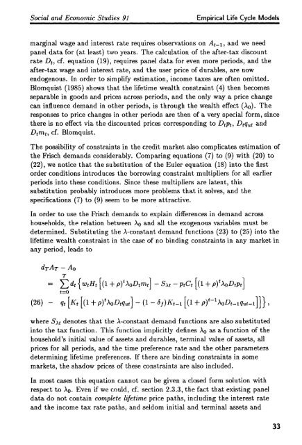
dTAT - Ao<br />
Edt {wtHt [(I.+ p) . tÀ0Dont] - St - PtC t [(1- AoDtPt]<br />
t=o<br />
(26) - qt[Kt[(1 + Aoptqut] - (1 - (5f)Kt-1[(1+ P) t_ l Aopt-iqut-1]1}<br />
where S At denotes that the A-constant dem<strong>and</strong> functions are also substituted<br />
into the tax function. This function implicitly defines )to as a function <strong>of</strong> the<br />
household's initial value <strong>of</strong> assets <strong>and</strong> durables, terminal value <strong>of</strong> assets, all<br />
prices for all periods, <strong>and</strong> the time preference rate <strong>and</strong> the other parameters<br />
determining <strong>life</strong>time preferences. If there are binding constraints in some<br />
markets, the shadow prices <strong>of</strong> these constraints are also included.<br />
In most cases this equation cannot can be given a closed form solution with<br />
respect to Ao. Even if we could, cf. section 2.3.3, the fact that existing panel<br />
data do not contain complete <strong>life</strong>time price paths, including the interest rate<br />
<strong>and</strong> the income tax rate paths, <strong>and</strong> seldom initial <strong>and</strong> terminal assets <strong>and</strong><br />
33


