Empirical life cycle models of labour supply and - Statistisk sentralbyrå
Empirical life cycle models of labour supply and - Statistisk sentralbyrå
Empirical life cycle models of labour supply and - Statistisk sentralbyrå
You also want an ePaper? Increase the reach of your titles
YUMPU automatically turns print PDFs into web optimized ePapers that Google loves.
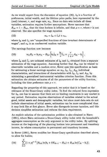
Social <strong>and</strong> Economic Studies 91 <strong>Empirical</strong> Life Cycle Models<br />
As we would expect from the discussion <strong>of</strong> equation (26), Ao is a function <strong>of</strong><br />
preferences, initial wealth, <strong>and</strong> the <strong>life</strong>time price paths, here represented by the<br />
(real) interest, r, <strong>and</strong> wage rate, wit . Since no data sets include all these<br />
variables, estimation requires further assumptions. Boyer assumes that<br />
Bcit = 1 — Bhit, that the time horizon is infinite, <strong>and</strong> that p = r, where r is not<br />
observed. She also specifies the wage equation<br />
(52) wit = 10i -F /lit -F<br />
where ioi <strong>and</strong> /ii are "unspecified functions <strong>of</strong> time invariant determinants <strong>of</strong><br />
wages", <strong>and</strong> vit is an unobserved r<strong>and</strong>om variable.<br />
The earnings function now becomes<br />
bh r<br />
(53)<br />
witHit = bhwit Bhit[bhi0i + 1 + r itio — b]<br />
where ioi <strong>and</strong> 1i1 are unbiased estimates <strong>of</strong> toi <strong>and</strong> hi obtained from a separate<br />
estimation <strong>of</strong> the wage equation. Assuming further that Bhit can be related to<br />
observable variables <strong>and</strong> a r<strong>and</strong>om error, Boyer uses this specification as basis<br />
for estimating a linear earnings equation on wit , ioi , 11 , A 0 , individual<br />
characteristics, <strong>and</strong> interactions <strong>of</strong> characteristics with ioi, Iii <strong>and</strong> Aio, by<br />
minimizing a generalized instrumental variables criterion function. From this<br />
estimation she obtains estimates <strong>of</strong> all the parameters <strong>of</strong> the utility function,<br />
including the time preference rate p = r.<br />
Regarding the properties <strong>of</strong> this approach, we notice that it is based on the<br />
relevance <strong>of</strong> the Stone-Geary utility index. To find the reduced form expression<br />
for Ao , one has to assume that there are no binding constraints in any market in<br />
any period. Estimation requires observations <strong>of</strong> variables related to the actual<br />
good, initial assets <strong>and</strong> demographic variables, but since most data sets do not<br />
include observations <strong>of</strong> initial assets, estimation can be more complicated than<br />
it may look like at first glance. Boyer also disregards income taxation, <strong>and</strong> this<br />
decision simplifies estimation <strong>and</strong> reduces the data requirement.<br />
An explicit solution <strong>of</strong> the optimization problem is also obtained in Biørn<br />
(1981), where Biørn estimates a Stone-Geary utility index with the household's<br />
aggregate consumption as the only argument in the utility index. By splitting<br />
income at the beginning <strong>of</strong> the planning horizon into permanent <strong>and</strong> transitory<br />
income, he relates consumption to permanent <strong>and</strong> transitory incomes.<br />
In Bover (1991), Boyer modifies her Stone-Geary specification described above,<br />
to allow for habits;<br />
(54) E(1 + p)tk [Bhikin(bh+ Hik) Bk in (Cik — bc)} •<br />
k=t<br />
43


