economia de energia e redução do pico da curva de demanda para ...

30
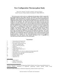
Fig. 3.1 Diagrama mostrando um circuito termossifão e a distribuição hipotética de
temperatura
2
1 ⎡
( h ⎤
3
− h5
)
h T
= ( S1
− S
2
) ⋅ ⎢2(
h3
− h2
) − ( h2
− h1
) − ⎥
(3.1)
2 ⎣
h6
− h5
⎦
onde
h
T
é o ganho-termossifão, h x
são diferentes alturas do sistema (Fig. 3.1) e S é uma
aproximação parabólica da densidade específica da água dada por,
2
S = AT + BT + C
(3.2)
Na Eq. 3.2,
−6
A = −4,05⋅10
[°C -2 ];
−5
B = −3,906
⋅10
[°C -1 ]; = 1, 00026
C [-] (3.3)
Definindo,
g(
h)
( h
− h )
2
3 5
= 2( h3
− h2
) − ( h2
− h1
) −
(3.4)
h6
− h5