2. Grundlagen der Booleschen Algebra - Fachgebiet Rechnersysteme
2. Grundlagen der Booleschen Algebra - Fachgebiet Rechnersysteme
2. Grundlagen der Booleschen Algebra - Fachgebiet Rechnersysteme

Erfolgreiche ePaper selbst erstellen
Machen Sie aus Ihren PDF Publikationen ein blätterbares Flipbook mit unserer einzigartigen Google optimierten e-Paper Software.
<strong>Fachgebiet</strong> <strong>Rechnersysteme</strong>1<br />
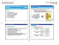
<strong>2.</strong> <strong>Grundlagen</strong> <strong>der</strong> <strong>Booleschen</strong> <strong>Algebra</strong><br />
Inhalt<br />
<strong>2.</strong>1 Boolesche Elementaroperationen<br />
<strong>2.</strong>2 Boolesche Funktionen, Funktionstabellen<br />
<strong>2.</strong>3 Boolesche Terme<br />
<strong>2.</strong>4 Elementare Gleichungen <strong>der</strong> booleschen <strong>Algebra</strong><br />
<strong>2.</strong>5 Veitch-Diagramme<br />
<strong>2.</strong>6 Produkt- und Summenterme<br />
<strong>2.</strong>7 Disjunktive und konjunktive Normalformen<br />
<strong>2.</strong>8 Vollständige Verknüpfungssysteme<br />
<strong>2.</strong>9 Der Entwicklungssatz von Boole<br />
<strong>2.</strong>10 Gattergleichungen und Gatternetze<br />
Vorlesung Logischer Entwurf
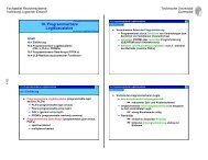
Lernziele von Kap. 2:<br />
� Bedeutung <strong>der</strong> booleschen Grundverknüpfungen kennen<br />
(Und, O<strong>der</strong>, Nicht, Nand, Nor, Exor)<br />
� Gesetze <strong>der</strong> booleschen <strong>Algebra</strong> kennen und effizient<br />
anwenden (Terme vereinfachen)<br />
� Veitch-Diagramm �� boolescher Term<br />
� Konzepte: Produkt- und Summenterme, Minterm, Maxterm,<br />
De Morgan'scher Satz, DNF, KNF, Reed-Muller-Form,<br />
Nand/Nand- und Nor/Nor-Realisierungen, Boolescher<br />
Entwicklungssatz, Multiplexor kennen<br />
� boolescher Term �� Gatternetz<br />
2
<strong>2.</strong>1 Boolesche Elementaroperationen<br />
� Und-Verknüpfung (Konjunktion)<br />
a b a⋅b 0 0 0<br />
0 1 0<br />
1 0 0<br />
1 1 1<br />
� 0-Dominanz<br />
a<br />
b<br />
a<br />
b<br />
a<br />
b<br />
Gattersymbole<br />
&<br />
DIN (alt)<br />
IEEE-<br />
Standard<br />
3<br />
US-Norm<br />
(alt)
<strong>2.</strong>1 Boolesche Elementaroperationen<br />
— Anwendungsbeispiele:<br />
� ist a = 1, folgt <strong>der</strong> Ausgang dem Eingang b<br />
� ist a = 0, ist <strong>der</strong> Ausgang = 0 unabhängig<br />
von b<br />
a b a⋅b 0 0 0<br />
0 1 0<br />
1 0 0<br />
1 1 1<br />
a<br />
b<br />
� ein Und-Gatter kann als steuerbares Tor<br />
benutzt werden<br />
&<br />
4
<strong>2.</strong>1 Boolesche Elementaroperationen<br />
� O<strong>der</strong>-Verknüpfung (Disjunktion)<br />
a b a+ b<br />
0 0 0<br />
0 1 1<br />
1 0 1<br />
1 1 1<br />
� 1-Dominanz<br />
a<br />
b<br />
a<br />
b<br />
a<br />
b<br />
Gattersymbole<br />
≥1<br />
DIN (alt)<br />
IEEE-<br />
Standard<br />
US-Norm<br />
(alt)<br />
5
<strong>2.</strong>1 Boolesche Elementaroperationen<br />
� Negation Gattersymbole<br />
a a<br />
0 1<br />
1 0<br />
a DIN (alt)<br />
a 1<br />
IEEE-<br />
Standard<br />
a US-Norm<br />
(alt)<br />
6
<strong>2.</strong>1 Boolesche Elementaroperationen<br />
� bei Gattern ist <strong>der</strong> Informationsfluß<br />
gerichtet, es wird zwischen Ein- und<br />
Ausgängen unterschieden (im Gegensatz<br />
beispielsweise zu einem ohmschen<br />
Wi<strong>der</strong>stand)<br />
7
<strong>2.</strong>1 Boolesche Elementaroperationen<br />
� Weitere Notationen sind gebräuchlich, z.B.<br />
a • b a ∧ b a & b<br />
a + b a ∨ b a | b<br />
a ¬a a'<br />
aussagenlogische Symbole<br />
8
<strong>2.</strong>2 <strong>2.</strong>2 Boolesche Funktionen, Funktionstabellen<br />
Funktionstabellen<br />
� In vielen Fällen ist es bei dem Entwurf eines Systems<br />
sinnvoll, mit Tabellen zu arbeiten<br />
— sehr einfaches Beispiel:<br />
gesucht ist eine Schaltung zur Prüfung einer Ampel.<br />
die Schaltung soll genau dann den Wert 1 liefern,<br />
wenn die Ampel eine zulässige Kombination von<br />
Lichtern anzeigt (z.B. nur grün).<br />
eine 0 soll bei einer unzulässigen Kombination<br />
angezeigt werden.<br />
9
<strong>2.</strong>2 Boolesche Funktionen, Funktionstabellen<br />
— Eingänge: r rot, g grün, e gelb<br />
r = 0: rotes Licht aus, r = 1: rotes Licht an, usw.<br />
— Ausgang: p<br />
— drei Eingänge, die jeweils zwei Werte annehmen<br />
können: systematisch gibt es offenbar 2 3 =8<br />
Fälle (Eingangskombinationen), die untersucht<br />
werden müssen<br />
� die folgende Darstellung in Tabellenform<br />
hilft, alle Fälle zu berücksichtigen<br />
r<br />
e<br />
g<br />
Ampelprüfer<br />
p<br />
10
<strong>2.</strong>2 Boolesche Funktionen, Funktionstabellen<br />
— Eingänge: r rot, g grün, e gelb<br />
2 3 = 8 Fälle<br />
r<br />
e<br />
g<br />
r e g p?<br />
0 0 0<br />
0 0 1<br />
0 1 0<br />
0 1 1<br />
1 0 0<br />
1 0 1<br />
1 1 0<br />
1 1 1<br />
Ampelprüfer<br />
p<br />
11
<strong>2.</strong>2 Boolesche Funktionen, Funktionstabellen<br />
� Im Beispiel sind r, e, g und p boolesche Variable<br />
� Eine boolesche Variable kann einen <strong>der</strong> Werte 0 o<strong>der</strong> 1 aus<br />
<strong>der</strong> booleschen Wertemenge B = {0, 1} annehmen<br />
� Allgemein ist eine boolesche Funktion F von n Variablen<br />
eine Funktion<br />
F: B n → B<br />
� eine solche Funktion modelliert eine<br />
Schaltung mit n Eingängen und einem<br />
Ausgang, im Beispiel also B 3 → B<br />
r<br />
e<br />
g<br />
Ampelprüfer<br />
p<br />
12
<strong>2.</strong>2 Boolesche Funktionen, Funktionstabellen<br />
� Durch eine Boolesche Funktion F in n Variablen wird<br />
je<strong>der</strong> <strong>der</strong> 2 n Wertekombinationen <strong>der</strong> Eingangsvariablen<br />
ein eindeutiger Wert zugeordnet (Funktionsbegriff)<br />
F: B n → B<br />
� dies entspricht erwünschtem deterministischem<br />
Systemverhalten<br />
r<br />
e<br />
g<br />
Ampelprüfer<br />
p<br />
13
<strong>2.</strong>2 Boolesche Funktionen, Funktionstabellen<br />
� Unter einem Funktionsbündel versteht man eine Funktion<br />
F: B n → B m<br />
� ein Funktionsbündel modelliert eine<br />
Schaltung mit mehreren Ausgängen, im<br />
Beispiel unten etwa B 3 → B 2<br />
r<br />
e<br />
g<br />
an<strong>der</strong>e<br />
Schaltung<br />
p<br />
q<br />
14
<strong>2.</strong>2 Boolesche Funktionen, Funktionstabellen<br />
� Hier ein Beispiel einer Funktionstabelle<br />
mit vier booleschen<br />
Variablen x 1 , x 2 , x 3 , x 4<br />
� Wir schreiben<br />
f(x 1 , x 2 , x 3 , x 4 )<br />
und zum Beispiel<br />
f(0,1,0,1) = 1<br />
� die Funktionstabelle<br />
<strong>der</strong> Funktion in vier<br />
Variablen hat 2 4<br />
Zeilen<br />
x 1 x 2 x 3<br />
x 4<br />
f<br />
0 0 0 0 0<br />
0 0 0 1 1<br />
0 0 1 0 0<br />
0 0 1 1 0<br />
0 1 0 0 1<br />
0 1 0 1 1<br />
0 1 1 0 0<br />
0 1 1 1 1<br />
1 0 0 0 0<br />
1 0 0 1 1<br />
1 0 1 0 0<br />
1 0 1 1 0<br />
1 1 0 0 1<br />
1 1 0 1 1<br />
1 1 1 0 0<br />
1 1 1 1 1<br />
15
<strong>2.</strong>2 Boolesche Funktionen, Funktionstabellen<br />
Problem: die Größe von Funktionstabellen wächst<br />
exponentiell mit <strong>der</strong> Anzahl <strong>der</strong> Variablen<br />
16
<strong>2.</strong>2 Boolesche Funktionen, Funktionstabellen<br />
� Die Dezimaläquivalent-Darstellung einer<br />
booleschen Funktion<br />
� Zuordnung von Dezimaläquivalenten<br />
zu Wertekombinationen <strong>der</strong><br />
Variablen entsprechend einer<br />
Wertigkeit<br />
� Repräsentation durch die Menge<br />
aller Wertekombinationen für f = 1<br />
f = {1,4,5,7,9,12,13,15}<br />
0<br />
1<br />
2<br />
3<br />
4<br />
5<br />
6<br />
7<br />
8<br />
9<br />
10<br />
11<br />
12<br />
13<br />
14<br />
15<br />
2222<br />
xxxx<br />
3 2 1 0<br />
3 2 1 0<br />
f<br />
0 0 0 0 0<br />
0 0 0 1 1<br />
0 0 1 0 0<br />
0 0 1 1 0<br />
0 1 0 0 1<br />
0 1 0 1 1<br />
0 1 1 0 0<br />
0 1 1 1 1<br />
1 0 0 0 0<br />
1 0 0 1 1<br />
1 0 1 0 0<br />
1 0 1 1 0<br />
1 1 0 0 1<br />
1 1 0 1 1<br />
1 1 1 0 0<br />
1 1 1 1 1<br />
17
<strong>2.</strong>3 <strong>2.</strong>4 Boolesche Terme<br />
� Boolesche Terme sind textliche Darstellungen von<br />
booleschen Funktionen, z.B.<br />
� Die Syntax boolescher Terme:<br />
� die Konstanten 0 und 1 sind boolesche Terme<br />
� Literale, d.h. Variablen o<strong>der</strong> ihre Negation sind<br />
boolesche Terme, z.B. a und a<br />
� sind a und b boolesche Terme, dann sind auch<br />
(a ⋅ b),<br />
boolesche Terme<br />
a ⋅ b ⋅ c + c ⋅a<br />
⋅ (e<br />
(a<br />
+ b),<br />
+ b)<br />
a<br />
18
<strong>2.</strong>3 Boolesche Terme<br />
� Klammern sind notwendig, um die Eindeutigkeit zu sichern,<br />
— Beispiel: a • b + c,<br />
bedeutet dies (a • b) + c o<strong>der</strong> a • (b + c) ?<br />
� Klammern können dadurch wegfallen, daß die Eindeutigkeit<br />
durch die Zuordnung von Prioritäten ("Punkt vor Strich")<br />
gesichert wird:<br />
Und (•) bindet stärker als O<strong>der</strong> (+),<br />
d.h. a • b + c bedeutet (a • b) + c<br />
� Weiterhin kann das Symbol für die Und-Verknüpfung<br />
weggelassen werden, falls eine entsprechende Vereinbarung<br />
über die Variablennamen getroffen wird<br />
— Beispiel: nur ein Buchstabe ist als Variablenname<br />
erlaubt � ab + c ist eindeutig a•b + c<br />
� Die beiden äußersten Klammern können (selbstverständlich)<br />
weggelassen werden<br />
19
<strong>2.</strong>3 Boolesche Terme<br />
� Die Beziehung zwischen<br />
booleschen Termen und<br />
booleschen Funktionen<br />
� die Konstanten bezeichnen<br />
konstante Funktionen,<br />
Beispiel: 0<br />
0<br />
1<br />
2<br />
3<br />
4<br />
5<br />
6<br />
7<br />
8<br />
9<br />
10<br />
11<br />
12<br />
13<br />
14<br />
15<br />
2222<br />
xxxx<br />
3 2 1 0<br />
3 2 1 0 0<br />
0 0 0 0 0<br />
0 0 0 1 0<br />
0 0 1 0 0<br />
0 0 1 1 0<br />
0 1 0 0 0<br />
0 1 0 1 0<br />
0 1 1 0 0<br />
0 1 1 1 0<br />
1 0 0 0 0<br />
1 0 0 1 0<br />
1 0 1 0 0<br />
1 0 1 1 0<br />
1 1 0 0 0<br />
1 1 0 1 0<br />
1 1 1 0 0<br />
1 1 1 1 0<br />
20
<strong>2.</strong>3 Boolesche Terme<br />
� Die Literale bezeichnen<br />
Funktionen, die genau für<br />
diejenigen Werte gleich 1 sind,<br />
für die die Variable gleich 1<br />
bzw. gleich 0 ist<br />
0<br />
1<br />
2<br />
3<br />
4<br />
5<br />
6<br />
7<br />
8<br />
9<br />
10<br />
11<br />
12<br />
13<br />
14<br />
15<br />
2222<br />
xxxx<br />
3 2 1 0<br />
3 2 1 0<br />
x x<br />
2 2<br />
0 0 0 0 0 1<br />
0 0 0 1 0 1<br />
0 0 1 0 0 1<br />
0 0 1 1 0 1<br />
0 1 0 0 1 0<br />
0 1 0 1 1 0<br />
0 1 1 0 1 0<br />
0 1 1 1 1 0<br />
1 0 0 0 0 1<br />
1 0 0 1 0 1<br />
1 0 1 0 0 1<br />
1 0 1 1 0 1<br />
1 1 0 0 1 0<br />
1 1 0 1 1 0<br />
1 1 1 0 1 0<br />
1 1 1 1 1 0<br />
21
<strong>2.</strong>3 Boolesche Terme<br />
� Die Bedeutung weiterer<br />
Verknüpfungen ergibt sich für<br />
0<br />
jede Wertekombination durch<br />
1<br />
Anwendung <strong>der</strong> Definition <strong>der</strong> 2<br />
Verknüpfungen<br />
3<br />
4<br />
5<br />
6<br />
7<br />
8<br />
9<br />
10<br />
11<br />
12<br />
13<br />
14<br />
15<br />
2222<br />
xxxx<br />
3 2 1 0<br />
3 2 1 0<br />
x2 x3 x2 ⋅ x3<br />
0 0 0 0 0 1 0<br />
0 0 0 1 0 1 0<br />
0 0 1 0 0 1 0<br />
0 0 1 1 0 1 0<br />
0 1 0 0 1 1 1<br />
0 1 0 1 1 1 1<br />
0 1 1 0 1 1 1<br />
0 1 1 1 1 1 1<br />
1 0 0 0 0 0 0<br />
1 0 0 1 0 0 0<br />
1 0 1 0 0 0 0<br />
1 0 1 1 0 0 0<br />
1 1 0 0 1 0 0<br />
1 1 0 1 1 0 0<br />
1 1 1 0 1 0 0<br />
1 1 1 1 1 0 0<br />
22
<strong>2.</strong>3 Boolesche Terme<br />
� Eine an<strong>der</strong>e Möglichkeit, die boolesche Funktion aus<br />
einem Term zu ermitteln, ist es, alle Wertekombinationen<br />
<strong>der</strong> Variablen in den Term einzusetzen und jeweils den<br />
Funktionswert zu bestimmen (den Term für die<br />
Wertekombination auszuwerten).<br />
— Beispiel: es sei f(a,b,c,d) = a + b + cd.<br />
Für a=0, b=0, c=0, d=1 ergibt sich entsprechend<br />
den Funktionstabellen für die Und- und O<strong>der</strong>-<br />
Verknüpfung <strong>der</strong> Wert f(0,0,0,1) = 0, usw.<br />
23
<strong>2.</strong>4 Elementare Gleichungen <strong>der</strong> booleschen <strong>Algebra</strong><br />
� Zwei boolesche Terme f und g sind gleich, f = g, wenn<br />
für alle Wertekombinationen <strong>der</strong> Variablen eine<br />
Auswertung <strong>der</strong> Terme denselben Wert ergibt<br />
� In <strong>der</strong> booleschen <strong>Algebra</strong> gelten die folgenden<br />
Gleichungen:<br />
(T1) x + 0 = x (T1') x • 1 = x Identität<br />
(T2) x + 1 = 1 (T2') x • 0 = 0 Eins/Null-Element<br />
(T3) x + x = x (T3') x • x = x Idempotenz<br />
(T4) x = x (T4') 1 = 0 Involution<br />
(T5) x + x = 1 (T5') x • x = 0 Komplement<br />
24
<strong>2.</strong>4 Elementare Gleichungen <strong>der</strong> booleschen <strong>Algebra</strong><br />
(T6) x + y = y + x (T6') x • y = y • x Kommutativität<br />
(T7) (x + y) + z = x + (y + z) = x + y + z Assoziativität<br />
(T7') (x • y) • z = x • (y • z) = x • y • z<br />
(T8) x•y + x•z = x•(y + z) Distributivität<br />
(T8') (x + y)•(x + z) = x + y•z<br />
(T9) (x + y) = x • y (T9') (x • y) = x + y De Morgan'scher<br />
Satz<br />
(T10) (x 1 +...+ x n )= x 1 •...• x n<br />
(T10') (x 1 •...• x n )= x 1 +...+ x n<br />
generalisierter<br />
De Morgan'scher<br />
Satz<br />
25
<strong>2.</strong>4 Elementare Gleichungen <strong>der</strong> booleschen <strong>Algebra</strong><br />
(T11) x + x•y = x + y (T11') x•(x + y) = x•y<br />
(T12) x + x•y = x (T12') x•(x + y) = x<br />
x<br />
x<br />
y<br />
&<br />
Absorption<br />
� grundlegende Bedeutung für die Vereinfachung<br />
von Schaltungen und Termen, z.B.<br />
≥1<br />
x<br />
y<br />
≥1<br />
26
<strong>2.</strong>4 Elementare Gleichungen <strong>der</strong> booleschen <strong>Algebra</strong><br />
(T13) x•y + x•z + y•z = x•y + x•z<br />
(T13') (x + y)•(x + z)•(y + z) = (x + y)•(x + z)<br />
Konsensus<br />
� es gibt offenbar für dieselbe Funktion viele<br />
Termdarstellungen<br />
27
<strong>2.</strong>4 Elementare Gleichungen <strong>der</strong> booleschen <strong>Algebra</strong><br />
� Weitere Vereinfachungstechnik für Terme (Kombination<br />
T8, T5, T1):<br />
x<br />
y<br />
x<br />
y<br />
x⋅ y+ x⋅ y = x ⋅ (y+ y) = x⋅ 1= x<br />
(x + y) ⋅ (x + y) = x + y ⋅ y = x + 0 = x<br />
&<br />
&<br />
≥1<br />
x<br />
28
<strong>2.</strong>4 Elementare Gleichungen <strong>der</strong> booleschen <strong>Algebra</strong><br />
� Noch eine Vereinfachungstechnik für Terme (Erweitern<br />
T1, T5, T8 und Absorption T12): Beispiel T13<br />
x<br />
x<br />
⋅<br />
⋅<br />
y<br />
y<br />
+<br />
+<br />
x<br />
x<br />
⋅ z +<br />
⋅ z<br />
y<br />
⋅<br />
z<br />
=<br />
x<br />
⋅<br />
y<br />
+<br />
x<br />
⋅<br />
z<br />
+<br />
x<br />
⋅<br />
y<br />
⋅<br />
z<br />
+<br />
x<br />
⋅<br />
y<br />
⋅<br />
z<br />
=<br />
29
<strong>2.</strong>4 Elementare Gleichungen <strong>der</strong> booleschen <strong>Algebra</strong><br />
� Das algebraische System<br />
(B, +, ⋅ , 0, 1)<br />
das die Eigenschaften T1, T5, T6, T8 (Identität,<br />
Komplement, Kommutativität, Distributivität) besitzt, ist<br />
eine boolesche <strong>Algebra</strong> (Boole 1854).<br />
(Anm.: die Negation wird nicht als Operator, son<strong>der</strong>n als<br />
Bezeichner des inversen Elements angesehen,<br />
Huntington'schen Axiome)<br />
� Beispiel einer an<strong>der</strong>en booleschen <strong>Algebra</strong> (S ist eine<br />
beliebige Menge):<br />
S<br />
(2 , ∪, ∩, ∅,<br />
S)<br />
30
<strong>2.</strong>4 Elementare Gleichungen <strong>der</strong> booleschen <strong>Algebra</strong><br />
� Nachtrag einiger weiterer boolescher Elementaroperationen:<br />
� Exor ⊕ (Exklusiv-O<strong>der</strong>, Ungleich, Addition modulo 2)<br />
Definition: a ⊕ b = a ⋅ b + a ⋅b<br />
a b a ⊕b<br />
0<br />
0<br />
1<br />
1<br />
0<br />
1<br />
0<br />
1<br />
0<br />
1<br />
1<br />
0<br />
a<br />
b<br />
a<br />
b<br />
a<br />
b<br />
Gattersymbole<br />
⊕<br />
=1<br />
DIN (alt)<br />
31<br />
IEEE-<br />
Standard<br />
US-Norm<br />
(alt)
<strong>2.</strong>4 Elementare Gleichungen <strong>der</strong> booleschen <strong>Algebra</strong><br />
— die Exor-Verknüpfung ist kommutativ und<br />
assoziativ, d.h. es gilt z.B.<br />
a ⊕ b ⊕ c = c ⊕ b ⊕ a<br />
— weitere Eigenschaften:<br />
x ⊕ x = 0,<br />
x ⊕ 0 = x,<br />
x ⊕ 1 = ⌧<br />
32
<strong>2.</strong>4 Elementare Gleichungen <strong>der</strong> booleschen <strong>Algebra</strong><br />
� NAND<br />
a b (a⋅b)<br />
0<br />
0<br />
1<br />
1<br />
0<br />
1<br />
0<br />
1<br />
1<br />
1<br />
1<br />
0<br />
a<br />
b<br />
a<br />
b<br />
a<br />
b<br />
Gattersymbole<br />
&<br />
DIN (alt)<br />
IEEE-<br />
Standard<br />
US-Norm<br />
(alt)<br />
33
<strong>2.</strong>4 Elementare Gleichungen <strong>der</strong> booleschen <strong>Algebra</strong><br />
� NOR<br />
a b (a+<br />
b)<br />
0<br />
0<br />
1<br />
1<br />
0<br />
1<br />
0<br />
1<br />
1<br />
0<br />
0<br />
0<br />
a<br />
b<br />
a<br />
b<br />
a<br />
b<br />
Gattersymbole<br />
≥1<br />
DIN (alt)<br />
IEEE-<br />
Standard<br />
US-Norm<br />
(alt)<br />
34
<strong>2.</strong>4 Elementare Gleichungen <strong>der</strong> booleschen <strong>Algebra</strong><br />
� Die Implikation →:<br />
a<br />
� Die Äquivalenz ≡ (Gleichheit):<br />
a<br />
→<br />
≡<br />
b<br />
b<br />
=<br />
a + b<br />
= a ⋅b<br />
+ a ⋅ b<br />
— die Äquivalenz ist genau dann gleich 1, wenn die<br />
Argumente den gleichen Wert haben<br />
— die Exor-Funktion ist genau dann gleich 1, wenn<br />
die Argumente ungleichen Wert haben<br />
— es gilt: a ≡ b = (a ⊕ b)<br />
35
<strong>2.</strong>4 Elementare Gleichungen <strong>der</strong> booleschen <strong>Algebra</strong><br />
� Technisch gibt es Und-, O<strong>der</strong>-, Nand-, Nor-, ... -Gatter<br />
mit mehr als zwei (typisch: maximal 8) Eingängen<br />
— Beispiele:<br />
&<br />
&<br />
� wegen <strong>der</strong> Kommutativität und Assoziativität<br />
<strong>der</strong> Und- und O<strong>der</strong>-Operation (T6/T7) spielt die<br />
Reihenfolge <strong>der</strong> Eingänge keine Rolle<br />
≥1<br />
& &<br />
36
<strong>2.</strong>5 Veitch-Diagramme<br />
� Veitch-Diagramme sind ein wichtiges Hilfsmittel für den<br />
manuellen Entwurf von Schaltungen für Probleme mit bis<br />
zu sechs Variablen<br />
� Veitch-Diagramme stellen boolesche Funktionen in<br />
Matrixform dar<br />
37
<strong>2.</strong>5 Veitch-Diagramme<br />
�<br />
0<br />
1<br />
2<br />
3<br />
4<br />
5<br />
6<br />
7<br />
8<br />
9<br />
10<br />
11<br />
12<br />
13<br />
14<br />
15<br />
2222<br />
xxxx<br />
3 2 1 0<br />
3 2 1 0 f<br />
0 0 0 0 0<br />
0 0 0 1 1<br />
0 0 1 0 0<br />
0 0 1 1 0<br />
0 1 0 0 1<br />
0 1 0 1 1<br />
0 1 1 0 0<br />
0 1 1 1 1<br />
1 0 0 0 0<br />
1 0 0 1 1<br />
1 0 1 0 0<br />
1 0 1 1 0<br />
1 1 0 0 1<br />
1 1 0 1 1<br />
1 1 1 0 0<br />
1 1 1 1 1<br />
Beispiel: Veitch-Diagramm<br />
in vier Variablen<br />
x 0<br />
0<br />
1<br />
3<br />
2<br />
4<br />
5<br />
7<br />
6<br />
�<br />
x 2<br />
12<br />
x 3<br />
13<br />
15<br />
14<br />
38<br />
markiert alle<br />
Fel<strong>der</strong> mit x 3 = 1<br />
8<br />
9<br />
11<br />
10<br />
x 1
<strong>2.</strong>5 Veitch-Diagramme<br />
0<br />
1<br />
2<br />
3<br />
4<br />
5<br />
6<br />
7<br />
8<br />
9<br />
10<br />
11<br />
12<br />
13<br />
14<br />
15<br />
2222<br />
xxxx<br />
3 2 1 0<br />
3 2 1 0 f<br />
0 0 0 0 0<br />
0 0 0 1 1<br />
0 0 1 0 0<br />
0 0 1 1 0<br />
0 1 0 0 1<br />
0 1 0 1 1<br />
0 1 1 0 0<br />
0 1 1 1 1<br />
1 0 0 0 0<br />
1 0 0 1 1<br />
1 0 1 0 0<br />
1 0 1 1 0<br />
1 1 0 0 1<br />
1 1 0 1 1<br />
1 1 1 0 0<br />
1 1 1 1 1<br />
x 0<br />
0<br />
1<br />
3<br />
2<br />
4<br />
5<br />
7<br />
6<br />
x 2<br />
12<br />
13<br />
15<br />
14<br />
x 3<br />
8<br />
9<br />
11<br />
10<br />
x 1<br />
39
<strong>2.</strong>5 Veitch-Diagramme<br />
0<br />
1<br />
2<br />
3<br />
4<br />
5<br />
6<br />
7<br />
8<br />
9<br />
10<br />
11<br />
12<br />
13<br />
14<br />
15<br />
2222<br />
xxxx<br />
3 2 1 0<br />
3 2 1 0 f<br />
0 0 0 0 0<br />
0 0 0 1 1<br />
0 0 1 0 0<br />
0 0 1 1 0<br />
0 1 0 0 1<br />
0 1 0 1 1<br />
0 1 1 0 0<br />
0 1 1 1 1<br />
1 0 0 0 0<br />
1 0 0 1 1<br />
1 0 1 0 0<br />
1 0 1 1 0<br />
1 1 0 0 1<br />
1 1 0 1 1<br />
1 1 1 0 0<br />
1 1 1 1 1<br />
Eintragen <strong>der</strong> Funktionswerte:<br />
x 0<br />
0 1 1 0<br />
1<br />
0<br />
0<br />
0<br />
1<br />
3<br />
2<br />
1<br />
1<br />
0<br />
4<br />
5<br />
7<br />
6<br />
x 2<br />
1<br />
1<br />
0<br />
12<br />
13<br />
15<br />
14<br />
x 3<br />
1<br />
0<br />
0<br />
8<br />
9<br />
11<br />
10<br />
x 1<br />
40
<strong>2.</strong>5 Veitch-Diagramme<br />
� Von zentraler Bedeutung sind die Nachbarschaftsbeziehungen<br />
in Veitch-Diagrammen: zwei benachbarte<br />
Fel<strong>der</strong> unterscheiden sich nämlich in genau einer<br />
Variablen<br />
41
<strong>2.</strong>5 Veitch-Diagramme<br />
hier<br />
än<strong>der</strong>n<br />
sich vier<br />
Variable<br />
0<br />
1<br />
2<br />
3<br />
4<br />
5<br />
6<br />
7<br />
8<br />
9<br />
10<br />
11<br />
12<br />
13<br />
14<br />
15<br />
2222<br />
xxxx<br />
3 2 1 0<br />
3 2 1 0 f<br />
0 0 0 0 0<br />
0 0 0 1 1<br />
0 0 1 0 0<br />
0 0 1 1 0<br />
0 1 0 0 1<br />
0 1 0 1 1<br />
0 1 1 0 0<br />
0 1 1 1 1<br />
1 0 0 0 0<br />
1 0 0 1 1<br />
1 0 1 0 0<br />
1 0 1 1 0<br />
1 1 0 0 1<br />
1 1 0 1 1<br />
1 1 1 0 0<br />
1 1 1 1 1<br />
hier än<strong>der</strong>t sich jeweils<br />
nur eine Variable<br />
x 0<br />
0<br />
1<br />
0<br />
0<br />
0<br />
1<br />
3<br />
2<br />
1<br />
1<br />
1<br />
0<br />
4<br />
5<br />
7<br />
6<br />
x 2<br />
1<br />
1<br />
1<br />
0<br />
12<br />
13<br />
15<br />
14<br />
x 3<br />
0<br />
1<br />
0<br />
0<br />
8<br />
9<br />
11<br />
10<br />
x 1<br />
42
<strong>2.</strong>5 Veitch-Diagramme<br />
dies gilt auch bei den<br />
Randfel<strong>der</strong>n (a)<br />
x 0<br />
0<br />
1<br />
0<br />
0<br />
0<br />
1<br />
3<br />
2<br />
1<br />
1<br />
1<br />
0<br />
4<br />
5<br />
7<br />
6<br />
x 2<br />
1<br />
1<br />
1<br />
0<br />
12<br />
13<br />
15<br />
14<br />
x 3<br />
0<br />
1<br />
0<br />
8<br />
9<br />
11<br />
010 10<br />
x 1<br />
43
<strong>2.</strong>5 Veitch-Diagramme<br />
das gilt auch bei den<br />
Randfel<strong>der</strong>n (b)<br />
x 0<br />
0<br />
1<br />
0<br />
0<br />
0<br />
1<br />
3<br />
2<br />
1<br />
1<br />
1<br />
0<br />
4<br />
5<br />
7<br />
6<br />
x 2<br />
1<br />
1<br />
1<br />
0<br />
12<br />
13<br />
15<br />
14<br />
x 3<br />
0<br />
1<br />
0<br />
0<br />
8<br />
9<br />
11<br />
10<br />
x 1<br />
44
<strong>2.</strong>5 Veitch-Diagramme<br />
x 0<br />
Veitch-Diagramme in zwei und drei Variablen<br />
0 2<br />
1<br />
x 1<br />
3<br />
x 0<br />
0 2<br />
1<br />
6<br />
x 2<br />
4<br />
3 7 5<br />
x 1<br />
45
<strong>2.</strong>5 Veitch-Diagramme<br />
x 0<br />
Veitch-Diagramm in fünf Variablen<br />
0<br />
1<br />
3<br />
2<br />
4<br />
5<br />
7<br />
6<br />
x 2<br />
12<br />
13<br />
15<br />
14<br />
8<br />
9<br />
11<br />
10<br />
x 3<br />
24<br />
25<br />
27<br />
26<br />
28<br />
29<br />
31<br />
30<br />
x 2<br />
x 4<br />
20<br />
21<br />
23<br />
22<br />
16<br />
17<br />
19<br />
18<br />
x 1<br />
46
<strong>2.</strong>5 Veitch-Diagramme<br />
Problem: <strong>der</strong> Darstellungsaufwand (Platz) wächst auch<br />
bei Veitch-Diagrammen exponentiell in <strong>der</strong> Anzahl <strong>der</strong><br />
Variablen<br />
— Beispiel: 32-bit Addierer ~ 264 Fel<strong>der</strong> !<br />
� Veitch-Diagramme sind sinnvoll bis zu 6<br />
Variablen<br />
� Alternativen u.a.:<br />
� textliche Darstellungen (Abschnitt <strong>2.</strong>4)<br />
� sog. Entscheidungsgraphen (Abschnitt 3.2)<br />
47
<strong>2.</strong>6 Produkt- und Summenterme<br />
� Produktterme (auch Monome o<strong>der</strong> Und-Klauseln genannt)<br />
sind Und-Verknüpfungen von Literalen<br />
� jede Variable kommt maximal einmal vor (also insbes.<br />
nicht positiv und negiert)<br />
— Beispiel: x•y•z<br />
� Spezialfall: Minterm (Produktterm in allen Variablen)<br />
� Summenterme (auch O<strong>der</strong>-Klauseln genannt) sind O<strong>der</strong>-<br />
Verknüpfungen von Literalen<br />
� Spezialfall: Maxterm (Summenterm in allen Variablen)<br />
� im folgenden insbes.: wie werden diese<br />
Terme im Veitch-Diagramm dargestellt?<br />
48
<strong>2.</strong>6 Produkt- und Summenterme<br />
� Ein Minterm ist ein Produktterm<br />
in allen Variablen und<br />
repräsentiert eine boolesche<br />
Funktion, die für genau eine<br />
Wertekombination den Wert<br />
1 hat.<br />
— Beispiel:<br />
xxxx<br />
1 2 3 4 f<br />
0 0 0 0 0<br />
0 0 0 1 0<br />
0 0 1 0 0<br />
0 0 1 1 0<br />
0 1 0 0 0<br />
0 1 0 1 0<br />
0 1 1 0 0<br />
0 1 1 1 0<br />
1 0 0 0 0<br />
1 0 0 1 0<br />
1 0 1 0 1<br />
1 0 1 1 0<br />
1 1 0 0 0<br />
1 1 0 1 0<br />
1 1 1 0 0<br />
1 1 1 1 0<br />
f = x 1 •x 2 •x 3 •x 4<br />
49
<strong>2.</strong>6 Produkt- und Summenterme<br />
� ein Minterm entspricht einem einzigen mit 1 belegten<br />
Feld im Veitch-Diagramm (Konvention im folgenden:<br />
leere Fel<strong>der</strong> sind mit 0 belegt).<br />
— Beispiel: x1x2x3x4 x 1<br />
x 4<br />
x 3<br />
x 2<br />
50
<strong>2.</strong>6 Produkt- und Summenterme<br />
� ein Minterm entspricht einem einzigen mit 1 belegten<br />
Feld im Veitch-Diagramm (Konvention im folgenden:<br />
leere Fel<strong>der</strong> sind mit 0 belegt).<br />
— Beispiel: x1x2x3x4 x 1<br />
x 4<br />
x 3<br />
1 1 1 1<br />
1 1 1 1<br />
x 2<br />
x 1<br />
51
<strong>2.</strong>6 Produkt- und Summenterme<br />
� ein Minterm entspricht einem einzigen mit 1 belegten<br />
Feld im Veitch-Diagramm (Konvention im folgenden:<br />
leere Fel<strong>der</strong> sind mit 0 belegt).<br />
— Beispiel: x1x2x3x4 x 3<br />
x1x2 x 1<br />
1 1 1 1<br />
x 4<br />
x 2<br />
52
<strong>2.</strong>6 Produkt- und Summenterme<br />
� ein Minterm entspricht einem einzigen mit 1 belegten<br />
Feld im Veitch-Diagramm (Konvention im folgenden:<br />
leere Fel<strong>der</strong> sind mit 0 belegt).<br />
— Beispiel: x1x2x3x4 x 3<br />
x1x2x3 x 1<br />
x 4<br />
1 1<br />
x 2<br />
53
<strong>2.</strong>6 Produkt- und Summenterme<br />
� ein Minterm entspricht einem einzigen mit 1 belegten<br />
Feld im Veitch-Diagramm (Konvention im folgenden:<br />
leere Fel<strong>der</strong> sind mit 0 belegt).<br />
— Beispiel: x1x2x3x4 x 3<br />
x1x2x3x4 x 1<br />
x 4<br />
1<br />
x 2<br />
54
<strong>2.</strong>6 Produkt- und Summenterme<br />
— weitere Beispiele von Mintermen:<br />
xxxx<br />
1 2 3 4<br />
x 1<br />
11<br />
x 4<br />
x 3<br />
11<br />
x 2<br />
xx x x<br />
1 2 3 4<br />
55
<strong>2.</strong>6 Produkt- und Summenterme<br />
� An<strong>der</strong>e Produktterme:<br />
xxxx<br />
1 2 3 4<br />
x 1<br />
x 4<br />
x 3<br />
x 2<br />
xxxx<br />
1 2 3 4<br />
die beiden Produktterme unterscheiden sich nur in <strong>der</strong><br />
Variablen und können zusammengefaßt werden:<br />
x 4<br />
11 1 1<br />
xxxx 1 2 3 4+ xxxx 1 2 3 4 =<br />
xxx(x + x ) = xxx<br />
1 2 3 4 4 1 2 3<br />
xxx<br />
1 2 3<br />
56
<strong>2.</strong>6 Produkt- und Summenterme<br />
� ein weiterer Produktterm in 3 Variablen x 2 x 3 x 4<br />
x 1<br />
x<br />
4<br />
x 3<br />
x 2<br />
57
<strong>2.</strong>6 Produkt- und Summenterme<br />
� ein weiterer Produktterm in 3 Variablen x 2 x 3 x 4<br />
x 1<br />
x 3<br />
1 1 1 1<br />
1 1 1 1<br />
x 4<br />
x 2<br />
x 2<br />
58
<strong>2.</strong>6 Produkt- und Summenterme<br />
� ein weiterer Produktterm in 3 Variablen x 2 x 3 x 4<br />
x 1<br />
1<br />
1<br />
1<br />
1<br />
x 4<br />
x 3<br />
x 2<br />
x 2 x 3<br />
59
<strong>2.</strong>6 Produkt- und Summenterme<br />
� ein weiterer Produktterm in 3 Variablen x 2 x 3 x 4<br />
x 1<br />
1<br />
1<br />
x 4<br />
x 3<br />
x 2<br />
x 2 x 3 x 4<br />
60
<strong>2.</strong>6 Produkt- und Summenterme<br />
� weitere Produktterme in n-1 Variablen:<br />
x 1<br />
xxx<br />
2 3 4<br />
x 4<br />
x 3<br />
x 2<br />
xxx<br />
2 3 4<br />
61
<strong>2.</strong>6 Produkt- und Summenterme<br />
xxx<br />
1 3 4<br />
xxx<br />
1 2 4<br />
62
<strong>2.</strong>6 Produkt- und Summenterme<br />
� Produktterme in n-2 Variablen:<br />
x x x<br />
2 3 4<br />
x 1<br />
x 4<br />
x 3<br />
x 2<br />
xxx<br />
2 3 4<br />
die beiden Produktterme unterscheiden sich nur in <strong>der</strong><br />
Variablen und können zusammengefaßt werden:<br />
x 3<br />
x2x3x4 + x2x3x4 = x2x4 xx<br />
2 4<br />
63
<strong>2.</strong>6 Produkt- und Summenterme<br />
� weitere Produktterme in n-2 Variablen:<br />
xx<br />
3 4<br />
x 1<br />
x 4<br />
x 3<br />
x 2<br />
xx<br />
2 3<br />
64
<strong>2.</strong>6 Produkt- und Summenterme<br />
65
<strong>2.</strong>6 Produkt- und Summenterme<br />
66
<strong>2.</strong>6 Produkt- und Summenterme<br />
� Boolesche Operationen mit Veitch-Diagrammen<br />
� Gegeben zwei Veitch-Diagramme für die booleschen<br />
Funktionen f und g<br />
� Ermittle das Veitch-Diagramm für f·g, f + g, f<br />
— Beispiel:<br />
a<br />
1<br />
b<br />
1<br />
1<br />
c<br />
a<br />
1 1<br />
67<br />
f g<br />
b<br />
1<br />
c<br />
1
<strong>2.</strong>6 Produkt- und Summenterme<br />
— Beispiel:<br />
a<br />
1<br />
b<br />
1<br />
1<br />
a<br />
c<br />
a<br />
68<br />
f g<br />
b<br />
1<br />
b<br />
1<br />
f·g<br />
1 1<br />
1<br />
c<br />
1<br />
1 nur an den Stellen<br />
an denen f und g den<br />
Wert 1 haben
<strong>2.</strong>6 Produkt- und Summenterme<br />
� Die Mengendarstellung von Produkttermen repräsentiert<br />
einen Produktterm durch die Menge <strong>der</strong> Dezimaläquivalente,<br />
für die <strong>der</strong> Produktterm 1 ist.<br />
— Beispiel:<br />
a<br />
0<br />
c<br />
d<br />
1 1 1 1<br />
1<br />
3<br />
2<br />
4<br />
5<br />
7<br />
6<br />
12<br />
13<br />
15<br />
14<br />
8<br />
9<br />
11<br />
10<br />
b<br />
{ }<br />
a⋅ b = $ 1,5,9,13<br />
69
<strong>2.</strong>6 Produkt- und Summenterme<br />
� Die Würfeldarstellung von Produkttermen<br />
� <strong>der</strong> Name kommt von <strong>der</strong> Darstellung aller Wertekombinationen<br />
in einem n-dimensionalen Würfel.<br />
— Beispiel:<br />
010<br />
x 2<br />
000<br />
x 3<br />
011<br />
001<br />
x 1<br />
110<br />
100<br />
111<br />
101<br />
xxx<br />
1 2 3<br />
ein Minterm<br />
70
<strong>2.</strong>6 Produkt- und Summenterme<br />
� Annahme: n Variablen x1 , ..., xn � ein Würfel ist eine Folge von n Zeichen aus {0, 1, -} und<br />
zwar bedeutet:<br />
"1" an <strong>der</strong> Stelle i das Vorkommen von xi ,<br />
"0" das Vorkommen von xi und<br />
"-", daß die Variable nicht in dem Produktterm vorkommt.<br />
— Beispiel:<br />
x 1,x 2,x 3, x 4<br />
x1⋅x3⋅x 4<br />
1−01 71
<strong>2.</strong>6 Produkt- und Summenterme<br />
� eine Ecke<br />
010<br />
x 2<br />
000<br />
x 3<br />
011<br />
001<br />
x 1<br />
110<br />
100<br />
111<br />
101<br />
xxx<br />
1 2 3<br />
ein Minterm<br />
72
<strong>2.</strong>6 Produkt- und Summenterme<br />
� eine Kante<br />
010<br />
x 2<br />
000<br />
x 3<br />
011<br />
001<br />
x 1<br />
-11<br />
110<br />
100<br />
111<br />
101<br />
xx x<br />
1 2 3<br />
73
<strong>2.</strong>6 Produkt- und Summenterme<br />
� eine Fläche<br />
010<br />
x 2<br />
000<br />
x 3<br />
011<br />
001<br />
x 1<br />
110<br />
100<br />
111<br />
101<br />
xx x<br />
1 2 3<br />
1- -<br />
74
<strong>2.</strong>6 Produkt- und Summenterme<br />
� Ein Maxterm ist ein Summenterm in<br />
allen Variablen und repräsentiert eine<br />
boolesche Funktion, die für alle<br />
Wertekombinationen außer genau einer<br />
den Wert 1 hat.<br />
— Beispiel:<br />
f = x1+ x2 + x3 + x4<br />
xxxx<br />
1 2 3 4 f<br />
0 0 0 0 1<br />
0 0 0 1 1<br />
0 0 1 0 1<br />
0 0 1 1 1<br />
0 1 0 0 1<br />
0 1 0 1 0<br />
0 1 1 0 1<br />
0 1 1 1 1<br />
1 0 0 0 1<br />
1 0 0 1 1<br />
1 0 1 0 1<br />
1 0 1 1 1<br />
1 1 0 0 1<br />
1 1 0 1 1<br />
1 1 1 0 1<br />
1 1 1 1 1<br />
75
<strong>2.</strong>6 Produkt- und Summenterme<br />
� ein Maxterm entspricht einem einzigen mit 0<br />
besetzten Feld im Veitch-Diagramm<br />
x 1<br />
1<br />
1<br />
1<br />
1<br />
1<br />
1<br />
1<br />
1<br />
x 4<br />
1<br />
1<br />
0<br />
1<br />
x 3<br />
1<br />
1<br />
1<br />
1<br />
x 2<br />
x<br />
1<br />
+<br />
x<br />
2<br />
w<br />
+ x<br />
3<br />
+<br />
x<br />
4<br />
76
<strong>2.</strong>6 Produkt- und Summenterme<br />
x 1<br />
� Und-Verknüpfungen von Maxtermen:<br />
1<br />
1<br />
1<br />
1<br />
1<br />
1<br />
1<br />
1<br />
x 4<br />
1<br />
1<br />
0<br />
1<br />
x 3<br />
1<br />
1<br />
1<br />
1<br />
w<br />
x 1+x 2 +x 3 +x4<br />
x 2<br />
x 1<br />
1<br />
1<br />
1<br />
1<br />
1<br />
1<br />
01 1<br />
1<br />
x 4<br />
1<br />
1<br />
1<br />
x 3<br />
1<br />
1<br />
1<br />
1<br />
x +x +x +x<br />
1 2 3 4<br />
x 2<br />
77
<strong>2.</strong>6 Produkt- und Summenterme<br />
� Resultat <strong>der</strong> Und-Verknüpfung:<br />
x 1<br />
(x 1+x 2 +x 3 +x 4) ⋅(x<br />
1+x 2 +x 3 +x 4)=<br />
x +x +x<br />
1 2 4<br />
1<br />
1<br />
1<br />
1<br />
1<br />
1<br />
10<br />
1<br />
x 4<br />
1<br />
1<br />
0<br />
1<br />
x 3<br />
1<br />
1<br />
1<br />
1<br />
x 2<br />
78
<strong>2.</strong>6 Produkt- und Summenterme<br />
� Nochmals: Absorptionsgesetze<br />
(T11) x + x•y = x + y (T11') x•(x + y) = x•y<br />
(T12) x + x•y = x (T12') x•(x + y) = x<br />
x<br />
x<br />
y<br />
&<br />
≥1<br />
Absorption<br />
x<br />
79
<strong>2.</strong>6 Produkt- und Summenterme<br />
(T12) x + x•y = x<br />
x2 + xxx 2 3 4 = x2<br />
x 1<br />
xxx<br />
2 3 4<br />
x 4<br />
x 3<br />
x 2<br />
x 2<br />
80
<strong>2.</strong>6 Produkt- und Summenterme<br />
(T11) x + x•y = x + y<br />
x2 + x2x3x4= x2 + x3x4 x x<br />
3 4<br />
x 2<br />
x 1<br />
x 4<br />
x 3<br />
x 2<br />
xxx<br />
2 3 4<br />
x x x<br />
2 3 4<br />
81
<strong>2.</strong>7 Disjunktive und konjunktive Normalformen<br />
� Ein boolescher Term ist in disjunktiver Normalform (DNF),<br />
wenn er aus <strong>der</strong> Disjunktion (O<strong>der</strong>-Verknüpfung) von<br />
Produkttermen besteht<br />
� Ein boolescher Term ist in konjunktiver Normalform (KNF),<br />
wenn er aus <strong>der</strong> Konjunktion (Und-Verknüpfung) von<br />
Summentermen besteht<br />
82
<strong>2.</strong>7 Disjunktive und konjunktive Normalformen<br />
� Disjunktive Normalformen können realisiert werden<br />
durch zweistufige Und-/O<strong>der</strong>-Netze<br />
x<br />
y<br />
z<br />
y<br />
x<br />
z<br />
&<br />
&<br />
&<br />
≥1<br />
xy + zy + xz<br />
83
<strong>2.</strong>7 Disjunktive und konjunktive Normalformen<br />
� zwischen Term und realisierendem Gatternetz wird<br />
hierbei Strukturgleichheit angenommen<br />
x<br />
y<br />
z<br />
y<br />
x<br />
z<br />
&<br />
&<br />
&<br />
≥1<br />
xy + zy + xz<br />
84
<strong>2.</strong>7 Disjunktive und konjunktive Normalformen<br />
� Konjunktive Normalformen können realisiert werden<br />
durch zweistufige O<strong>der</strong>-/Und-Netze<br />
x<br />
y<br />
z<br />
y<br />
x<br />
z<br />
≥1<br />
≥1<br />
≥1<br />
&<br />
(x + y) ⋅ (z + y) ⋅ (x + z)<br />
85
<strong>2.</strong>7 Disjunktive und konjunktive Normalformen<br />
Problem: DNF und KNF können zur Darstellung von<br />
Funktionen in <strong>der</strong> Anzahl <strong>der</strong> Variablen exponentiell viel<br />
Platz benötigen<br />
— Beispiel: die Exor-Verknüpfung von n Variablen<br />
(Addition modulo 2, Paritätsfunktion)<br />
x<br />
"Schachbrettmuster":<br />
3<br />
x 0<br />
0<br />
1<br />
0<br />
1<br />
0<br />
1<br />
3<br />
2<br />
1<br />
0<br />
1<br />
0<br />
4<br />
5<br />
7<br />
6<br />
x 2<br />
0<br />
1<br />
0<br />
1<br />
12<br />
13<br />
15<br />
14<br />
1<br />
0<br />
1<br />
0<br />
8<br />
9<br />
11<br />
10<br />
x 1<br />
86
<strong>2.</strong>7 Disjunktive und konjunktive Normalformen<br />
� Aufgabe <strong>der</strong> zweistufigen Logikminimierung:<br />
� realisiere eine boolesche Funktion durch ein<br />
zweistufiges Und-/O<strong>der</strong>-Gatternetz (O<strong>der</strong>-/Und-<br />
Gatternetz) mit minimalem Aufwand<br />
� ein einfaches Aufwandsmaß: Anzahl <strong>der</strong> Eingänge<br />
<strong>der</strong> <strong>2.</strong> Stufe = Anzahl <strong>der</strong> Literale in <strong>der</strong><br />
entsprechenden DNF (KNF)<br />
— Beispiele: Aufwand = 5<br />
abc + ab<br />
bc + ab<br />
Aufwand = 4<br />
� manuell im Prinzip durch algebraische<br />
Vereinfachung <strong>der</strong> DNF (KNF) lösbar<br />
87
<strong>2.</strong>7 Disjunktive und konjunktive Normalformen<br />
� da die algebraische Vereinfachung von Termen schwierig<br />
ist, wird für kleinere Probleme oft <strong>der</strong> Umweg über das<br />
Veitch-Diagramm genommen<br />
— Beispiel: abc + ab<br />
88
<strong>2.</strong>7 Disjunktive und konjunktive Normalformen<br />
abc + ab<br />
bc + ab<br />
a<br />
a<br />
1<br />
1<br />
b<br />
b<br />
1<br />
1<br />
1<br />
1<br />
c<br />
c<br />
89
<strong>2.</strong>7 Disjunktive und konjunktive Normalformen<br />
� Aufgabe: lese aus dem Veitch-Diagramm eine DNF<br />
"mit möglichst wenig und möglichst großen"<br />
Produkttermen ab<br />
� die "möglichst großen" Produktterme haben am<br />
wenigsten Literale und verursachen den geringsten<br />
Realisierungsaufwand<br />
� systematische Behandlung im Abschnitt<br />
über zweistufige Logikminimierung<br />
90
<strong>2.</strong>7 Disjunktive und konjunktive Normalformen<br />
� Beispiel: charakterisiere alle zulässigen Phasen<br />
einer Verkehrsampel durch eine DNF mit möglichst<br />
geringem Aufwand (r rot, g grün, e gelb)<br />
r g e p<br />
0 0 0 0<br />
0 0 1 1<br />
0 1 0 1<br />
0 1 1 0<br />
1 0 0 1<br />
1 0 1 1<br />
1 1 0 0<br />
1 1 1 0<br />
ge + rg + rge<br />
91
<strong>2.</strong>7 Disjunktive und konjunktive Normalformen<br />
xxxx<br />
1 2 3 4 f<br />
0 0 0 0 0<br />
0 0 0 1 1<br />
0 0 1 0 0<br />
0 0 1 1 0<br />
0 1 0 0 1<br />
0 1 0 1 1<br />
0 1 1 0 0<br />
0 1 1 1 1<br />
1 0 0 0 0<br />
1 0 0 1 1<br />
1 0 1 0 0<br />
1 0 1 1 0<br />
1 1 0 0 1<br />
1 1 0 1 1<br />
1 1 1 0 0<br />
1 1 1 1 1<br />
� Die Minterm-Normalform ist eine DNF und<br />
stellt eine boolesche Funktion als Summe<br />
<strong>der</strong> Minterme dar<br />
f(x<br />
1<br />
, K , x<br />
n<br />
)<br />
=<br />
f(0,<br />
f(0,<br />
K<br />
f(1,<br />
+<br />
K<br />
K<br />
K<br />
,0)<br />
,1)<br />
,1)<br />
� natürlich lassen wir die<br />
Minterme mit Funktionswert<br />
0 weg !<br />
⋅<br />
⋅<br />
⋅<br />
x<br />
x<br />
x<br />
1<br />
1<br />
1<br />
⋅ K<br />
⋅ K<br />
⋅ K<br />
Funktionswerte Minterme<br />
⋅<br />
⋅<br />
⋅<br />
x<br />
x<br />
x<br />
n<br />
n<br />
n<br />
+<br />
+<br />
92
<strong>2.</strong>7 Disjunktive und konjunktive Normalformen<br />
xxxx<br />
1 2 3 4 f<br />
0 0 0 0 0<br />
0 0 0 1 1<br />
0 0 1 0 0<br />
0 0 1 1 0<br />
0 1 0 0 1<br />
0 1 0 1 1<br />
0 1 1 0 0<br />
0 1 1 1 1<br />
1 0 0 0 0<br />
1 0 0 1 1<br />
1 0 1 0 0<br />
1 0 1 1 0<br />
1 1 0 0 1<br />
1 1 0 1 1<br />
1 1 1 0 0<br />
1 1 1 1 1<br />
� Entsprechend ist die Maxterm-<br />
Normalform (KNF) ein Produkt <strong>der</strong><br />
Maxterme<br />
f(x<br />
1<br />
, K , x<br />
n<br />
)<br />
=<br />
( f(0,<br />
( f(0,<br />
K<br />
⋅<br />
( f(1,<br />
K ,0)<br />
K ,1)<br />
K ,1)<br />
+<br />
+<br />
+<br />
x<br />
x<br />
x<br />
1<br />
1<br />
1<br />
+<br />
+<br />
+<br />
K<br />
K<br />
K<br />
+<br />
+<br />
+<br />
x<br />
x<br />
x<br />
n<br />
n<br />
n<br />
)<br />
)<br />
)<br />
⋅<br />
⋅<br />
93
<strong>2.</strong>7 Disjunktive und konjunktive Normalformen<br />
Problem: Minterm- und Maxterm-Normalformen können<br />
ebenso wie Funktionstabellen und Veitch-Diagramme<br />
exponentiellen Platz in <strong>der</strong> Anzahl <strong>der</strong> Variablen benötigen<br />
� einfaches Beispiel: Minterm-Darstellung <strong>der</strong> O<strong>der</strong>-<br />
Verknüpfung von n Variablen<br />
94
<strong>2.</strong>8 Vollständige Verknüpfungssysteme<br />
� Eine Menge boolescher Verknüpfungen heißt vollständig,<br />
wenn sich jede boolesche Funktion unter ausschließlicher<br />
Verwendung dieser Verknüpfungen durch einen<br />
booleschen Term darstellen läßt<br />
— Beispiel: jede boolesche Funktion läßt sich unter<br />
Benutzung <strong>der</strong> Und-, O<strong>der</strong>- und Nicht-Verknüpfung<br />
als boolscher Term hinschreiben<br />
95
<strong>2.</strong>8 Vollständige Verknüpfungssysteme<br />
� Dies trifft auch auf die NAND-Verknüpfung zu<br />
� hat praktische Bedeutung, da NAND-Gatter oft aus<br />
technologischen Gründen die schnellsten und am<br />
wenigsten Platz benötigenden Gatter sind<br />
� Frage: welche Funktion realisiert dieses Gatternetz ?<br />
x<br />
y<br />
z<br />
y<br />
x<br />
z<br />
&<br />
&<br />
&<br />
&<br />
96
<strong>2.</strong>8 Vollständige Verknüpfungssysteme<br />
� Anwendung des generalisierten Satzes von De<br />
Morgan<br />
(x ⋅ y ⋅ z) = x + y +<br />
z<br />
& ≥1<br />
=<br />
97
<strong>2.</strong>8 Vollständige Verknüpfungssysteme<br />
x<br />
y<br />
z<br />
y<br />
x<br />
z<br />
&<br />
&<br />
&<br />
(x ⋅<br />
y ⋅ z) = x + y +<br />
&<br />
x<br />
y<br />
z<br />
y<br />
x<br />
z<br />
z<br />
&<br />
&<br />
&<br />
zwei Negationen<br />
heben sich auf<br />
≥1<br />
x<br />
y<br />
z<br />
y<br />
x<br />
z<br />
&<br />
&<br />
&<br />
≥1<br />
98
<strong>2.</strong>8 Vollständige Verknüpfungssysteme<br />
� Fazit: jede disjunktive Normalform und damit jede<br />
boolesche Funktion läßt sich allein mit NAND-Gattern<br />
realisieren<br />
99
<strong>2.</strong>8 Vollständige Verknüpfungssysteme<br />
x<br />
y<br />
z<br />
y<br />
x<br />
z<br />
� Entsprechend lassen sich alle konjunktiven Normalformen<br />
durch NOR-Gatter realisieren<br />
≥1<br />
≥1<br />
≥1<br />
(x + y + z) = x ⋅ y ⋅<br />
≥1<br />
x<br />
y<br />
z<br />
y<br />
x<br />
z<br />
z<br />
≥1<br />
≥1<br />
≥1<br />
&<br />
x<br />
y<br />
z<br />
y<br />
x<br />
z<br />
≥1<br />
≥1<br />
≥1<br />
&<br />
100
<strong>2.</strong>8 Vollständige Verknüpfungssysteme<br />
� Jede boolesche Funktion läßt sich ferner mit ausschließlicher<br />
Verwendung <strong>der</strong> Und- und Exor-Verknüpfung repräsentieren<br />
� Spezialfall positiv polarisierte Reed-Muller Form:<br />
jede boolesche Funktion läßt sich durch die Exor-<br />
Verknüpfung von Produkttermen darstellen, die<br />
ausschließlich positive Literale enthalten<br />
� Nachweis durch Anwendung <strong>der</strong> folgenden Gleichheiten<br />
jeweils "von links nach rechts"<br />
— Gleichheiten, die nur von links nach rechts<br />
ausgewertet werden heißen "Produktionsregeln"<br />
101<br />
� Anmerkung: es ist offenbar nicht möglich, die<br />
konstanten Funktionen 0 und 1 zu erzeugen.<br />
Ein solches System heißt "schwach vollständig"
<strong>2.</strong>8 Vollständige Verknüpfungssysteme<br />
� Gleichheiten zur Umwandlung eines beliebigen<br />
booleschen Terms in eine positiv polarisierte Reed-<br />
Muller-Form:<br />
x<br />
x<br />
+<br />
x<br />
x ⋅ 1<br />
⋅<br />
y<br />
x<br />
=<br />
=<br />
=<br />
=<br />
x<br />
⋅<br />
y<br />
x<br />
⊕<br />
⊕<br />
x<br />
x<br />
x<br />
1<br />
⊕<br />
y<br />
x<br />
⋅<br />
( y<br />
x<br />
x<br />
x<br />
⊕<br />
⊕<br />
⋅<br />
⊕<br />
0<br />
x<br />
0<br />
z)<br />
=<br />
=<br />
=<br />
=<br />
x<br />
⋅<br />
y<br />
⊕<br />
0<br />
x<br />
0<br />
x<br />
⋅<br />
z<br />
102
<strong>2.</strong>9 Der Entwicklungssatz von Boole<br />
� Der Entwicklungssatz wurde von Boole 1849 angegeben<br />
� Er ist auch als Shannon´scher Entwicklungssatz bekannt<br />
103
<strong>2.</strong>9 Der Entwicklungssatz von Boole<br />
�<br />
x x x x f<br />
1<br />
2<br />
3<br />
4<br />
0 0 0 0 0<br />
0 0 0 1 1<br />
0 0 1 0 0<br />
0 0 1 1 0<br />
0 1 0 0 1<br />
0 1 0 1 1<br />
0 1 1 0 0<br />
0 1 1 1 1<br />
1 0 0 0 0<br />
1 0 0 1 1<br />
1 0 1 0 0<br />
1 0 1 1 0<br />
1 1 0 0 1<br />
1 1 0 1 1<br />
1 1 1 0 0<br />
1 1 1 1 1<br />
f(0, x2,<br />
x3,<br />
x4)<br />
f(1, x2,<br />
x3,<br />
x4)<br />
104<br />
� Idee: Entwicklung einer<br />
Funktion nach einer<br />
Variablen und zwei Restfunktionen,<br />
die von<br />
dieser Variablen<br />
nicht mehr abhängen<br />
— Beispiel:<br />
entwickeln nach x1
<strong>2.</strong>9 Der Entwicklungssatz von Boole<br />
� Entwicklungssatz: jede Boolesche Funktion f läßt sich<br />
nach je<strong>der</strong> ihrer Variablen x wie folgt entwickeln:<br />
f = x ⋅ f + x ⋅<br />
x<br />
� f x , f x heißen die Kofaktoren von f bzgl. x<br />
� sie können dadurch ermittelt werden, daß x in f<br />
konstant auf 1 bzw. 0 gesetzt wird<br />
f<br />
x<br />
105
<strong>2.</strong>9 Der Entwicklungssatz von Boole<br />
� Veranschaulichung im Veitch-Diagramm:<br />
a<br />
1<br />
1<br />
1<br />
c<br />
1<br />
1<br />
b<br />
f =<br />
c + a b +<br />
1<br />
ab<br />
f a<br />
f a<br />
f<br />
106
<strong>2.</strong>9 Der Entwicklungssatz von Boole<br />
�<br />
� Veranschaulichung im Veitch-Diagramm:<br />
a<br />
1<br />
1<br />
1<br />
c<br />
1<br />
1<br />
b<br />
1<br />
f = c + a b + ab<br />
f = a ⋅ fa+ a ⋅<br />
fa<br />
f a<br />
f a<br />
f<br />
107
<strong>2.</strong>9 Der Entwicklungssatz von Boole<br />
� Umsetzen in eine Schaltung:<br />
�<br />
a<br />
1<br />
1<br />
1<br />
c<br />
1<br />
1<br />
b<br />
1<br />
f = c + a b + ab<br />
f = a ⋅ f + a ⋅ f<br />
a<br />
a<br />
f a<br />
f a<br />
f<br />
f<br />
a<br />
f a<br />
a<br />
&<br />
&<br />
≥1<br />
108<br />
f
<strong>2.</strong>9 Der Entwicklungssatz von Boole<br />
�<br />
� die Kofaktoren werden durch die Substitution <strong>der</strong><br />
Konstanten 1 bzw. 0 für a und Vereinfachung berechnet:<br />
b<br />
a<br />
f=c+ab+ab,<br />
f =c+ 1b+1b=c+b,<br />
a<br />
f =c+0b+0b=c+b,<br />
a<br />
1<br />
1<br />
1<br />
c<br />
1<br />
1<br />
f=a ⋅(c+b)+a ⋅(c+b)<br />
1<br />
f a<br />
f a<br />
f<br />
f<br />
a<br />
f a<br />
a<br />
&<br />
&<br />
≥1<br />
109<br />
f
<strong>2.</strong>9 Der Entwicklungssatz von Boole<br />
�<br />
� die Kofaktoren werden durch die Substitution <strong>der</strong><br />
Konstanten 1 bzw. 0 für a und Vereinfachung berechnet:<br />
b<br />
a<br />
f=c+ab+ab,<br />
f =c+ 1b+1b=c+b,<br />
a<br />
f =c+0b+0b=c+b,<br />
a<br />
1<br />
1<br />
1<br />
c<br />
1<br />
1<br />
f=a ⋅(c+b)+a ⋅(c+b)<br />
1<br />
f a<br />
f a<br />
f<br />
c<br />
b<br />
c<br />
b<br />
≥1<br />
≥1<br />
f a<br />
f a<br />
a<br />
&<br />
&<br />
≥1<br />
110<br />
f
<strong>2.</strong>9 Der Entwicklungssatz von Boole<br />
� Die oben benutzte Schaltung wird als 2:1-Multiplexor<br />
bezeichnet<br />
a<br />
b<br />
x<br />
&<br />
&<br />
≥1<br />
Schaltsymbol:<br />
� in Abhängigkeit von x wird entwe<strong>der</strong> a<br />
o<strong>der</strong> b auf den Ausgang durchgeschaltet<br />
("gemultiplext")<br />
a<br />
b<br />
0<br />
1<br />
x<br />
111
<strong>2.</strong>9 Der Entwicklungssatz von Boole<br />
� Der duale Entwicklungssatz: jede Boolesche Funktion f<br />
läßt sich nach je<strong>der</strong> ihrer Variablen x wie folgt<br />
entwickeln:<br />
f=(x+ f x ) ⋅ (x+ f x )<br />
112
<strong>2.</strong>9 Der Entwicklungssatz von Boole<br />
�<br />
x x x x f<br />
1<br />
2<br />
3<br />
4<br />
0 0 0 0 0<br />
0 0 0 1 1<br />
0 0 1 0 0<br />
0 0 1 1 0<br />
0 1 0 0 1<br />
0 1 0 1 1<br />
0 1 1 0 0<br />
0 1 1 1 1<br />
1 0 0 0 0<br />
1 0 0 1 1<br />
1 0 1 0 0<br />
1 0 1 1 0<br />
1 1 0 0 1<br />
1 1 0 1 1<br />
1 1 1 0 0<br />
1 1 1 1 1<br />
� <strong>der</strong> boolesche<br />
Entwicklungssatz ist<br />
Grundlage vieler<br />
Algorithmen, da er es oft<br />
erlaubt, ein Problem (z.B.<br />
zwei-stufige Logikminimierung)<br />
nach dem<br />
Prinzip des "Teile-und-<br />
Herrsche" in zwei<br />
Teilprobleme zu zerlegen,<br />
die nicht mehr von einer<br />
Variablen abhängen<br />
113
<strong>2.</strong>10 Gattergleichungen und Gatternetze<br />
� Gatternetze bestehen aus Gattern und Verbindungen von<br />
Gatterausgängen mit Gattereingängen<br />
— Beispiel:<br />
a<br />
b<br />
&<br />
a<br />
b<br />
&<br />
&<br />
&<br />
g<br />
114
<strong>2.</strong>10 Gattergleichungen und -netze<br />
� Die systematische Analyse von Gatternetzen basiert auf<br />
dem Aufstellen von Gattergleichungen<br />
� Dazu wird<br />
� jedem Gatterausgang eine boolesche Variable<br />
zugeordnet (falls nicht schon vorhanden)<br />
� die Funktion des Gatters durch seine Gattergleichung:<br />
Ausgang = Funktion <strong>der</strong> Gattereingänge<br />
beschrieben<br />
— Beispiel:<br />
a<br />
b<br />
&<br />
x x = a · b<br />
115<br />
Gattergleichung
<strong>2.</strong>10 Gattergleichungen und -netze<br />
� Begriffe:<br />
� Gattereingänge eines Gatternetzes, die nicht auch<br />
Gatterausgänge sind, heißen primäre Eingänge des<br />
Gatternetzes<br />
� Gatterausgänge eines Gatternetzes, die nicht auch<br />
Gattereingänge sind, heißen primäre Ausgänge des<br />
Gatternetzes<br />
primäre<br />
Eingänge<br />
&<br />
&<br />
&<br />
&<br />
primärer<br />
Ausgang<br />
116
<strong>2.</strong>10 Gattergleichungen und -netze<br />
� Begriffe (Forts.):<br />
� Ein Gatternetz heißt rückkopplungsfrei, wenn auf allen<br />
Pfaden von den primären Eingängen zu den primären<br />
Ausgängen je<strong>der</strong> Gatterausgang höchstens einmal<br />
besucht wird<br />
— Beispiel eines rückkopplungsfreien Gatternetzes:<br />
a<br />
b<br />
&<br />
a<br />
b<br />
&<br />
&<br />
� Gatternetze mit Rückkopplungen werden z.B.<br />
zur Informationsspeicherung benutzt (Kap. 7)<br />
&<br />
g<br />
117
<strong>2.</strong>10 Gattergleichungen und -netze<br />
� Problem: Gatternetz � boolesche Funktion<br />
� bei <strong>der</strong> Analyse eines Gatternetzes muß oft die<br />
boolesche Funktion an den primären Gatterausgängen<br />
in Abhängigkeit von den primären Gattereingängen<br />
bestimmt werden<br />
� Wie bestimmt man die durch ein rückkopplungsfreies<br />
Gatternetz realisierte boolesche Funktion (Schaltungsanalyse)?<br />
— Beispiel: g = f(a,b,c) ?<br />
a<br />
b<br />
&<br />
c<br />
x<br />
≥1<br />
g<br />
118
<strong>2.</strong>10 Gattergleichungen und -netze<br />
� Prinzipielles Verfahren:<br />
� Aufstellen <strong>der</strong> Gattergleichungen<br />
� Auflösen des Gleichungssystems durch Substitution<br />
("Gleiches darf durch Gleiches ersetzt werden")<br />
— Beispiel: g = f(a,b,c) ?<br />
a<br />
b<br />
&<br />
c<br />
x<br />
≥1<br />
g<br />
x = a · b<br />
g = x + c<br />
g = (a · b) + c<br />
119
<strong>2.</strong>10 Gattergleichungen und -netze<br />
� Boolescher Term � Gatternetz: umgekehrt kann man<br />
sehr einfach jedem booleschen Term ein isomorphes<br />
baumartiges rückkopplungsfreies Gatternetz zuordnen<br />
(Schaltungssynthese)<br />
— Beispiel: b(c + de) + d<br />
120