Construction of Hyperkähler Metrics for Complex Adjoint Orbits

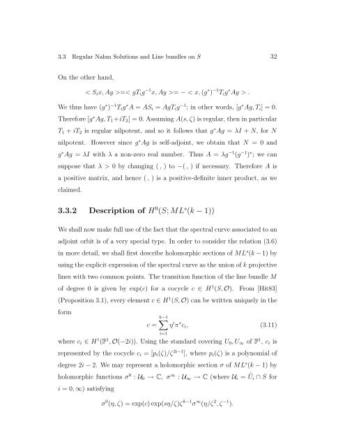
3.3 Regular Nahm Solutions and Line bundles on S 32
On the other hand,
< Six, Ay >=< gTig −1 x, Ay >= − < x, (g ∗ ) −1 Tig ∗ Ay > .
We thus have (g ∗ ) −1 Tig ∗ A = ASi = AgTig −1 ; in other words, [g ∗ Ag, Ti] = 0.
Therefore [g ∗ Ag, T1 +iT2] = 0. Assuming A(s, ζ) is regular, then in particular
T1 + iT2 is regular nilpotent, and so it follows that g ∗ Ag = λI + N, for N
nilpotent. However since g ∗ Ag is self-adjoint, we obtain that N = 0 and
g ∗ Ag = λI with λ a non-zero real number. Thus A = λg −1 (g −1 ) ∗ ; we can
suppose that λ > 0 by changing ( , ) to −( , ) if necessary. Therefore A is
a positive matrix, and hence ( , ) is a positive-definite inner product, as we
claimed.
3.3.2 Description of H 0 (S; ML s (k − 1))
We shall now make full use of the fact that the spectral curve associated to an
adjoint orbit is of a very special type. In order to consider the relation (3.6)
in more detail, we shall first describe holomorphic sections of ML s (k − 1) by
using the explicit expression of the spectral curve as the union of k projective
lines with two common points. The transition function of the line bundle M
of degree 0 is given by exp(c) for a cocycle c ∈ H 1 (S, O). From [Hit83]
(Proposition 3.1), every element c ∈ H 1 (S, O) can be written uniquely in the
form
k−1
c =
i=1
η i π ∗ ci, (3.11)
where ci ∈ H 1 (P 1 , O(−2i)). Using the standard covering U0, U∞ of P 1 , ci is
represented by the cocycle ci = [pi(ζ)/ζ 2i−1 ], where pi(ζ) is a polynomial of
degree 2i − 2. We may represent a holomorphic section σ of ML s (k − 1) by
holomorphic functions σ 0 : U0 → C, σ ∞ : U∞ → C (where Ui = Ũi ∩ S for
i = 0, ∞) satisfying
σ 0 (η, ζ) = exp(c) exp(sη/ζ)ζ k−1 σ ∞ (η/ζ 2 , ζ −1 ).