flow and level measurement - Omega Engineering
flow and level measurement - Omega Engineering
flow and level measurement - Omega Engineering

You also want an ePaper? Increase the reach of your titles
YUMPU automatically turns print PDFs into web optimized ePapers that Google loves.
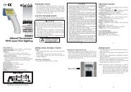
Flow & Level Measurement<br />
A Technical Reference Series Brought to You by OMEGA<br />
VOLUME<br />
4
1<br />
2<br />
3<br />
4<br />
5<br />
TABLE OF CONTENTS<br />
VOLUME 4—FLOW & LEVEL MEASUREMENT<br />
Section Topics Covered Page<br />
A Flow Measurement Orientation<br />
Differential Pressure Flowmeters<br />
Mechanical Flowmeters<br />
Electronic Flowmeters<br />
Mass Flowmeters<br />
• The Flow Pioneers<br />
• Flow Sensor Selection<br />
• Accuracy vs. Repeatability<br />
• Primary Element Options<br />
• Pitot Tubes<br />
• Variable Area Flowmeters<br />
• Positive Displacement Flowmeters<br />
• Turbine Flowmeters<br />
• Other Rotary Flowmeters<br />
• Magnetic Flowmeters<br />
• Vortex Flowmeters<br />
• Ultrasonic Flowmeters<br />
• Coriolis Mass Flowmeters<br />
• Thermal Mass Flowmeters<br />
• Hot-Wire Anemometers<br />
A) Segmental Wedge<br />
Figure 1-3: Faraday's Law is the Basis of the Magnetic Flowmeter<br />
04 Volume 4 TRANSACTIONS<br />
D<br />
Turbulent<br />
Velocity<br />
Flow<br />
Profile<br />
Wedge Flow<br />
Element<br />
or<br />
Laminar<br />
Velocity<br />
Flow<br />
Profile<br />
Figure 2-8: Proprietary Elements For Difficult Fluids<br />
Figure 5-5:<br />
Figure 3-7:<br />
Flanges<br />
Support<br />
A)<br />
C)<br />
Flow<br />
Direction Arrow<br />
H<br />
E<br />
V<br />
B) V-Cone<br />
Calibrated<br />
Volume<br />
H L<br />
1st Detector 2nd Flow Tube<br />
Detector<br />
1.00<br />
0.95<br />
0.90<br />
K<br />
0.85<br />
0.80<br />
0.75<br />
Figure 4-6:<br />
Displacer<br />
Flow<br />
1 10 100 1,000 10 4<br />
0.70<br />
Re<br />
Mass Flowtube<br />
Enclosure<br />
Pipe/Flowtube Junction<br />
NOTE:<br />
Distance Between<br />
Pipe/Flowtube<br />
Junction <strong>and</strong><br />
Support<br />
Must Not<br />
Exceed 15 Inches<br />
'U' Rest 'V' Rest 'V' Bolt<br />
Clamp<br />
K = 0.75 For Laminar Flow<br />
10 5<br />
Support<br />
(Typical)<br />
Mass Tube Enclosure<br />
B)<br />
NOTE: Distance Between<br />
Pipe/Flowtube Junction <strong>and</strong><br />
Support Must Not<br />
Exceed 15 Inches<br />
Inverted Pipe<br />
Hanger Clamp<br />
D<br />
E<br />
K = 1 Asymptote<br />
For Flat Profile<br />
10 6<br />
Magnetic<br />
Coil<br />
10 7<br />
Flow<br />
Direction<br />
Arrow<br />
'V' Block Clamp<br />
(Can Be Inverted)<br />
08<br />
16<br />
34<br />
46<br />
58
6<br />
7<br />
8<br />
9<br />
10<br />
REFERENCE SECTIONS<br />
Editorial 06<br />
About OMEGA 07<br />
• Level Sensor Selection<br />
• Boiling & Cryogenic Fluids<br />
• Sludge, Foam, & Molten Metals<br />
106 Information Resources<br />
110 Glossary<br />
VOLUME 4—FLOW & LEVEL MEASUREMENT<br />
Section Topics Covered Page<br />
A Level Measurement Orientation<br />
Pressure/Density Level Instrumentation<br />
RF/Capacitance Level Instrumentation<br />
Radiation-Based Level Instrumentation<br />
Specialty Level Switches<br />
• Dry & Wet Leg Designs<br />
• Bubbler Tubes<br />
• Floats & Displacers<br />
• Theory of Operation<br />
• Probe Designs<br />
• Installation Considerations<br />
• Radar & Microwave<br />
• Ultrasonic Level Gages<br />
• Nuclear Level Gages<br />
• Thermal Switches<br />
• Vibrating Switches<br />
• Optical Switches<br />
TRANSACTIONS Volume 4 05<br />
A)<br />
Figure 9-6:<br />
A)<br />
Figure 7-3:<br />
Bimetallic<br />
Temperature<br />
Compensator<br />
Reflection<br />
Microwave<br />
Detector<br />
Microwave<br />
Window<br />
High Pressure<br />
Side<br />
Figure 8-2:<br />
Figure 6-3:<br />
Liquid<br />
Fill<br />
Low Pressure<br />
Side<br />
Range<br />
Spring<br />
Level %<br />
100<br />
B)<br />
50<br />
Vertical<br />
Sphere<br />
0<br />
Horizontal<br />
Cylindrical<br />
50<br />
100 Volume %<br />
Nozzle & Flapper<br />
Feedback Bellows<br />
Fulcrum & Seal<br />
Force Bar<br />
Low Pressure<br />
Side<br />
Liquid Filled<br />
Diaphragm<br />
Capsule<br />
-<br />
A) B)<br />
-<br />
- - - -<br />
- -<br />
- -<br />
- - - -<br />
- -<br />
- -<br />
- -<br />
- -<br />
- - - -<br />
-<br />
+ +<br />
+ +<br />
+ +<br />
+ +<br />
+ +<br />
+ +<br />
+ +<br />
+ +<br />
+ +<br />
+ +<br />
+ +<br />
+ +<br />
+ +<br />
+ +<br />
- -<br />
- -<br />
- -<br />
- -<br />
Level<br />
#1<br />
A<br />
A<br />
D<br />
RF<br />
Receiver<br />
Figure 10-4:<br />
Prism<br />
B)<br />
Liquid Below the<br />
Sensing Prism.<br />
Microwave<br />
Transmitter<br />
Microwave<br />
Window<br />
LED<br />
Light<br />
from<br />
LED<br />
Reflected<br />
Beam<br />
Receiver<br />
K v<br />
K l<br />
Voltmeter<br />
Ammeter<br />
Absorbed<br />
Beam<br />
Prism<br />
#2<br />
Transmitted<br />
Beam<br />
Pneumatic<br />
Relay<br />
Output<br />
Electron<br />
Flow<br />
Air<br />
Supply<br />
High Pressure<br />
Side<br />
C= KA D<br />
C=Capacitance<br />
K=Dieletric Constant<br />
A=Area of Plates<br />
D=Dist. Between Plates<br />
Microwave<br />
Receiver<br />
Microwave<br />
Window<br />
Liquid Immersing<br />
the Sensing Prism.<br />
LED<br />
Light<br />
Lost in<br />
Liquid<br />
72<br />
76<br />
87<br />
93<br />
102
1<br />
FLOW & LEVEL MEASUREMENT<br />
A Flow Measurement Orientation<br />
The Flow Pioneers<br />
Flow Sensor Selection<br />
Accuracy vs. Repeatability<br />
O<br />
Our interest in the <strong>measurement</strong><br />
of air <strong>and</strong> water <strong>flow</strong><br />
is timeless. Knowledge of<br />
the direction <strong>and</strong> velocity<br />
of air <strong>flow</strong> was essential information<br />
for all ancient navigators, <strong>and</strong><br />
the ability to measure water <strong>flow</strong><br />
was necessary for the fair distribution<br />
of water through the aqueducts<br />
of such early communities as<br />
Unrecovered Pressure Loss—Percent of Differential<br />
90<br />
80<br />
70<br />
60<br />
50<br />
40<br />
30<br />
20<br />
10<br />
Long Form<br />
Venturi<br />
Low Loss<br />
Venturi<br />
Figure 1-1: Pressure Loss-Venturi vs. Orifice<br />
the Sumerian cities of Ur, Kish, <strong>and</strong><br />
Mari near the Tigris <strong>and</strong> Euphrates<br />
Rivers around 5,000 B.C. Even today,<br />
the distribution of water among the<br />
rice patties of Bali is the sacred<br />
duty of authorities designated the<br />
“Water Priests.”<br />
Our underst<strong>and</strong>ing of the behavior<br />
of liquids <strong>and</strong> gases (including hydro-<br />
A Flow Measurement Orientation<br />
ASME Flow<br />
Nozzle<br />
St<strong>and</strong>ard<br />
Venturi<br />
dynamics, pneumatics, aerodynamics)<br />
is based on the works of the<br />
ancient Greek scientists Aristotle<br />
<strong>and</strong> Archimedes. In the Aristotelian<br />
view, motion involves a medium that<br />
rushes in behind a body to prevent a<br />
vacuum. In the sixth century A.D., John<br />
Philoponos suggested that a body in<br />
motion acquired a property called<br />
impetus, <strong>and</strong> that the body came to<br />
Orifice Plate<br />
Proprietary Flow Tube<br />
0.1 0.2 0.3 0.4 0.5 0.6 0.7 0.8 0.9<br />
Beta (Diameter) Ratio<br />
rest when its impetus died out.<br />
In 1687, the English mathematician<br />
Sir Isaac Newton discovered the law<br />
of universal gravitation. The operation<br />
of angular momentum-type<br />
mass <strong>flow</strong>meters is based directly on<br />
Newton’s second law of angular<br />
motion. In 1742, the French mathematician<br />
Rond d’Alembert proved<br />
that Newton’s third law of motion<br />
applies not only to stationary bodies,<br />
but also to objects in motion.<br />
The Flow Pioneers<br />
A major milestone in the underst<strong>and</strong>ing<br />
of <strong>flow</strong> was reached in 1783 when<br />
the Swiss physicist Daniel Bernoulli<br />
published his Hydrodynamica. In it, he<br />
introduced the concept of the conservation<br />
of energy for fluid <strong>flow</strong>s.<br />
Bernoulli determined that an<br />
increase in the velocity of a <strong>flow</strong>ing<br />
fluid increases its kinetic energy<br />
while decreasing its static energy. It is<br />
for this reason that a <strong>flow</strong> restriction<br />
causes an increase in the <strong>flow</strong>ing<br />
velocity <strong>and</strong> also causes a drop in the<br />
static pressure of the <strong>flow</strong>ing fluid.<br />
The permanent pressure loss<br />
through a <strong>flow</strong>meter is expressed<br />
either as a percentage of the total<br />
pressure drop or in units of velocity<br />
heads, calculated as V2 /2g, where V<br />
is the <strong>flow</strong>ing velocity <strong>and</strong> g is the<br />
gravitational acceleration (32.2<br />
feet/second2 or 9.8 meters/second2 at 60° latitude). For example, if the<br />
velocity of a <strong>flow</strong>ing fluid is 10 ft/s,<br />
the velocity head is 100/64.4 = 1.55 ft.<br />
If the fluid is water, the velocity head<br />
corresponds to 1.55 ft of water (or<br />
0.67 psi). If the fluid is air, then the<br />
velocity head corresponds to the<br />
weight of a 1.55-ft column of air.<br />
The permanent pressure loss<br />
through various <strong>flow</strong> elements can<br />
be expressed as a percentage of the<br />
total pressure drop (Figure 1-1), or it<br />
can be expressed in terms of velocity<br />
heads. The permanent pressure<br />
loss through an orifice is four velocity<br />
heads; through a vortex shedding<br />
sensor, it is two; through positive<br />
08 Volume 4 TRANSACTIONS<br />
10<br />
20<br />
30<br />
40<br />
50<br />
60<br />
70<br />
80<br />
90<br />
Recovery—Percent of Differential
displacement <strong>and</strong> turbine meters,<br />
about one; <strong>and</strong>, through <strong>flow</strong> venturis,<br />
less than 0.5 heads. Therefore, if an orifice<br />
plate (Figure 1-2) with a beta ratio<br />
D<br />
Static Pressure<br />
ΔP RT =ΔP VC<br />
Flow<br />
ΔP FT<br />
(0.35-0.85)D<br />
Figure 1-2: Conversion of Static Pressure Into Kinetic Energy<br />
of 0.3 (diameter of the orifice to that<br />
of the pipe) has an unrecovered<br />
pressure loss of 100 in H 2 O, a venturi<br />
<strong>flow</strong> tube could reduce that pressure<br />
loss to about 12 in H 2 O for the<br />
same <strong>measurement</strong>.<br />
In 1831, the English scientist Michael<br />
Faraday discovered the dynamo when<br />
he noted that, if a copper disk is rotated<br />
between the poles of a permanent<br />
magnet, electric current is generated.<br />
Faraday’s law of electromagnetic<br />
induction is the basis for the operation<br />
of the magnetic <strong>flow</strong>meter. As shown<br />
in Figure 1-3, when a liquid conductor<br />
moves in a pipe having a diameter (D)<br />
<strong>and</strong> travels with an average velocity (V)<br />
through a magnetic field of B intensity,<br />
it will induce a voltage (E) according to<br />
the relationship:<br />
E = BVDC<br />
ΔP CT<br />
where C is the constant for units<br />
conversion.<br />
Over the past several years, the<br />
performance of magnetic <strong>flow</strong>meters<br />
Unstable Region, No Pressure<br />
Tap Can Be Located Here<br />
Pressure at Vena Contracta (P VC )<br />
Minimum Diameter<br />
2.5D<br />
D D/2<br />
8D<br />
Corner Taps (CT), D ‹ 2"<br />
Orifice<br />
Flange Taps (FT), D › 2"<br />
Radius Taps (RT), D › 6"<br />
Pipe Taps (PT)<br />
has improved significantly. Among the<br />
advances are probe <strong>and</strong> ceramic insert<br />
designs <strong>and</strong> the use of pulsed magnetic<br />
fields (Figure 1-4), but the basic<br />
operating principle of Faraday’s law of<br />
electric induction has not changed.<br />
In 1883, the British mechanical engineer<br />
Osborne Reynolds proposed a<br />
Turbulent<br />
Velocity<br />
Flow<br />
Profile<br />
or<br />
1 A Flow Measurement Orientation<br />
single, dimensionless ratio to describe<br />
the velocity profile of <strong>flow</strong>ing fluids:<br />
Re = DVρ/μ<br />
Where D is the pipe diameter, V is<br />
the fluid velocity, ρ is the fluid density,<br />
<strong>and</strong> μ is the fluid viscosity.<br />
He noted that, at low Reynolds<br />
numbers (below 2,000) (Figure 1-5),<br />
<strong>flow</strong> is dominated by viscous forces<br />
<strong>and</strong> the velocity profile is (elongated)<br />
parabolic. At high Reynolds numbers<br />
(above 20,000), the <strong>flow</strong> is dominated<br />
by inertial forces, resulting in a more<br />
uniform axial velocity across the <strong>flow</strong>ing<br />
stream <strong>and</strong> a flat velocity profile.<br />
Until 1970 or so, it was believed<br />
that the transition between laminar<br />
<strong>and</strong> turbulent <strong>flow</strong>s is gradual, but<br />
increased underst<strong>and</strong>ing of turbulence<br />
through supercomputer modeling<br />
has shown that the onset of<br />
turbulence is abrupt.<br />
When <strong>flow</strong> is turbulent, the pressure<br />
drop through a restriction is<br />
proportional to the square of the<br />
<strong>flow</strong>rate. Therefore, <strong>flow</strong> can be<br />
measured by taking the square root<br />
of a differential pressure cell output.<br />
When the <strong>flow</strong> is laminar, a linear<br />
relationship exists between <strong>flow</strong> <strong>and</strong><br />
pressure drop. Laminar <strong>flow</strong>meters<br />
TRANSACTIONS Volume 4 09<br />
Flow<br />
Laminar<br />
Velocity<br />
Flow<br />
Profile<br />
ΔP PT<br />
Figure 1-3: Faraday's Law Is the Basis of the Magnetic Flowmeter<br />
E<br />
V<br />
D<br />
E<br />
Magnetic<br />
Coil
A Flow Measurement Orientation<br />
are used at very low <strong>flow</strong>rates (capillary<br />
<strong>flow</strong>meters) or when the viscosity<br />
of the process fluid is high.<br />
In the case of some <strong>flow</strong>meter<br />
technologies, more than a century<br />
elapsed between the discovery of a<br />
% Rate Accuracy<br />
4.0<br />
3.0<br />
2.0<br />
1.0<br />
0.5<br />
0<br />
-0.5<br />
-1.0<br />
-2.0<br />
-3.0<br />
-4.0<br />
Conventional<br />
Magnetic Flowmeters<br />
Performance of Pulsed<br />
DC Magnetic Flowmeters<br />
10 50 100<br />
% Full Scale<br />
Figure 1-4: Magmeter Accuracy<br />
scientific principle <strong>and</strong> its use in<br />
building a <strong>flow</strong>meter. This is the case<br />
with both the Doppler ultrasonic <strong>and</strong><br />
the Coriolis meter.<br />
In 1842, the Austrian physicist<br />
Christian Doppler discovered that, if a<br />
sound source is approaching a receiver<br />
(such as a train moving toward a stationary<br />
listener), the frequency of the<br />
sound will appear higher. If the source<br />
<strong>and</strong> the recipient are moving away<br />
from each other, the pitch will drop<br />
(the wavelength of the sound will<br />
appear to decrease). Yet it was more<br />
than a century later that the first ultrasonic<br />
Doppler <strong>flow</strong>meter came on the<br />
market. It projected a 0.5-MHz beam<br />
into a <strong>flow</strong>ing stream containing reflectors<br />
such as bubbles or particles. The<br />
shift in the reflected frequency was a<br />
function of the average traveling velocity<br />
of the reflectors. This speed, in turn,<br />
could be used to calculate a <strong>flow</strong>rate.<br />
The history of the Coriolis<br />
1<br />
<strong>flow</strong>meter is similar. The French civil<br />
engineer Gaspard Coriolis discovered<br />
in 1843 that the wind, the ocean currents,<br />
<strong>and</strong> even airborne artillery<br />
shells will all drift sideways because<br />
of the earth’s rotation. In the northern<br />
hemisphere, the deflection is to the<br />
right of the motion; in the southern<br />
hemisphere, it is to the left. Similarly,<br />
a body traveling toward either pole<br />
will veer eastward, because it retains<br />
the greater eastward rotational speed<br />
of the lower altitudes as it passes<br />
over the more slowly rotating earth<br />
surface near the poles. Again, it was<br />
the slow evolution of sensors <strong>and</strong><br />
electronics that delayed creation of<br />
the first commercial Coriolis mass<br />
<strong>flow</strong>meter until the 1970’s.<br />
It was the Hungarian-American<br />
aeronautical engineer Theodore<br />
von Karman who, as a child growing<br />
up in Transylvania (now Romania),<br />
noticed that stationary rocks caused<br />
vortices in <strong>flow</strong>ing water, <strong>and</strong> that<br />
the distances between these traveling<br />
vortices are constant, no matter<br />
how fast or slow the water runs.<br />
Later in life, he also observed that,<br />
when a flag flutters in the wind, the<br />
wavelength of the flutter is independent<br />
of wind velocity <strong>and</strong> depends<br />
solely on the diameter of the flag<br />
pole. This is the theory behind the<br />
vortex <strong>flow</strong>meter, which determines<br />
<strong>flow</strong> velocity by counting the number<br />
of vortices passing a sensor. Von<br />
Karman published his findings in<br />
1954, <strong>and</strong> because by that time the<br />
sensors <strong>and</strong> electronics required to<br />
count vortices were already in existence,<br />
the first edition of the<br />
Instrument Engineers’ H<strong>and</strong>book in<br />
1968 was able to report the availability<br />
of the first swirlmeter.<br />
The computer has opened new<br />
frontiers in all fields of engineering,<br />
<strong>and</strong> <strong>flow</strong> <strong>measurement</strong> is no exception.<br />
It was only as long ago as 1954<br />
that another Hungarian-American<br />
mathematician, John Von Neumann,<br />
built Uniac—<strong>and</strong> even more recently<br />
that yet another Hungarian-<br />
American, Andy Grove of Intel,<br />
developed the integrated circuit. Yet<br />
these events are already changing<br />
the field of <strong>flow</strong>metering. Intelligent<br />
differential pressure cells, for example,<br />
can automatically switch their<br />
range between two calibrated spans<br />
(one for 1-10%, the other for 10-100%<br />
of D/P), extending orifice accuracy<br />
to within 1% over a 10:1 <strong>flow</strong> range.<br />
Furthermore, it is possible to include<br />
in this accuracy statement not only<br />
hysteresis, rangeability, <strong>and</strong> linearity<br />
Flow <strong>measurement</strong> options run the gamut from simple, economical paddle wheels (shown) to<br />
sophisticated high-accuracy devices.<br />
effects, but also drift, temperature,<br />
humidity, vibration, over-range, <strong>and</strong><br />
10 Volume 4 TRANSACTIONS
power supply variation effects.<br />
With the development of superchips,<br />
the design of the universal<br />
<strong>flow</strong>meter also has become feasible.<br />
It is now possible to replace dyetagging<br />
or chemical-tracing meters<br />
(which measured <strong>flow</strong> velocity by<br />
dividing the distance between two<br />
points by the transit time of the<br />
trace), with traceless cross-correlation<br />
<strong>flow</strong>meters (Figure 1-6). This is<br />
an elegant <strong>flow</strong>meter because it<br />
requires no physical change in the<br />
process—not even penetration of<br />
the pipe. The <strong>measurement</strong> is based<br />
on memorizing the noise pattern in<br />
any externally detectable process<br />
variable, <strong>and</strong>, as the fluid travels<br />
from point A to point B, noting its<br />
transit time.<br />
Flow Sensor Selection<br />
The purpose of this section is to<br />
provide information to assist the<br />
reader in making an informed selection<br />
of <strong>flow</strong>meter for a particular<br />
application. Selection <strong>and</strong> orientation<br />
tables are used to quickly focus<br />
on the most likely c<strong>and</strong>idates for<br />
<strong>measurement</strong>. Tables 1-I <strong>and</strong> 1-II<br />
have been prepared to make available<br />
a large amount of information<br />
for this selection process.<br />
At this point, one should consider<br />
such intangible factors as familiarity of<br />
plant personnel, their experience with<br />
calibration <strong>and</strong> maintenance, spare<br />
parts availability, mean time between<br />
failure history, etc., at the particular<br />
plant site. It is also recommended that<br />
the cost of the installation be computed<br />
only after taking these steps. One<br />
of the most common <strong>flow</strong> <strong>measurement</strong><br />
mistakes is the reversal of this<br />
sequence: instead of selecting a sensor<br />
which will perform properly, an<br />
attempt is made to justify the use of a<br />
device because it is less expensive.<br />
Those “inexpensive” purchases can be<br />
the most costly installations.<br />
The basis of good <strong>flow</strong>meter<br />
selection is a clear underst<strong>and</strong>ing of<br />
the requirements of the particular<br />
application. Therefore, time should<br />
be invested in fully evaluating the<br />
nature of the process fluid <strong>and</strong> of the<br />
overall installation. The development<br />
of specifications that state the appli-<br />
Coefficient of Discharge<br />
Target Meter<br />
(Best Case)<br />
10 10 2<br />
Figure 1-5: Effect of Reynolds Numbers on Various Flowmeters<br />
cation requirements should be a systematic,<br />
step-by-step process.<br />
The first step in the <strong>flow</strong> sensor<br />
selection process is to determine if<br />
the <strong>flow</strong>rate information should be<br />
continuous or totalized, <strong>and</strong> whether<br />
this information is needed locally or<br />
remotely. If remotely, should the<br />
transmission be analog, digital, or<br />
shared? And, if shared, what is the<br />
required (minimum) data-update frequency?<br />
Once these questions are<br />
answered, an evaluation of the properties<br />
<strong>and</strong> <strong>flow</strong> characteristics of the<br />
process fluid, <strong>and</strong> of the piping that<br />
will accommodate the <strong>flow</strong>meter,<br />
should take place (Table 1-I). In order<br />
to approach this task in a systematic<br />
manner, forms have been developed,<br />
requiring that the following types of<br />
1 A Flow Measurement Orientation<br />
data be filled in for each application:<br />
• Fluid <strong>and</strong> <strong>flow</strong> characteristics: In<br />
this section of the table, the name<br />
of the fluid is given <strong>and</strong> its pressure,<br />
temperature, allowable pressure<br />
drop, density (or specific gravity),<br />
conductivity, viscosity (Newtonian<br />
or not?) <strong>and</strong> vapor pressure at<br />
maximum operating temperature<br />
are listed, together with an indica-<br />
tion of how these properties<br />
might vary or interact. In addition,<br />
all safety or toxicity information<br />
should be provided, together with<br />
detailed data on the fluid’s composition,<br />
presence of bubbles, solids<br />
(abrasive or soft, size of particles,<br />
fibers), tendency to coat, <strong>and</strong> light<br />
transmission qualities (opaque,<br />
translucent or transparent?).<br />
• Expected minimum <strong>and</strong> maximum<br />
pressure <strong>and</strong> temperature values<br />
should be given in addition to the<br />
normal operating values. Whether<br />
<strong>flow</strong> can reverse, whether it does<br />
not always fill the pipe, whether<br />
slug <strong>flow</strong> can develop (air-solids-liquid),<br />
whether aeration or pulsation<br />
is likely, whether sudden temperature<br />
changes can occur, or whether<br />
TRANSACTIONS Volume 4 11<br />
10 3<br />
Concentric<br />
Square-Edged<br />
Orifice<br />
Integral<br />
Orifice<br />
10 4<br />
Eccentric<br />
Orifice<br />
Flow<br />
Nozzle<br />
Target Meter<br />
Magnetic<br />
Flowmeter<br />
Venturi Tube<br />
(Worst Case) Quadrant-Edged<br />
Orifice<br />
10 5<br />
10 6<br />
Pipeline<br />
Reynolds<br />
Number
A Flow Measurement Orientation<br />
special precautions are needed during<br />
cleaning <strong>and</strong> maintenance, these<br />
facts, too, should be stated.<br />
• Concerning the piping <strong>and</strong> the area<br />
where the <strong>flow</strong>meter is to be located,<br />
the following information<br />
m(t)<br />
n(t)<br />
should be specified: For the piping,<br />
its direction (avoid downward <strong>flow</strong><br />
in liquid applications), size, material,<br />
schedule, flange-pressure rating,<br />
accessibility, up or downstream<br />
turns, valves, regulators, <strong>and</strong> available<br />
straight-pipe run lengths.<br />
• In connection with the area, the<br />
specifying engineer must know if<br />
vibration or magnetic fields are present<br />
or possible, if electric or pneumatic<br />
power is available, if the area<br />
is classified for explosion hazards,<br />
or if there are other special<br />
requirements such as compliance<br />
1<br />
m(t)<br />
A<br />
Transit<br />
Time<br />
n(t)<br />
Figure 1-6: The Ultrasonic Transit-Time Flowmeter<br />
B<br />
with sanitary or clean-in-place<br />
(CIP) regulations.<br />
The next step is to determine the<br />
required meter range by identifying<br />
minimum <strong>and</strong> maximum <strong>flow</strong>s (mass<br />
or volumetric) that will be measured.<br />
Transport Pipe<br />
Position A Position B<br />
Time Delay<br />
Flow<br />
Upstream<br />
Transducer Signal<br />
Time. t<br />
Downstream<br />
Transducer Signal<br />
Time. t<br />
After that, the required <strong>flow</strong> <strong>measurement</strong><br />
accuracy is determined.<br />
Typically accuracy is specified in percentage<br />
of actual reading (AR), in<br />
percentage of calibrated span (CS), or<br />
in percentage of full scale (FS) units.<br />
The accuracy requirements should be<br />
separately stated at minimum, normal,<br />
<strong>and</strong> maximum <strong>flow</strong>rates. Unless<br />
you know these requirements, your<br />
meter’s performance may not be<br />
acceptable over its full range.<br />
Accuracy vs. Repeatability<br />
In applications where products are<br />
sold or purchased on the basis of a<br />
meter reading, absolute accuracy is<br />
critical. In other applications,<br />
repeatability may be more important<br />
than absolute accuracy. Therefore, it<br />
is advisable to establish separately<br />
the accuracy <strong>and</strong> repeatability<br />
requirements of each application <strong>and</strong><br />
to state both in the specifications.<br />
When a <strong>flow</strong>meter’s accuracy is<br />
stated in % CS or % FS units, its<br />
absolute error will rise as the measured<br />
<strong>flow</strong> rate drops. If meter error is<br />
stated in % AR, the error in absolute<br />
terms stays the same at high or low<br />
<strong>flow</strong>s. Because full scale (FS) is always<br />
a larger quantity than the calibrated<br />
span (CS), a sensor with a % FS performance<br />
will always have a larger error<br />
than one with the same % CS specification.<br />
Therefore, in order to compare<br />
all bids fairly, it is advisable to convert<br />
all quoted error statements into the<br />
same % AR units.<br />
It is also recommended that the<br />
user compare installations on the<br />
basis of the total error of the loop. For<br />
example, the inaccuracy of an orifice<br />
plate is stated in % AR, while the error<br />
of the associated d/p cell is in % CS<br />
or % FS. Similarly, the inaccuracy of a<br />
Coriolis meter is the sum of two<br />
errors, one given in % AR, the other as<br />
a % FS value. Total inaccuracy is calculated<br />
by taking the root of the sum of<br />
the squares of the component inaccuracies<br />
at the desired <strong>flow</strong> rates.<br />
In well-prepared <strong>flow</strong>meter specifications,<br />
all accuracy statements are<br />
converted into uniform % AR units <strong>and</strong><br />
these % AR requirements are specified<br />
separately for minimum, normal, <strong>and</strong><br />
maximum <strong>flow</strong>s. All <strong>flow</strong>meter specifications<br />
<strong>and</strong> bids should clearly state<br />
both the accuracy <strong>and</strong> the repeatability<br />
of the meter at minimum, normal,<br />
<strong>and</strong> maximum <strong>flow</strong>s.<br />
Table 1 provides data on the range<br />
12 Volume 4 TRANSACTIONS
of Reynolds numbers (Re or R D ) within<br />
which the various <strong>flow</strong>meter<br />
designs can operate. In selecting the<br />
right <strong>flow</strong>meter, one of the first steps<br />
is to determine both the minimum<br />
<strong>and</strong> the maximum Reynolds numbers<br />
for the application. Maximum R D is<br />
obtained by making the calculation<br />
Table 1: Flowmeter Evaluation Table<br />
FLOWMETER PIPE SIZE, in. (mm)<br />
SQUARE ROOT SCALE: MAXIMUM SINGLE RANGE 4:1 (Typical)**<br />
Orifice<br />
Square-Edged<br />
Honed Meter Run<br />
Integrated<br />
Segmental Wedge<br />
Eccentric<br />
Segmental<br />
V-Cone<br />
Target***<br />
Venturi<br />
Flow Nozzle<br />
Low Loss Venturi<br />
Pitot<br />
Averaging Pitot<br />
Elbow<br />
Laminar<br />
Magnetic*<br />
Positive Displacement<br />
Gas<br />
Liquid<br />
Turbine<br />
Gas<br />
Liquid<br />
Ultrasonic<br />
Time of Flight<br />
Doppler<br />
Variable-Area (Rotameter)<br />
Vortex Shedding<br />
Vortex Precession (Swirl)<br />
Fluidic Oscillation (Co<strong>and</strong>a)<br />
Mass<br />
Coriolis<br />
Thermal Probe<br />
Solids Flowmeter<br />
Correlation<br />
Capacitance<br />
Ultrasonic<br />
cP = centi Poise<br />
cS = centi Stokes<br />
SD = Some designs<br />
>1.5 (40)<br />
0.5-1.5 (12-40)<br />
4 (100)<br />
0.5-72 (12-1800)<br />
2 (50)<br />
>2 (50)<br />
>3 (75)<br />
>3 (75)<br />
>1 (25)<br />
>2 (50)<br />
0.25-16.6 (6-400)<br />
0.5 (12)<br />
≤3 (75)<br />
1.5-16 (40-400)<br />
1.5 (40)<br />
0.25-6 (6-150)<br />
10,000<br />
R D > 10,000<br />
R D > 500<br />
R D > 10,000<br />
R D > 10,000<br />
R D : 8,000-5,000,000<br />
R D > 100<br />
R D > 75,000Ł<br />
R D > 50,000Ł<br />
R D > 12,800Ł<br />
R D > 100,000Ł<br />
R D > 40,000Ł<br />
R D > 10,000Ł<br />
R D < 500<br />
‡ According to other sources, the minimum<br />
Reynolds number should be much higher<br />
* Liquid must be electrically conductive<br />
** Range 10:1 for laminar, <strong>and</strong> 15:1 for target<br />
*** Newer designs linearize the signal<br />
TRANSACTIONS Volume 4 13<br />
?<br />
X<br />
X<br />
X<br />
X<br />
X<br />
?<br />
X<br />
X<br />
X<br />
X<br />
√<br />
?<br />
X<br />
?<br />
?<br />
X<br />
X<br />
X<br />
X<br />
X<br />
X<br />
X<br />
X<br />
X<br />
X<br />
X<br />
X<br />
X<br />
X<br />
X<br />
?<br />
X<br />
X<br />
?<br />
?<br />
?<br />
X<br />
X<br />
X<br />
X<br />
X<br />
X<br />
X<br />
X<br />
X<br />
X<br />
TYPICAL<br />
Accuracy, uncalibrated<br />
(Including transmitter)<br />
±1-4% URV<br />
±1% URV<br />
±2-5% URV<br />
±0.5% URV<br />
±2-4% URV<br />
±2-4% URV<br />
±0.5-1% of rate<br />
±0.5-5% URV<br />
±0.5-2% URV<br />
±1-2% URV<br />
±1.25% URV<br />
±3-5% URV<br />
±1-2% URV<br />
±5-10% URV<br />
±1% of rate<br />
±0.5% of rate<br />
±1% of rate<br />
±0.5% of rate<br />
±0.5% of rate<br />
±0.5% of rate<br />
±1% of rate to ±5% URV<br />
±1% of rate to ±5% URV<br />
±1% of rate to ±10% URV<br />
±0.75-1.5% of rate<br />
±0.5% of rate<br />
±2% of rate<br />
±0.15-10% of rate<br />
±1-2% URV<br />
±0.5% of rate to ±4% URV<br />
No data available<br />
±6% of ??<br />
TYPICAL<br />
Reynolds number ‡<br />
or viscosity<br />
R D > 4,500<br />
-<br />
No R D limit ≤ 8,000 cS<br />
-<br />
Rp > 5,000, ≤15 cS<br />
R D > 10,000<br />
R D > 4,000<br />
No R D limit, < 100 cS<br />
R D > 10,000, < 30 cP<br />
R D > 10,000, < 5 cP<br />
R D > 2,000, < 80 cS<br />
No R D limit<br />
No R D limit<br />
-<br />
No data available<br />
No data available<br />
TEMPERATURE<br />
°F (°C)<br />
Process temperature<br />
to 1000°F (540°C):<br />
Transmitter limited<br />
to -30-250°F (-30-120°C)<br />
700 (370)<br />
Process temperature<br />
to 1000°F (540°C):<br />
Transmitter limited<br />
to -30-250°F (-30-120°C)<br />
150 (66)<br />
360 (180)<br />
250 (120)<br />
600 (315)<br />
-450-500 (268-260)<br />
-450-500 (268-260)<br />
-300-500 (-180-260)<br />
-300-500 (-180-260)<br />
Glass: 400 (200)<br />
Metal: 1,000 (540)<br />
400 (200)<br />
536 (280)<br />
350 (175)<br />
-400-800 (-224-427)<br />
1,500 (816)<br />
750 (400)<br />
300 (149)<br />
-300-250 (-180-120)<br />
PRESSURE<br />
psig (kPa)<br />
To 4,000 psig<br />
(41,000 kPa)<br />
≤600 (4,100)<br />
To 4,000 psig<br />
(41,000 kPa)<br />
≤30 (225)<br />
≤ 1,500 (10,800)<br />
≤ 1,400 (10,000)<br />
≤ 1,400 (10,000)<br />
≤ 3,000 (21,000)<br />
≤ 3,000 (21,000)<br />
Pipe rating<br />
Pipe rating<br />
Glass: 350 (2,400)<br />
Metal: 720 (5,000)<br />
≤ 1,500 (10,500)<br />
Pipe rating<br />
≤ 720 (5,000)<br />
≤ 5,700 (39,900)<br />
Pipe rating<br />
≤ 580 (4,000)<br />
≤ 580 (4,000)<br />
Pipe rating
A Flow Measurement Orientation<br />
TYPE OF DESIGN<br />
the <strong>flow</strong> being measured. Even<br />
with well maintained <strong>and</strong> calibrated<br />
meters, this unmeasured <strong>flow</strong> varies<br />
with changes in fluid viscosity <strong>and</strong><br />
temperature. Changes in temperature<br />
Table 2: Orientation Table For Flow Sensors<br />
Orifice (plate or integral cell) √<br />
Segmental Wedge<br />
√<br />
V-Cone Flowmeter<br />
√<br />
Target Meters<br />
√<br />
Venturi Tubes<br />
√<br />
Flow Nozzles<br />
√<br />
Pitot Tubes<br />
√<br />
Elbow Taps<br />
√<br />
Laminar Flowmeters<br />
√<br />
Magnetic Flowmeters<br />
Positive Displacement<br />
Gas Meters<br />
Positive Displacement<br />
Liquid Meters<br />
Turbine Flowmeters<br />
Ultrasonic Flowmeters<br />
Time of Flight<br />
Doppler<br />
Variable Area (Rotamater)<br />
Vortex Shedding<br />
SD<br />
Fluidic Oscillation (Co<strong>and</strong>a)<br />
Mass Flowmeters Coriolis √<br />
Mass Flowmeters<br />
√<br />
Thermal Probe<br />
Solids Flowmeters<br />
SD<br />
Weirs, Flumes<br />
= Non-st<strong>and</strong>ard Range<br />
L = Limited<br />
SD = Some Designs<br />
H = High<br />
A = Average<br />
M = Minimal<br />
N = None<br />
SR = Square Root<br />
DIRECT MASS-FLOW SENSOR<br />
DIFFERENTIAL PRESSURE-FLOW SENSOR<br />
VOLUME DISPLACEMENT-FLOW SENSOR<br />
VELOCITY-FLOW SENSOR<br />
EXPECTED ERROR FROM VISCOSITY CHANGE<br />
TRANSMITTER AVAILABLE<br />
LINEAR OUTPUT<br />
RANGEABILITY<br />
√<br />
√<br />
√<br />
√<br />
√<br />
√<br />
√<br />
√<br />
√<br />
√<br />
√<br />
SD<br />
1<br />
H √<br />
➁<br />
SR 3:1 H 20/5<br />
M √ SR 3:1<br />
➁<br />
A 20/5<br />
√<br />
➁<br />
SR 3:1 to 15:1 M 2/5<br />
A √ SR 15:1 M 20/5<br />
H √ SR 3:1 ➁ M 15/5<br />
H √ SR 3:1 ➁<br />
A 20/5<br />
M √ SR 3:1 ➁ M 30/5<br />
M √ SR 3:1<br />
➁<br />
N 25/10<br />
√ √ 10:1<br />
➁<br />
H 15/5<br />
N √ √ 30:1<br />
➆<br />
N 5/3<br />
SD √ 10:1 to<br />
200:1<br />
M N<br />
M SD √<br />
➆<br />
10:1 A N<br />
H<br />
N<br />
N<br />
A<br />
A<br />
A<br />
N<br />
N<br />
M<br />
√<br />
√<br />
√ √<br />
√ √<br />
√ √<br />
√ √<br />
√ √<br />
√ √<br />
√ √<br />
10:1<br />
➇<br />
20:1<br />
10:1<br />
10:1<br />
10/1<br />
➅<br />
12/1➅<br />
20:1<br />
20:1➆<br />
PRESSURE LOSS THRU SENSOR<br />
A<br />
N<br />
N<br />
M<br />
A<br />
H<br />
M/H<br />
M<br />
also change the internal dimensions of<br />
the meter <strong>and</strong> require compensation.<br />
Furthermore, if one can obtain the<br />
same performance from both a full<br />
<strong>flow</strong>meter <strong>and</strong> a point sensor, it is<br />
APPROX. STRAIGHT PIPE-RUN REQUIREMENT ➀➄<br />
(UPSTREAM DIAM./DOWNSTREAM DIAM.)<br />
15/5<br />
20/5<br />
20/5<br />
N<br />
20/5<br />
20/5<br />
N<br />
20/5<br />
√ √ 5:1 to 80:1 - 5/3<br />
√ SD 100:1 M 4/1<br />
0.05 0.3 2.8 28.3<br />
➀ = The data in this column is for general guidance only.<br />
➁ = Inherent rangeability of primary device is substantially greater than shown. Value used reflects<br />
limitations of differential pressure sensing device when 1% of rate accuracy is desired. With<br />
multiple-range intelligent transmitters, rangeability can reach 10:1.<br />
➂ = Pipe size establishes the upper limit.<br />
➃ = Practically unlimited with probe type design.<br />
generally advisable to use the<br />
<strong>flow</strong>meter. Because point sensors do<br />
not look at the full <strong>flow</strong>, they read<br />
accurately only if they are inserted to<br />
a depth where the <strong>flow</strong> velocity is<br />
FLOW RANGE➈<br />
0.1 1.0 10 10 2<br />
0.1 1.0 10 10 2<br />
14 Volume 4 TRANSACTIONS<br />
10 -6<br />
10 -6<br />
10 -5<br />
10 -5<br />
10 -4<br />
10 -4<br />
10 -3<br />
10 -3<br />
cc/min<br />
10 -2<br />
.004 0.04 0.4 3.8 38 379<br />
10 -6<br />
10 -6<br />
10 -5<br />
10 -5<br />
10 -4<br />
10 -4<br />
10 -3<br />
10 -3<br />
10 -2<br />
10 -2<br />
0.1<br />
10 -2<br />
0.1<br />
0.1 1.0<br />
cc/min<br />
0.1<br />
1.0<br />
1.0<br />
10<br />
1.0<br />
10<br />
10<br />
10 2<br />
10<br />
10 2<br />
10 2<br />
10 3<br />
10 3<br />
10 4<br />
Sm 3 /hr or Am 3 /hr<br />
10 3<br />
10 2<br />
10 3<br />
10 3<br />
10 4<br />
10 3<br />
10 4 kgm/hr<br />
10 4<br />
10 4<br />
10 5<br />
10 4<br />
m 3 /hr<br />
10 5<br />
10 5<br />
gpm—m 3 /hr<br />
10 6<br />
10 6<br />
gpm<br />
Solids<br />
Flow<br />
Units<br />
Gas<br />
Flow<br />
Units<br />
Liquid<br />
Flow<br />
Units<br />
gpm—m 3 /hr<br />
SCFM—Sm 3 ➂<br />
/hr<br />
gpm—m 3 /hr<br />
ACFM—Sm 3 /hr<br />
gpm—m 3 /hr<br />
SCFM—Sm 3 ➃<br />
/hr<br />
gpm—m 3 /hr<br />
SCFM—Sm 3 /hr<br />
gpm—m 3 gpm—m<br />
/hr<br />
3 /hr<br />
SCFM—Sm 3 /hr<br />
gpm—m 3 /hr<br />
SCFM—Sm 3 /hr<br />
gpm—m 3 /hr<br />
SCFM—Sm 3 ➃<br />
➂<br />
/hr<br />
SCFM—Sm 3 /hr<br />
gpm—m 3 /hr<br />
gpm—m 3 /hr<br />
SCFM—Sm 3 /hr<br />
gpm—m 3 /hr<br />
SCFM—Sm 3 /hr<br />
gpm—m 3 /hr<br />
SCFM—Sm 3 ➂<br />
/hr<br />
gpm—m 3 /hr<br />
ACFM—Sm 3 /hr<br />
gpm—m 3 /hr<br />
SCFM—Sm 3 SCFM—Sm<br />
/hr<br />
3 /hr<br />
lbm—kgm/hr<br />
gpm—m 3 lbm—kgm/hr<br />
/hr<br />
➄ = Varies with upstream disturbance.<br />
➅ = Can be more with high Reynolds number services.<br />
➆ = Up to 100:1.<br />
➇ = More for gas turbine meters.<br />
➈ = Higher <strong>and</strong> lower <strong>flow</strong> ranges may be available.<br />
Check several manufacturers.<br />
➂<br />
➂
the average of the velocity profile<br />
across the pipe. Even if this point is<br />
carefully determined at the time of<br />
calibration, it is not likely to remain<br />
unaltered, since velocity profiles<br />
change with <strong>flow</strong>rate, viscosity, temperature,<br />
<strong>and</strong> other factors.<br />
If all other considerations are the<br />
same, but one design offers less pressure<br />
loss, it is advisable to select that<br />
design. Part of the reason is that the<br />
pressure loss will have to be paid for<br />
in higher pump or compressor operating<br />
costs over the life of the plant.<br />
Another reason is that a pressure drop<br />
is caused by any restriction in the <strong>flow</strong><br />
path, <strong>and</strong> wherever a pipe is restricted<br />
becomes a potential site for material<br />
build-up, plugging, or cavitation.<br />
Before specifying a <strong>flow</strong>meter, it is<br />
also advisable to determine whether<br />
the <strong>flow</strong> information will be more useful<br />
if presented in mass or volumetric<br />
units. When measuring the <strong>flow</strong> of<br />
compressible materials, volumetric<br />
<strong>flow</strong> is not very meaningful unless<br />
density (<strong>and</strong> sometimes also viscosity)<br />
is constant. When the velocity (volumetric<br />
<strong>flow</strong>) of incompressible liquids<br />
is measured, the presence of suspended<br />
bubbles will cause error; therefore,<br />
air <strong>and</strong> gas must be removed before<br />
the fluid reaches the meter. In other<br />
velocity sensors, pipe liners can cause<br />
problems (ultrasonic), or the meter<br />
may stop functioning if the Reynolds<br />
number is too low (in vortex shedding<br />
meters, R D > 20,000 is required).<br />
In view of these considerations,<br />
mass <strong>flow</strong>meters, which are insensitive<br />
to density, pressure <strong>and</strong> viscosity variations<br />
<strong>and</strong> are not affected by changes<br />
in the Reynolds number, should be<br />
kept in mind. Also underutilized in the<br />
chemical industry are the various<br />
flumes that can measure <strong>flow</strong> in partially<br />
full pipes <strong>and</strong> can pass large<br />
floating or settlable solids. T<br />
1 A Flow Measurement Orientation<br />
References & Further Reading<br />
• OMEGA Complete Flow <strong>and</strong> Level Measurement H<strong>and</strong>book <strong>and</strong><br />
Encyclopedia®, OMEGA Press, 1995.<br />
• OMEGA Volume 29 H<strong>and</strong>book & Encyclopedia, Purchasing Agents<br />
Edition, OMEGA Press, 1995.<br />
• “Advanced Process Control for Two-Phase Mixtures,” David Day,<br />
Christopher Reiner <strong>and</strong> Michael Pepe, Measurements & Control, June, 1997.<br />
• Applied Fluid Flow Measurement, N.P. Cheremisinoff, Marcel Decker, 1979.<br />
• “Characteristics <strong>and</strong> Applications of Industrial Thermal Mass Flow<br />
Transmitters,” Jerome L. Kurz, Proceedings 47th Annual Symposium on<br />
Instrumentation for the Process Industries, ISA, 1992.<br />
• Developments in Thermal Flow Sensors, Jerome L. Kurz, Ph.D., Kurz<br />
Instruments Inc., 1987.<br />
• “Differential Flow Measurement of Meter-Conditioned Flow,” Stephen A.<br />
Ifft <strong>and</strong> Andrew J. Zacharias, Measurements & Control, September, 1993.<br />
• Dry Solids Flow Update, Auburn International Inc.<br />
• Flow Measurement <strong>Engineering</strong> H<strong>and</strong>book, R.W. Miller, McGraw-Hill, 1983.<br />
• Flow Measurement for Engineers <strong>and</strong> Scientists, N.P. Cheremisinoff,<br />
Marcel Dekker, 1988.<br />
• Flow Measurement, Bela Liptak, CRC Press, 1993.<br />
• “Flowmeter Geometry Improves Measurement Accuracy,” Stephen A.<br />
Ifft, Measurements & Control, October, 1995.<br />
• Flowmeters, F. Cascetta, P. Vigo, ISA, 1990.<br />
• Fluidic Flowmeter, Bulletin 1400 MX, Moore Products Co., June, 1988.<br />
• Fundamentals of Flow Metering, Technical Data Sheet 3031, Rosemount<br />
Inc., 1982.<br />
• Guide to Variable Area Flowmeters, Application No.: T-022 Issue I,<br />
Brooks Instrument Co., 1986.<br />
• Incompressible Flow, Donald Panton, Wiley, 1996.<br />
• Industrial Flow Measurement, D.W. Spitzer, ISA, 1984.<br />
• “Installation Effects on Venturi Tube Flowmeters”, G. Kochen, D.J.M.<br />
Smith, <strong>and</strong> H. Umbach, Intech, October, 1989.<br />
• Instrument Engineers’ H<strong>and</strong>book, Bela Liptak, ed., CRC Press, 1995.<br />
• “Is a Turbine Flowmeter Right for Your Application?” Michael Hammond,<br />
Flow Control, April, 1998.<br />
• “Mass Flowmeters,” Measurements & Control, September, 1991.<br />
• Microprocessor-Based 2-Wire Swirlmeter, Bailey-Fischer & Porter Co., 1995.<br />
• “Process Gas Mass Flow Controllers: An Overview,” J. G. Olin, Solid State<br />
Technology, April, 1988.<br />
• “Target Flowmeters,” George W. Anderson, Measurements & Control,<br />
June, 1982.<br />
• Thermal Approach to Flow Measurement, Joseph W. Harpster <strong>and</strong><br />
Robert Curry, Intek, Inc. 1991.<br />
• “Ultrasonic Flowmeter Basics,” Gabor Vass, Sensors, October, 1997.<br />
• “Ultrasonic Flowmeters Pick Up Speed,” Murry Magness, Control, April, 1996.<br />
• “User Tips for Mass, Volume Flowmeters,” Donald Ginesi <strong>and</strong> Carl<br />
Annarummo, Intech, April, 1994.<br />
TRANSACTIONS Volume 4 15
2<br />
FLOW & LEVEL MEASUREMENT<br />
Differential Pressure Flowmeters<br />
Primary Element Options<br />
Pitot Tubes<br />
Variable Area Flowmeters<br />
T<br />
The calculation of fluid <strong>flow</strong><br />
rate by reading the pressure<br />
loss across a pipe restriction is<br />
perhaps the most commonly<br />
used <strong>flow</strong> <strong>measurement</strong> technique in<br />
industrial applications (Figure 2-1). The<br />
pressure drops generated by a wide<br />
variety of geometrical restrictions<br />
have been well characterized over the<br />
years, <strong>and</strong>, as compared in Table 2,<br />
these primary or “head” <strong>flow</strong> elements<br />
come in a wide variety of configurations,<br />
each with specific application<br />
strengths <strong>and</strong> weaknesses.<br />
Variations on the theme of differential<br />
pressure (d/p) <strong>flow</strong> <strong>measurement</strong><br />
Line<br />
Pressure<br />
include the use of pitot tubes <strong>and</strong><br />
variable-area meters (rotameters), <strong>and</strong><br />
are discussed later in this chapter.<br />
Primary Element Options<br />
In the 18th century, Bernoulli first<br />
established the relationship between<br />
static <strong>and</strong> kinetic energy in a <strong>flow</strong>ing<br />
stream. As a fluid passes through a<br />
restriction, it accelerates, <strong>and</strong> the<br />
energy for this acceleration is<br />
obtained from the fluid’s static pressure.<br />
Consequently, the line pressure<br />
drops at the point of constriction<br />
(Figure 2-1). Part of the pressure drop<br />
is recovered as the <strong>flow</strong> returns to the<br />
Differential Pressure Flowmeters<br />
Vena Contracta<br />
Figure 2-1: Orifice Plate Pressure Drop Recovery<br />
unrestricted pipe. The pressure differential<br />
(h) developed by the <strong>flow</strong> element<br />
is measured, <strong>and</strong> the velocity (V),<br />
the volumetric <strong>flow</strong> (Q) <strong>and</strong> the mass<br />
<strong>flow</strong> (W) can all be calculated using<br />
the following generalized formulas:<br />
V = k (h/D) 0.5<br />
or Q =kA(h/D) 0.5<br />
or W= kA(hD) 0.5<br />
k is the discharge coefficient of the<br />
element (which also reflects the<br />
units of <strong>measurement</strong>), A is the crosssectional<br />
area of the pipe’s opening,<br />
<strong>and</strong> D is the density of the <strong>flow</strong>ing<br />
Flow<br />
Flow<br />
Laminar<br />
Turbulent<br />
fluid. The discharge coefficient k is<br />
influenced by the Reynolds number<br />
(see Figure 1-5) <strong>and</strong> by the “beta<br />
ratio,” the ratio between the bore<br />
diameter of the <strong>flow</strong> restriction <strong>and</strong><br />
the inside diameter of the pipe.<br />
Additional parameters or correction<br />
factors can be used in the derivation<br />
of k, depending on the type of<br />
<strong>flow</strong> element used. These parameters<br />
can be computed from equations or<br />
read from graphs <strong>and</strong> tables available<br />
from the American National<br />
St<strong>and</strong>ards Institute (ANSI), the<br />
American Petroleum Institute (API),<br />
the American Society of Mechanical<br />
Engineers (ASME), <strong>and</strong> the American<br />
Gas Association (AGA), <strong>and</strong> are included<br />
in many of the works listed as references<br />
at the end of this chapter.<br />
The discharge coefficients of primary<br />
elements are determined by laboratory<br />
tests that reproduce the geometry<br />
of the installation. Published values<br />
generally represent the average value<br />
for that geometry over a minimum of<br />
30 calibration runs. The uncertainties<br />
of these published values vary from<br />
0.5% to 3%. By using such published<br />
discharge coefficients, it is possible to<br />
obtain reasonably accurate <strong>flow</strong> <strong>measurement</strong>s<br />
without in-place calibration.<br />
In-place calibration is required if<br />
testing laboratories are not available<br />
or if better accuracy is desired than<br />
that provided by the uncertainty range<br />
noted above. The relationship<br />
between <strong>flow</strong> <strong>and</strong> pressure drop varies<br />
with the velocity profile, which can be<br />
laminar or turbulent (Figure 2-1) as a<br />
function of the Reynolds number (Re),<br />
which for liquid <strong>flow</strong>s can be calculated<br />
using the relationship:<br />
Re = 3160(SG)(Q)/(ID)m<br />
where ID is the inside diameter of<br />
the pipe in inches, Q is the volumetric<br />
liquid <strong>flow</strong> in gallons/minute, SG<br />
is the fluid specific gravity at 60°F,<br />
<strong>and</strong> m is the viscosity in centipoises.<br />
At low Reynolds numbers (generally<br />
under Re = 2,000), the <strong>flow</strong> is<br />
laminar <strong>and</strong> the velocity profile is<br />
parabolic. At high Reynolds numbers<br />
(well over Re = 3,000), the <strong>flow</strong><br />
becomes fully turbulent, <strong>and</strong> the<br />
resulting mixing action produces a<br />
uniform axial velocity across the<br />
pipe. As shown in Figure 1-5, the<br />
16 Volume 4 TRANSACTIONS
transition between laminar <strong>and</strong> turbulent<br />
<strong>flow</strong>s can cover a wide range<br />
of Reynolds numbers; the relationship<br />
with the discharge coefficient is<br />
a function of the particular primary<br />
element.<br />
Today, many engineering societies<br />
<strong>and</strong> organizations <strong>and</strong> most primary<br />
element manufacturers offer software<br />
packages for sizing d/p <strong>flow</strong> elements.<br />
These programs include the<br />
required data from graphs, charts, <strong>and</strong><br />
tables as well as empirical equations<br />
for <strong>flow</strong> coefficients <strong>and</strong> correction<br />
factors. Some include data on the<br />
physical properties of many common<br />
fluids. The user can simply enter the<br />
application data <strong>and</strong> automatically<br />
find the recommended size, although<br />
these results should be checked for<br />
reasonableness by h<strong>and</strong> calculation.<br />
• Accuracy & Rangeability<br />
The performance of a head-type<br />
<strong>flow</strong>meter installation is a function<br />
of the precision of the <strong>flow</strong> element<br />
<strong>and</strong> of the accuracy of the d/p cell.<br />
Flow element precision is typically<br />
reported in percentage of actual<br />
reading (AR) terms, whereas d/p cell<br />
accuracy is a percentage of calibrated<br />
span (CS). A d/p cell usually provides<br />
accuracy of ±0.2% of the calibrated<br />
span (CS). This means that, at<br />
the low end of a 10:1 <strong>flow</strong> range (at<br />
10% <strong>flow</strong>), corresponding to a differ-<br />
2 Differential Pressure Flowmeters<br />
ential pressure range of 100:1, the<br />
<strong>flow</strong>meter would have an error of<br />
±20% AR. For this reason, differential<br />
producing <strong>flow</strong>meters have historically<br />
been limited to use within a 3:1<br />
or 4:1 range.<br />
Flowmeter rangeability can be further<br />
increased without adverse effect<br />
Table 3: Primary or "Head Flow" Element Comparisons<br />
PRIMARY ELEMENT RECOMMENDED SERVICE MINIMUM<br />
RE LIMITS<br />
SIZES ADVANTAGES LIMITATIONS<br />
Square edge concentric<br />
orifice plate<br />
Clean liquids, gases, steam ≥ 2000 ≥ 1/2 in Easy to install<br />
Low cost<br />
Easy to replace<br />
Relaxation piping requirements<br />
High head loss<br />
Accuracy affected by installation<br />
<strong>and</strong> orifice condition<br />
Conical/quadrant edge Viscous liquids<br />
concentric orifice plate<br />
≥500 1 to 6 in Easy to install<br />
Low cost<br />
Easy to replace<br />
Relaxation piping requirements<br />
High head loss<br />
Accuracy affected by installation<br />
<strong>and</strong> orifice condition<br />
Eccentric/segmental<br />
orifice plate<br />
Liquids <strong>and</strong> gases containing<br />
secondary fluid phases<br />
>10,000 4 to 14 in Easy to install<br />
Low cost<br />
Easy to replace<br />
Relaxation piping requirements<br />
High head loss<br />
Accuracy affected by installation<br />
<strong>and</strong> orifice condition<br />
Higher uncertainties of discharge<br />
coefficient data<br />
Integral orifice Clean liquids, gases, steam >10,000 1/2 to 2 in Easy to install<br />
No lead lines<br />
Low cost<br />
Relaxation piping requirements<br />
Proprietary design requires calibration<br />
High head loss<br />
More prone to clogging than st<strong>and</strong>ard<br />
orifice plate<br />
Venturi/<strong>flow</strong>tube Clean & dirty liquids, gases,<br />
steam; slurries<br />
>75,000 1/2 to 72 in Low head loss<br />
2 to 9 times less relaxation piping<br />
than orifice<br />
Higher <strong>flow</strong> capacity than orifice for<br />
the same differential pressure<br />
Accuracy less affected by wear <strong>and</strong><br />
installation conditions than orifice<br />
High initial cost<br />
Nozzle<br />
Clean liquids, gases, steam >50,000 >2 in Higher <strong>flow</strong> capacity than orifice for<br />
the same differential pressure<br />
Accuracy less affected by wear <strong>and</strong><br />
installation conditions than orifice<br />
Good for high temperature <strong>and</strong> high<br />
velocity applications<br />
Mass transfer st<strong>and</strong>ard for gases<br />
Harder to replace than orifice<br />
High head loss<br />
Segmental wedge Dirty liquids, gases, steam;<br />
slurries; viscous liquids<br />
>500 ≥1/2 in No lead lines<br />
Minimal clogging potential<br />
40% less head loss than orifice<br />
Minimal relaxation piping<br />
Proprietary design needs calibration<br />
High initial cost<br />
Requires remote seal differential<br />
pressure transmitter, harder to zero<br />
Venturi cone<br />
Clean & dirty liquids, gases,<br />
steam; viscous liquids<br />
None cited 1 to 16 in Minimal relaxation piping<br />
Low <strong>flow</strong> capability<br />
Proprietary design<br />
on accuracy by operating several d/p<br />
<strong>flow</strong>meters in parallel runs. Only as<br />
many runs are opened at a time as<br />
are needed to keep the <strong>flow</strong> in the<br />
active ones at around 75-90% of<br />
range. Another option is to stack two<br />
or more transmitters in parallel onto<br />
the same element, one for 1-10%,<br />
the other for 10-100% of full scale<br />
(FS) d/p produced. Both of these<br />
TRANSACTIONS Volume 4 17
Differential Pressure Flowmeters<br />
techniques are cumbersome <strong>and</strong><br />
expensive. Intelligent transmitters<br />
offer a better option.<br />
The accuracy of intelligent transmitters<br />
is usually stated as ±0.1% CS,<br />
which includes only errors due to<br />
hysteresis, rangeability <strong>and</strong> linearity.<br />
Potential errors due to drift, temperature,<br />
humidity, vibration, overrange,<br />
radio frequency interference <strong>and</strong><br />
power supply variation are all<br />
excluded. If one includes them, inaccuracy<br />
is about 0.2% CS. Because<br />
intelligent d/p transmitters can—<br />
based on their own <strong>measurement</strong>s—<br />
automatically switch ranges between<br />
two calibrated spans (one for 1-10%,<br />
the other for 10-100% of FS d/p), it<br />
should be possible to obtain orifice<br />
installations with 1% AR inaccuracy<br />
over a 10:1 <strong>flow</strong> range.<br />
In most <strong>flow</strong>metering applications,<br />
density is not measured directly.<br />
Rather, it is assumed to have some<br />
normal value. If density deviates from<br />
this assumed value, error results.<br />
Density error can be corrected if it is<br />
measured directly or indirectly by<br />
measuring pressure in gases or temperature<br />
in liquids. Flow computing packages<br />
are also available that accept the<br />
inputs of the d/p transmitter <strong>and</strong> the<br />
other sensors <strong>and</strong> can simultaneously<br />
calculate mass <strong>and</strong> volumetric <strong>flow</strong>.<br />
To minimize error (<strong>and</strong> the need for<br />
density correction) when dealing with<br />
2<br />
compressible fluids, the ratio of differential<br />
pressure (h) divided by<br />
upstream pressure (P) should not<br />
exceed 0.25 (measured in the same<br />
engineering units).<br />
Metering errors due to incorrect<br />
installation of the primary element<br />
can be substantial (up to 10%).<br />
Causes of such errors can be the<br />
condition of the mating pipe sections,<br />
insufficient straight pipe runs,<br />
<strong>and</strong> pressure tap <strong>and</strong> lead line<br />
design errors.<br />
Flow<br />
A B<br />
Figure 2-2: Flow Straighteners Installed Upstream of Primary Element<br />
Swirl Reducer<br />
Profile Concentrator<br />
Under turbulent <strong>flow</strong> conditions,<br />
as much as 10% of the d/p signal can<br />
be noise caused by disturbances<br />
from valves <strong>and</strong> fittings, both up- <strong>and</strong><br />
downstream of the element, <strong>and</strong> by<br />
the element itself. In the majority of<br />
applications, the damping provided<br />
in d/p cells is sufficient to filter out<br />
the noise. Severe noise can be<br />
reduced by the use of two or more<br />
pressure taps connected in parallel<br />
on both sides of the d/p cell.<br />
Pulsating <strong>flow</strong> can be caused by<br />
reciprocating pumps or compressors.<br />
This pulsation can be reduced by<br />
moving the <strong>flow</strong>meter away from the<br />
source of the pulse, or downstream<br />
of filters or other dampening<br />
devices. Pulsation dampening hardware<br />
can also be installed at the<br />
pressure taps, or dampening software<br />
can applied to the d/p cell output<br />
signal. One such filter is the<br />
inverse derivative algorithm, which<br />
blocks any rate of change occurring<br />
more quickly than the rate at which<br />
the process <strong>flow</strong> can change.<br />
• Piping, Installation, & Maintenance<br />
Installation guidelines are published<br />
by various professional organizations<br />
(ISA, ANSI, API, ASME, AGA) <strong>and</strong><br />
by manufacturers of proprietary<br />
designs. These guidelines include<br />
such recommendations as:<br />
• When, in addition to measuring<br />
7 Pipe Diameters<br />
Settling Distance<br />
(4 Pipe Diameters)<br />
the <strong>flow</strong>, the process temperature<br />
or pressure is also to be measured,<br />
the pressure transmitter should<br />
not be installed in the process<br />
pipe, but should be connected to<br />
the appropriate lead line of the<br />
<strong>flow</strong> element via a tee.<br />
• Similarly, the thermowell used for<br />
temperature <strong>measurement</strong> should<br />
be installed at least 10 diameters<br />
downstream of the <strong>flow</strong> element, to<br />
prevent velocity profile distortions.<br />
• Welds should be ground smooth<br />
<strong>and</strong> gaskets trimmed so that no<br />
protrusion can be detected by<br />
physical inspection.<br />
In order for the velocity profile to<br />
fully develop (<strong>and</strong> the pressure drop<br />
to be predictable), straight pipe runs<br />
are required both up- <strong>and</strong> downstream<br />
of the d/p element. The<br />
amount of straight run required<br />
depends on both the beta ratio of<br />
18 Volume 4 TRANSACTIONS
the installation <strong>and</strong> on the nature of<br />
the upstream components in the<br />
pipeline. For example, when a single<br />
90° elbow precedes an orifice plate, the<br />
straight-pipe requirement ranges from<br />
6 to 20 pipe diameters as the diameter<br />
ratio is increased from 0.2 to 0.8.<br />
In order to reduce the straight run<br />
requirement, <strong>flow</strong> straighteners<br />
(Figure 2-2) such as tube bundles,<br />
perforated plates, or internal tabs<br />
can be installed upstream of the primary<br />
element.<br />
The size <strong>and</strong> orientation of the<br />
pressure taps are a function of both<br />
the pipe size <strong>and</strong> the type of process<br />
fluid. The recommended maximum<br />
diameter of pressure tap holes<br />
through the pipe or flange is G" for<br />
pipes under 2" in diameter, K" for 2"<br />
<strong>and</strong> 3" pipes, H" for 4 to 8" <strong>and</strong> I" for<br />
larger pipes. Both taps should be of<br />
the same diameter, <strong>and</strong>, where the<br />
hole breaks through the inside pipe<br />
surface, it should be square with no<br />
roughness, burrs, or wire edges.<br />
Connections to pressure holes<br />
should be made by nipples, couplings,<br />
or adaptors welded to the<br />
outside surface of the pipe.<br />
On services where the process<br />
fluid can plug the pressure taps or<br />
might gel or freeze in the lead lines,<br />
chemical seal protectors can be<br />
used. Connection sizes are usually<br />
larger (seal elements can also be<br />
provided with diaphragm extensions),<br />
<strong>and</strong>, because of the space<br />
requirement, they are usually<br />
installed at “radius tap” or “pipe<br />
tap” locations, as shown in Figure 2-<br />
3. When chemical seals are used, it<br />
is important that the two connecting<br />
capillaries, as they are routed to<br />
the d/p cell, experience the same<br />
temperature <strong>and</strong> are kept shielded<br />
from sunlight.<br />
The d/p transmitter should be<br />
located as close to the primary element<br />
as possible. Lead lines should<br />
be as short as possible <strong>and</strong> of the<br />
same diameter. In clean liquid service,<br />
the minimum diameter is G",<br />
while in condensable vapor service,<br />
the minimum diameter is 0.4". In<br />
steam service, the horizontal lead<br />
lines should be kept as short as possible<br />
<strong>and</strong> be tilted (with a minimum<br />
gradient of 1 in/ft with respect to<br />
the piping) towards the tap, so that<br />
condensate can drain back into the<br />
pipe. Again, both lead lines should be<br />
exposed to the same ambient conditions<br />
<strong>and</strong> be shielded from sunlight.<br />
In clean liquid or gas service, the lead<br />
lines can be purged through the d/p<br />
Flow<br />
2 1 D<br />
2<br />
cell vent or drain connections, <strong>and</strong><br />
they should be flushed for several<br />
minutes to remove all air from the<br />
lines. Entrapped air can offset the<br />
zero calibration.<br />
Seal pots are on the wet leg in d/p<br />
cell installations with small ranges<br />
(under 10 in H 2 O) in order to minimize<br />
the <strong>level</strong> variation in the legs. In<br />
steam applications, filling tees are<br />
recommended to ensure equal<br />
height condensate legs on both sides<br />
of the d/p cell. If for some reason<br />
the two legs are not of equal height,<br />
the d/p cell can be biased to zero<br />
Pipe Taps<br />
Flange Taps<br />
1 in. 1 in.<br />
D D/2<br />
Figure 2-3: Differential Pressure Tap Location Alternatives<br />
2 Differential Pressure Flowmeters<br />
out the difference, as long as that<br />
difference does not change.<br />
If the process temperature exceeds<br />
the maximum temperature limitation<br />
of the d/p cell, either chemical seals<br />
have to be used or the lead lines need<br />
to be long enough to cool the fluid. If<br />
a large temperature drop is required, a<br />
coiled section of tubing (pigtail) can<br />
be installed in the lead lines to cool<br />
the process fluids.<br />
The frequency of inspection or<br />
replacement of a primary element<br />
depends on the erosive <strong>and</strong> corrosive<br />
nature of the process <strong>and</strong> on the<br />
overall accuracy required. If there is<br />
no previous experience, the orifice<br />
plate can be removed for inspection<br />
Corner Taps<br />
during the first three, six, <strong>and</strong> 12<br />
months of its operation. Based on<br />
visual inspection of the plate, a reasonable<br />
maintenance cycle can be<br />
extrapolated from the findings.<br />
Orifices used for material balance<br />
calculations should be on the same<br />
maintenance cycle.<br />
• Sizing the Orifice Plate<br />
The orifice plate is commonly used<br />
in clean liquid, gas, <strong>and</strong> steam service.<br />
It is available for all pipe sizes,<br />
<strong>and</strong> if the pressure drop it requires is<br />
free, it is very cost-effective for<br />
TRANSACTIONS Volume 4 19<br />
8D
Differential Pressure Flowmeters<br />
measuring <strong>flow</strong>s in larger pipes (over<br />
6" diameter). The orifice plate is also<br />
approved by many st<strong>and</strong>ards organizations<br />
for the custody transfer of<br />
liquids <strong>and</strong> gases.<br />
The orifice <strong>flow</strong> equations used<br />
today still differ from one another,<br />
although the various st<strong>and</strong>ards organizations<br />
are working to adopt a single,<br />
universally accepted orifice <strong>flow</strong><br />
equation. Orifice sizing programs<br />
usually allow the user to select the<br />
<strong>flow</strong> equation desired from among<br />
several.<br />
The orifice plate can be made of<br />
any material, although stainless steel<br />
is the most common. The thickness<br />
of the plate used (J-H") is a function<br />
of the line size, the process temperature,<br />
the pressure, <strong>and</strong> the differential<br />
pressure. The traditional orifice<br />
is a thin circular plate (with a tab<br />
for h<strong>and</strong>ling <strong>and</strong> for data), inserted<br />
Drain Hole<br />
Location<br />
(Vapor<br />
Service)<br />
into the pipeline between the two<br />
flanges of an orifice union. This<br />
method of installation is cost-effective,<br />
but it calls for a process shutdown<br />
whenever the plate is removed<br />
for maintenance or inspection. In<br />
contrast, an orifice fitting allows the<br />
orifice to be removed from the<br />
2<br />
Vent Hole<br />
Location<br />
(Liquid<br />
Service)<br />
Pipe<br />
Internal<br />
Diameter<br />
Figure 2-4: Orifice Plate Openings<br />
Flow<br />
process without depressurizing the<br />
line <strong>and</strong> shutting down <strong>flow</strong>. In such<br />
fittings, the universal orifice plate, a<br />
circular plate with no tab, is used.<br />
The concentric orifice plate<br />
(Figure 2-4A) has a sharp (squareedged)<br />
concentric bore that provides<br />
an almost pure line contact between<br />
the plate <strong>and</strong> the fluid, with negligible<br />
friction drag at the boundary. The<br />
beta (or diameter) ratios of concentric<br />
orifice plates range from 0.25 to<br />
0.75. The maximum velocity <strong>and</strong> minimum<br />
static pressure occurs at some<br />
0.35 to 0.85 pipe diameters downstream<br />
from the orifice plate. That<br />
point is called the vena contracta.<br />
Measuring the differential pressure at<br />
a location close to the orifice plate<br />
minimizes the effect of pipe roughness,<br />
since friction has an effect on<br />
the fluid <strong>and</strong> the pipe wall.<br />
Flange taps are predominantly<br />
45°<br />
Bevel Where<br />
Thickness Is<br />
Greater Than<br />
1/8 in (3.175 mm)<br />
or the Orifice<br />
Diameter Is Less<br />
Than 1 in (25 mm)<br />
Orifice<br />
Upstream<br />
Sharp Edge<br />
1/8 in (3.175 mm)<br />
Maximum<br />
1/8 in - 1/2 in<br />
(3.175-12.70 mm)<br />
used in the United States <strong>and</strong> are<br />
located 1 inch from the orifice plate’s<br />
surfaces (Figure 2-3). They are not<br />
recommended for use on pipelines<br />
under 2 inches in diameter. Corner<br />
taps are predominant in Europe for<br />
all sizes of pipe, <strong>and</strong> are used in the<br />
United States for pipes under 2 inches<br />
(Figure 2-3). With corner taps, the<br />
relatively small clearances represent<br />
a potential maintenance problem.<br />
Vena contracta taps (which are<br />
close to the radius taps, Figure 2-4)<br />
are located one pipe diameter<br />
upstream from the plate, <strong>and</strong> downstream<br />
at the point of vena contracta.<br />
This location varies (with beta<br />
ratio <strong>and</strong> Reynolds number) from<br />
0.35D to 0.8D.<br />
The vena contracta taps provide<br />
the maximum pressure differential,<br />
but also the most noise. Additionally,<br />
if the plate is changed, it may require<br />
a change in the tap location. Also, in<br />
small pipes, the vena contracta might<br />
lie under a flange. Therefore, vena<br />
contracta taps normally are used<br />
only in pipe sizes exceeding six inches.<br />
Radius taps are similar to vena<br />
contracta taps, except the downstream<br />
tap is fixed at 0.5D from the<br />
A) Concentric B) Eccentric C) Segmental<br />
orifice plate (Figure 2-3). Pipe taps are<br />
located 2.5 pipe diameters upstream<br />
<strong>and</strong> 8 diameters downstream from<br />
the orifice (Figure 2-3). They detect<br />
the smallest pressure difference <strong>and</strong>,<br />
because of the tap distance from the<br />
orifice, the effects of pipe roughness,<br />
dimensional inconsistencies,<br />
20 Volume 4 TRANSACTIONS
<strong>and</strong>, therefore, <strong>measurement</strong> errors<br />
are the greatest.<br />
• Orifice Types & Selection<br />
The concentric orifice plate is recommended<br />
for clean liquids, gases,<br />
<strong>and</strong> steam <strong>flow</strong>s when Reynolds<br />
numbers range from 20,000 to 10 7 in<br />
pipes under six inches. Because the<br />
basic orifice <strong>flow</strong> equations assume<br />
that <strong>flow</strong> velocities are well below<br />
sonic, a different theoretical <strong>and</strong><br />
computational approach is required<br />
if sonic velocities are expected. The<br />
minimum recommended Reynolds<br />
number for <strong>flow</strong> through an orifice<br />
(Figure 1-5) varies with the beta ratio<br />
of the orifice <strong>and</strong> with the pipe size.<br />
In larger size pipes, the minimum<br />
Reynolds number also rises.<br />
Because of this minimum Reynolds<br />
number consideration, square-edged<br />
orifices are seldom used on viscous<br />
fluids. Quadrant-edged <strong>and</strong> conical<br />
orifice plates (Figure 2-5) are recommended<br />
when the Reynolds number<br />
is under 10,000. Flange taps, corner,<br />
<strong>and</strong> radius taps can all be used with<br />
quadrant-edged orifices, but only<br />
corner taps should be used with a<br />
conical orifice.<br />
Concentric orifice plates can be<br />
provided with drain holes to prevent<br />
buildup of entrained liquids in<br />
gas streams, or with vent holes for<br />
venting entrained gases from liquids<br />
(Figure 2-4A). The unmeasured <strong>flow</strong><br />
passing through the vent or drain<br />
hole is usually less than 1% of the<br />
total <strong>flow</strong> if the hole diameter is<br />
less than 10% of the orifice bore.<br />
The effectiveness of vent/drain<br />
holes is limited, however, because<br />
they often plug up.<br />
Concentric orifice plates are not<br />
recommended for multi-phase fluids<br />
in horizontal lines because the<br />
secondary phase can build up<br />
around the upstream edge of the<br />
plate. In extreme cases, this can<br />
clog the opening, or it can change<br />
the <strong>flow</strong> pattern, creating <strong>measurement</strong><br />
error. Eccentric <strong>and</strong> segmental<br />
orifice plates are better suited for<br />
such applications. Concentric orifices<br />
are still preferred for multiphase<br />
<strong>flow</strong>s in vertical lines<br />
because accumulation of material is<br />
less likely <strong>and</strong> the sizing data for<br />
these plates is more reliable.<br />
The eccentric orifice (Figure 2-4B)<br />
Flow<br />
A) Quadrant-Edged<br />
Figure 2-5: Orifices for Viscous Flows<br />
is similar to the concentric except<br />
that the opening is offset from the<br />
pipe’s centerline. The opening of the<br />
segmental orifice (Figure 2-4C) is a<br />
segment of a circle. If the secondary<br />
phase is a gas, the opening of an<br />
eccentric orifice will be located<br />
towards the top of the pipe. If the<br />
secondary phase is a liquid in a gas or<br />
a slurry in a liquid stream, the opening<br />
should be at the bottom of the pipe.<br />
The drainage area of the segmental<br />
orifice is greater than that of the<br />
eccentric orifice, <strong>and</strong>, therefore, it is<br />
preferred in applications with high<br />
proportions of the secondary phase.<br />
2 Differential Pressure Flowmeters<br />
These plates are usually used in pipe<br />
sizes exceeding four inches in diameter,<br />
<strong>and</strong> must be carefully installed to<br />
make sure that no portion of the<br />
flange or gasket interferes with the<br />
opening. Flange taps are used with<br />
both types of plates, <strong>and</strong> are located<br />
in the quadrant opposite the opening<br />
for the eccentric orifice, in line with<br />
the maximum dam height for the<br />
segmental orifice.<br />
For the <strong>measurement</strong> of low <strong>flow</strong><br />
rates, a d/p cell with an integral<br />
B) Conical<br />
orifice may be the best choice. In this<br />
design, the total process <strong>flow</strong> passes<br />
through the d/p cell, eliminating the<br />
need for lead lines. These are proprietary<br />
devices with little published<br />
data on their performance; their <strong>flow</strong><br />
coefficients are based on actual laboratory<br />
calibrations. They are recommended<br />
for clean, single-phase fluids<br />
only because even small amounts of<br />
build-up will create significant <strong>measurement</strong><br />
errors or will clog the unit.<br />
Restriction orifices are installed to<br />
remove excess pressure <strong>and</strong> usually<br />
operate at sonic velocities with very<br />
small beta ratios. The pressure drop<br />
TRANSACTIONS Volume 4 21<br />
Flow<br />
45°
Differential Pressure Flowmeters<br />
across a single restriction orifice<br />
should not exceed 500 psid because<br />
of plugging or galling. In multi-element<br />
restriction orifice installations,<br />
the plates are placed approximately<br />
one pipe diameter from one another<br />
in order to prevent pressure recovery<br />
between the plates.<br />
• Orifice Performance<br />
Although it is a simple device, the<br />
orifice plate is, in principle, a precision<br />
instrument. Under ideal conditions,<br />
the inaccuracy of an orifice<br />
plate can be in the range of 0.75-1.5%<br />
AR. Orifice plates are, however, quite<br />
Unrecovered Pressure Loss—Percent of Differential<br />
90<br />
80<br />
70<br />
60<br />
50<br />
40<br />
30<br />
20<br />
10<br />
Long Form<br />
Venturi<br />
Low Loss<br />
Venturi<br />
Figure 2-6: Pressure Loss-Venturi vs Orifice<br />
sensitive to a variety of error-inducing<br />
conditions. Precision in the bore<br />
calculations, the quality of the installation,<br />
<strong>and</strong> the condition of the plate<br />
itself determine total performance.<br />
Installation factors include tap location<br />
<strong>and</strong> condition, condition of the<br />
2<br />
ASME Flow<br />
Nozzle<br />
St<strong>and</strong>ard<br />
Venturi<br />
Orifice Plate<br />
Proprietary Flow Tube<br />
process pipe, adequacy of straight<br />
pipe runs, gasket interference, misalignment<br />
of pipe <strong>and</strong> orifice bores,<br />
<strong>and</strong> lead line design. Other adverse<br />
conditions include the dulling of the<br />
sharp edge or nicks caused by corrosion<br />
or erosion, warpage of the plate<br />
due to waterhammer <strong>and</strong> dirt, <strong>and</strong><br />
grease or secondary phase deposits<br />
on either orifice surface. Any of the<br />
above conditions can change the orifice<br />
discharge coefficient by as much<br />
as 10%. In combination, these problems<br />
can be even more worrisome<br />
<strong>and</strong> the net effect unpredictable.<br />
Therefore, under average operating<br />
0.1 0.2 0.3 0.4 0.5 0.6 0.7 0.8 0.9<br />
Beta (Diameter) Ratio<br />
conditions, a typical orifice installation<br />
can be expected to have an<br />
overall inaccuracy in the range of 2 to<br />
5% AR.<br />
The typical custody-transfer grade<br />
orifice meter is more accurate because<br />
it can be calibrated in a testing<br />
laboratory <strong>and</strong> is provided with honed<br />
pipe sections, <strong>flow</strong> straighteners,<br />
senior orifice fittings, <strong>and</strong> temperature<br />
controlled enclosures.<br />
• Venturi & Flowtubes<br />
Venturi tubes are available in sizes<br />
up to 72", <strong>and</strong> can pass 25 to 50%<br />
more <strong>flow</strong> than an orifice with the<br />
same pressure drop. Furthermore,<br />
the total unrecovered head loss<br />
rarely exceeds 10% of measured d/p<br />
(Figure 2-6). The initial cost of venturi<br />
tubes is high, so they are primarily<br />
used on larger <strong>flow</strong>s or on<br />
more difficult or dem<strong>and</strong>ing <strong>flow</strong><br />
applications. Venturis are insensitive<br />
to velocity profile effects <strong>and</strong><br />
therefore require less straight pipe<br />
run than an orifice. Their contoured<br />
nature, combined with the selfscouring<br />
action of the <strong>flow</strong> through<br />
the tube, makes the device immune<br />
to corrosion, erosion, <strong>and</strong> internal<br />
scale build up. In spite of its high initial<br />
cost, the total cost of ownership<br />
can still be favorable because<br />
of savings in installation <strong>and</strong> operating<br />
<strong>and</strong> maintenance costs.<br />
The classical Herschel venturi has a<br />
very long <strong>flow</strong> element characterized<br />
by a tapered inlet <strong>and</strong> a diverging outlet.<br />
Inlet pressure is measured at the<br />
entrance, <strong>and</strong> static pressure in the<br />
throat section. The pressure taps feed<br />
into a common annular chamber, providing<br />
an average pressure reading<br />
over the entire circumference of the<br />
element. The classical venturi is limited<br />
in its application to clean, non-corrosive<br />
liquids <strong>and</strong> gases.<br />
In the short form venturi, the<br />
entrance angle is increased <strong>and</strong> the<br />
annular chambers are replaced by<br />
pipe taps (Figure 2-7A). The shortform<br />
venturi maintains many of the<br />
advantages of the classical venturi,<br />
but at a reduced initial cost, shorter<br />
22 Volume 4 TRANSACTIONS<br />
10<br />
20<br />
30<br />
40<br />
50<br />
60<br />
70<br />
80<br />
90<br />
Recovery—Percent of Differential
length <strong>and</strong> reduced weight. Pressure<br />
taps are located G to H pipe diameter<br />
upstream of the inlet cone, <strong>and</strong> in<br />
High Pressure Tap<br />
Inlet<br />
Inlet<br />
Cone<br />
Figure 2-7: Gradual Flow Elements<br />
Low Pressure Tap<br />
Throat Outlet<br />
Cone<br />
the middle of the throat section.<br />
Piezometer rings can be used with<br />
large venturi tubes to compensate<br />
for velocity profile distortions. In<br />
slurry service, the pipe taps can be<br />
purged or replaced with chemical<br />
seals, which can eliminate all deadended<br />
cavities.<br />
There are several proprietary <strong>flow</strong>tube<br />
designs which provide even<br />
better pressure recovery than the<br />
classical venturi. The best known of<br />
these proprietary designs is the universal<br />
venturi (Figure 2-7B). The various<br />
<strong>flow</strong>tube designs vary in their<br />
contours, tap locations, generated<br />
d/p <strong>and</strong> in their unrecovered head<br />
loss. They all have short lay lengths,<br />
typically varying between 2 <strong>and</strong> 4<br />
pipe diameters. These proprietary<br />
<strong>flow</strong>tubes usually cost less than the<br />
classical <strong>and</strong> short-form venturis<br />
because of their short lay length.<br />
However, they may also require more<br />
straight pipe run to condition their<br />
<strong>flow</strong> velocity profiles.<br />
Flowtube performance is much<br />
affected by calibration. The inaccuracy<br />
of the discharge coefficient in a<br />
universal venturi, at Reynolds numbers<br />
exceeding 75,000, is 0.5%. The<br />
inaccuracy of a classical venturi at<br />
Re > 200,000 is between 0.7 <strong>and</strong> 1.5%.<br />
Flowtubes are often supplied with<br />
discharge coefficient graphs because<br />
A) Short-Form Venturi Tube B) Universal Venturi C) Flow Nozzle<br />
the discharge coefficient changes as<br />
the Reynolds number drops. The<br />
variation in the discharge coefficient<br />
of a venturi caused by pipe roughness<br />
is less than 1% because there is<br />
continuous contact between the<br />
fluid <strong>and</strong> the internal pipe surface.<br />
The high turbulence <strong>and</strong> the lack of<br />
cavities in which material can accumulate<br />
make <strong>flow</strong> tubes well suited<br />
for slurry <strong>and</strong> sludge services.<br />
However, maintenance costs can be<br />
high if air purging cannot prevent<br />
plugging of the pressure taps <strong>and</strong> lead<br />
lines. Plunger-like devices (vent cleaners)<br />
can be installed to periodically<br />
D<br />
A) Segmental Wedge<br />
Wedge Flow<br />
Element<br />
Figure 2-8: Proprietary Elements for Difficult Fluids<br />
remove buildup from interior openings,<br />
even while the meter is online.<br />
Lead lines can also be replaced with<br />
button-type seal elements hydrauli-<br />
2 Differential Pressure Flowmeters<br />
cally coupled to the d/p transmitter<br />
using filled capillaries. Overall <strong>measurement</strong><br />
accuracy can drop if the<br />
chemical seal is small, its diaphragm<br />
is stiff, or if the capillary system is<br />
not temperature-compensated or<br />
not shielded from direct sunlight.<br />
• Flow Nozzles<br />
The <strong>flow</strong> nozzle is dimensionally<br />
more stable than the orifice plate,<br />
particularly in high temperature <strong>and</strong><br />
high velocity services. It has often<br />
been used to measure high<br />
<strong>flow</strong>rates of superheated steam.<br />
The <strong>flow</strong> nozzle, like the venturi,<br />
has a greater <strong>flow</strong> capacity than the<br />
orifice plate <strong>and</strong> requires a lower<br />
initial investment than a venturi<br />
tube, but also provides less pressure<br />
recovery (Figure 2-6). A major disadvantage<br />
of the nozzle is that it is<br />
more difficult to replace than the<br />
TRANSACTIONS Volume 4 23<br />
H<br />
Flow<br />
D<br />
B) V-Cone<br />
D±.1D .5D±.1D<br />
H L<br />
d
Differential Pressure Flowmeters<br />
orifice unless it can be removed as<br />
part of a spool section.<br />
The ASME pipe tap <strong>flow</strong> nozzle is<br />
predominant in the United States<br />
(Figure 2-7C). The downstream end<br />
of a nozzle is a short tube having the<br />
same diameter as the vena contracta<br />
of an equivalent orifice plate. The<br />
low-beta designs range in diameter<br />
ratios from 0.2 to 0.5, while the high<br />
beta-ratio designs vary between<br />
0.45 <strong>and</strong> 0.8. The nozzle should<br />
always be centered in the pipe, <strong>and</strong><br />
the downstream pressure tap<br />
should be inside the nozzle exit. The<br />
throat taper should always decrease<br />
the diameter toward the exit. Flow<br />
nozzles are not recommended for<br />
slurries or dirty fluids. The most<br />
common <strong>flow</strong> nozzle is the flange<br />
type. Taps are commonly located<br />
one pipe diameter upstream <strong>and</strong> H<br />
pipe diameter downstream from<br />
the inlet face.<br />
Flow nozzle accuracy is typically<br />
Static Pressure Holes<br />
Outer Pipe Only<br />
(P)<br />
Impact Pressure Opening (Pt)<br />
1% AR, with a potential for 0.25% AR<br />
if calibrated. While discharge coefficient<br />
data is available for Reynolds<br />
numbers as low as 5,000, it is advisable<br />
to use <strong>flow</strong> nozzles only when<br />
the Reynolds number exceeds 50,000.<br />
Flow nozzles maintain their accuracy<br />
for long periods, even in difficult service.<br />
Flow nozzles can be a highly<br />
2<br />
Stainless Steel Tubing<br />
Vp<br />
Figure 2-9: Pitot Tubes Measure Two Pressures<br />
P<br />
accurate way to measure gas <strong>flow</strong>s.<br />
When the gas velocity reaches the<br />
speed of sound in the throat, the<br />
velocity cannot increase any more<br />
(even if downstream pressure is<br />
reduced), <strong>and</strong> a choked <strong>flow</strong> condition<br />
is reached. Such “critical <strong>flow</strong><br />
nozzles” are very accurate <strong>and</strong> often<br />
are used in <strong>flow</strong> laboratories as st<strong>and</strong>ards<br />
for calibrating other gas<br />
<strong>flow</strong>metering devices.<br />
Nozzles can be installed in any<br />
position, although horizontal orientation<br />
is preferred. Vertical down<strong>flow</strong><br />
is preferred for wet steam,<br />
gases, or liquids containing solids.<br />
The straight pipe run requirements<br />
are similar to those of orifice plates.<br />
• Segmental Wedge Elements<br />
The segmental wedge element (Figure<br />
2-8A) is a proprietary device designed<br />
for use in slurry, corrosive, erosive,<br />
viscous, or high-temperature applications.<br />
It is relatively expensive <strong>and</strong> is<br />
Pt<br />
Impact Pressure Connection<br />
Vp ~ Pt - P<br />
Tubing Adaptor<br />
Static Pressure<br />
Connection<br />
used mostly on difficult fluids, where<br />
the dramatic savings in maintenance<br />
can justify the initial cost. The unique<br />
<strong>flow</strong> restriction is designed to last the<br />
life of the installation without deterioration.<br />
Wedge elements are used with<br />
3-in diameter chemical seals, eliminating<br />
both the lead lines <strong>and</strong> any<br />
dead-ended cavities. The seals attach<br />
to the meter body immediately<br />
upstream <strong>and</strong> downstream of the<br />
restriction. They rarely require cleaning,<br />
even in services like dewatered<br />
sludge, black liquor, coal slurry, fly<br />
ash slurry, taconite, <strong>and</strong> crude oil.<br />
The minimum Reynolds number is<br />
only 500, <strong>and</strong> the meter requires<br />
only five diameters of upstream<br />
straight pipe run.<br />
The segmental wedge has a<br />
V-shaped restriction characterized<br />
by the H/D ratio, where H is the<br />
height of the opening below the<br />
restriction <strong>and</strong> D is the diameter. The<br />
H/D ratio can be varied to match the<br />
<strong>flow</strong> range <strong>and</strong> to produce the<br />
desired d/p. The oncoming <strong>flow</strong> creates<br />
a sweeping action through the<br />
meter. This provides a scouring effect<br />
on both faces of the restriction,<br />
helping to keep it clean <strong>and</strong> free of<br />
buildup. Segmental wedges can measure<br />
<strong>flow</strong> in both directions, but the<br />
d/p transmitter must be calibrated<br />
for a split range, or the <strong>flow</strong> element<br />
must be provided with two sets of<br />
connections for two d/p transmitters<br />
(one for forward <strong>and</strong> one for<br />
reverse <strong>flow</strong>).<br />
An uncalibrated wedge element<br />
can be expected to have a 2% to 5%<br />
AR inaccuracy over a 3:1 range. A calibrated<br />
wedge element can reduce<br />
that to 0.5% AR if the fluid density is<br />
constant. If slurry density is variable<br />
<strong>and</strong>/or unmeasured, error rises.<br />
• Venturi-Cone Element<br />
The venturi-cone (V-cone) element<br />
(Figure 2-8B) is another proprietary<br />
design that promises consistent performance<br />
at low Reynolds numbers<br />
<strong>and</strong> is insensitive to velocity profile<br />
distortion or swirl effects. Again, however,<br />
it is relatively expensive. The Vcone<br />
restriction has a unique geometry<br />
24 Volume 4 TRANSACTIONS
Impact<br />
(High Pressure)<br />
Connection<br />
Packing Nut<br />
Stuffing Box<br />
Static<br />
Opening<br />
Flow<br />
Impact<br />
Opening<br />
Figure 2-10: Pipeline Installation of Pitot Tube<br />
that minimizes accuracy degradation<br />
due to wear, making it a good choice<br />
for high velocity <strong>flow</strong>s <strong>and</strong> erosive/corrosive<br />
applications.<br />
The V-cone creates a controlled<br />
turbulence region that flattens the<br />
incoming irregular velocity profile<br />
<strong>and</strong> induces a stable differential<br />
pressure that is sensed by a downstream<br />
tap. The beta ratio of a<br />
V-cone is so defined that an orifice<br />
<strong>and</strong> a V-cone with equal beta ratios<br />
will have equal opening areas.<br />
Beta ratio = (D 2 - d 2 ) .05 / D<br />
where d is the cone diameter <strong>and</strong> D<br />
is the inside diameter of the pipe.<br />
With this design, the beta ratio can<br />
exceed 0.75. For example, a 3-in meter<br />
with a beta ratio of 0.3 can have a 0 to<br />
75 gpm range. Published test results on<br />
liquid <strong>and</strong> gas <strong>flow</strong>s place the system<br />
accuracy between 0.25 <strong>and</strong> 1.2% AR.<br />
Pt<br />
P<br />
Static<br />
(Low Pressure)<br />
Connection<br />
Corporation Cock<br />
Pitot Tubes<br />
Although the pitot tube is one of the<br />
simplest <strong>flow</strong> sensors, it is used in a<br />
wide range of <strong>flow</strong> <strong>measurement</strong><br />
applications such as air speed in racing<br />
cars <strong>and</strong> Air Force fighter jets. In<br />
industrial applications, pitot tubes<br />
are used to measure air <strong>flow</strong> in pipes,<br />
ducts, <strong>and</strong> stacks, <strong>and</strong> liquid <strong>flow</strong> in<br />
pipes, weirs, <strong>and</strong> open channels.<br />
While accuracy <strong>and</strong> rangeability are<br />
relatively low, pitot tubes are simple,<br />
reliable, inexpensive, <strong>and</strong> suited for a<br />
variety of environmental conditions,<br />
including extremely high temperatures<br />
<strong>and</strong> a wide range of pressures.<br />
The pitot tube is an inexpensive<br />
alternative to an orifice plate.<br />
Accuracy ranges from 0.5% to 5% FS,<br />
which is comparable to that of an<br />
orifice. Its <strong>flow</strong> rangeability of 3:1<br />
(some operate at 4:1) is also similar<br />
to the capability of the orifice<br />
plate. The main difference is that,<br />
2 Differential Pressure Flowmeters<br />
while an orifice measures the full<br />
<strong>flow</strong>stream, the pitot tube detects<br />
the <strong>flow</strong> velocity at only one point in<br />
the <strong>flow</strong>stream. An advantage of the<br />
slender pitot tube is that it can be<br />
inserted into existing <strong>and</strong> pressurized<br />
pipelines (called hot-tapping) without<br />
requiring a shutdown.<br />
• Theory of Operation<br />
Pitot tubes were invented by Henri<br />
Pitot in 1732 to measure the <strong>flow</strong>ing<br />
velocity of fluids. Basically a differential<br />
pressure (d/p) <strong>flow</strong>meter, a<br />
pitot tube measures two pressures:<br />
the static <strong>and</strong> the total impact pressure.<br />
The static pressure is the operating<br />
pressure in the pipe, duct, or<br />
the environment, upstream to the<br />
pitot tube. It is measured at right<br />
angles to the <strong>flow</strong> direction, preferably<br />
in a low turbulence location<br />
(Figure 2-9).<br />
The total impact pressure (P T ) is<br />
the sum of the static <strong>and</strong> kinetic<br />
pressures <strong>and</strong> is detected as the<br />
<strong>flow</strong>ing stream impacts on the pitot<br />
opening. To measure impact pressure,<br />
most pitot tubes use a small,<br />
Rectangular Stack<br />
(Measure at Center of at<br />
Least 9 Equal Areas)<br />
Circular Stack<br />
(10-Point Traverse)<br />
Figure 2-11: Traverse Point Locations<br />
0.916 R<br />
0.837 R<br />
0.707 R<br />
0.548 R<br />
0.316 R<br />
TRANSACTIONS Volume 4 25<br />
R
Differential Pressure Flowmeters<br />
Velocity<br />
Profile<br />
Average<br />
Velocity<br />
Figure 2-12: Multiple-Opening Averaging Pitot Tube<br />
sometimes L-shaped tube, with the<br />
opening directly facing the oncoming<br />
<strong>flow</strong>stream. The point velocity<br />
of approach (V P ) can be calculated<br />
by taking the square root of the difference<br />
between the total pressure<br />
(P T ) <strong>and</strong> the static pressure (P) <strong>and</strong><br />
multiplying that by the C/D ratio,<br />
where C is a dimensional constant<br />
<strong>and</strong> D is density:<br />
V P = C(P T - P) H /D<br />
When the <strong>flow</strong>rate is obtained by<br />
multiplying the point velocity (V P ) by<br />
the cross-sectional area of the pipe<br />
or duct, it is critical that the velocity<br />
<strong>measurement</strong> be made at an insertion<br />
depth which corresponds to the<br />
average velocity. As the <strong>flow</strong> velocity<br />
rises, the velocity profile in the pipe<br />
changes from elongated (laminar) to<br />
more flat (turbulent). This changes<br />
the point of average velocity <strong>and</strong><br />
2<br />
Pt = PH PL = P<br />
High<br />
Pressure<br />
Profile<br />
P H<br />
Average High<br />
(Impact) Pressure<br />
DP<br />
Low<br />
Pressure<br />
Profile<br />
P L<br />
A =<br />
(9.5, 22, 32, or 51 mm)<br />
3 ", 7 ", 1 1 ", or 2"<br />
8 8 4<br />
Average Low<br />
(Static) Pressure<br />
requires an adjustment of the insertion<br />
depth. Pitot tubes are recommended<br />
only for highly turbulent<br />
<strong>flow</strong>s (Reynolds Numbers > 20,000)<br />
<strong>and</strong>, under these conditions, the<br />
velocity profile tends to be flat<br />
enough so that the insertion depth is<br />
not critical.<br />
In 1797, G.B. Venturi developed a<br />
short tube with a throat-like passage<br />
that increases <strong>flow</strong> velocity<br />
<strong>and</strong> reduces the permanent pressure<br />
drop. Special pitot designs are available<br />
that, instead of providing just<br />
an impact hole for opening, add a<br />
single or double venturi to the<br />
impact opening of the pitot tube.<br />
The venturi version generates a<br />
higher differential pressure than<br />
does a regular pitot tube.<br />
• Static Pressure Measurement<br />
In jacketed (dual-walled) pitot-tube<br />
designs, the impact pressure port<br />
faces forward into the <strong>flow</strong>, while<br />
static ports do not, but are, instead,<br />
spaced around the outer tube. Both<br />
pressure signals (P T <strong>and</strong> P) are routed<br />
by tubing to a d/p indicator or<br />
transmitter. In industrial applications,<br />
the static pressure (P) can be<br />
measured in three ways: 1) through<br />
taps in the pipe wall; 2) by static<br />
probes inserted in the process<br />
stream; or 3) by small openings<br />
located on the pitot tube itself or on<br />
a separate aerodynamic element.<br />
Wall taps can measure static pressures<br />
at <strong>flow</strong> velocities up to 200<br />
ft/sec. A static probe (resembling an<br />
L-shaped pitot tube) can have four<br />
holes of 0.04 inches in diameter,<br />
spaced 90° apart. Aerodynamic bodies<br />
can be cylinders or wedges, with<br />
two or more sensing ports.<br />
Errors in detecting static pressure<br />
arise from fluid viscosity, velocity, <strong>and</strong><br />
fluid compressibility. The key to accurate<br />
static pressure detection is to<br />
minimize the kinetic component in<br />
the pressure <strong>measurement</strong>.<br />
Pitot tube shown with associated fittings <strong>and</strong><br />
pressure transmitter.<br />
26 Volume 4 TRANSACTIONS
• Single-Port Pitot Tubes<br />
A single-port pitot tube can measure<br />
the <strong>flow</strong> velocity at only a single<br />
point in the cross-section of a <strong>flow</strong>ing<br />
stream (Figure 2-10). The probe<br />
must be inserted to a point in the<br />
<strong>flow</strong>ing stream where the <strong>flow</strong><br />
velocity is the average of the velocities<br />
across the cross-section, <strong>and</strong> its<br />
impact port must face directly into<br />
the fluid <strong>flow</strong>. The pitot tube can be<br />
made less sensitive to <strong>flow</strong> direction<br />
if the impact port has an internal<br />
bevel of about 15°, extending about 1.5<br />
diameters into the tube.<br />
If the pressure differential generated<br />
by the venturi is too low for<br />
accurate detection, the conventional<br />
pitot tube can be replaced by a<br />
pitot venturi or a double venturi<br />
sensor. This will produce a higher<br />
pressure differential.<br />
A calibrated, clean <strong>and</strong> properly<br />
inserted single-port pitot tube can<br />
provide ±1% of full scale <strong>flow</strong> accuracy<br />
over a <strong>flow</strong> range of 3:1; <strong>and</strong>, with<br />
some loss of accuracy, it can even<br />
measure over a range of 4:1. Its advantages<br />
are low cost, no moving parts,<br />
simplicity, <strong>and</strong> the fact that it causes<br />
very little pressure loss in the <strong>flow</strong>ing<br />
stream. Its main limitations include<br />
the errors resulting from velocity<br />
profile changes or from plugging of<br />
the pressure ports. Pitot tubes are<br />
generally used for <strong>flow</strong> <strong>measurement</strong>s<br />
of secondary importance,<br />
where cost is a major concern,<br />
<strong>and</strong>/or when the pipe or duct diameter<br />
is large (up to 72 inches or more).<br />
Specially designed pitot probes<br />
have been developed for use with<br />
pulsating <strong>flow</strong>s. One design uses a<br />
pitot probe filled with silicone oil to<br />
transmit the process pressures to<br />
the d/p cell. At high frequency pulsating<br />
applications, the oil serves as<br />
a pulsation dampening <strong>and</strong> pressure-<br />
averaging medium.<br />
Pitot tubes also can be used in<br />
square, rectangular or circular air<br />
ducts. Typically, the pitot tube fits<br />
through a 5/16-in diameter hole in<br />
the duct. Mounting can be by a<br />
flange or gl<strong>and</strong>. The tube is usually<br />
provided with an external indicator,<br />
Figure 2-13: Area Averaging Pitot Station<br />
so that its impact port can be accurately<br />
rotated to face directly into<br />
the <strong>flow</strong>. In addition, the tube can be<br />
designed for detecting the full velocity<br />
profile by making rapid <strong>and</strong> consistent<br />
traverses across the duct.<br />
In some applications, such as EPAm<strong>and</strong>ated<br />
stack particulate sampling,<br />
it is necessary to traverse a pitot<br />
sampler across a stack or duct. In<br />
these applications, at each point<br />
noted in Figure 2-11, a temperature<br />
<strong>and</strong> <strong>flow</strong> <strong>measurement</strong> is made in<br />
addition to taking a gas sample,<br />
which data are then combined <strong>and</strong><br />
taken to a laboratory for analysis. In<br />
such applications, a single probe<br />
contains a pitot tube, a thermocouple,<br />
<strong>and</strong> a sampling nozzle.<br />
A pitot tube also can be used to<br />
2 Differential Pressure Flowmeters<br />
measure water velocity in open<br />
channels, at drops, chutes, or over<br />
fall crests. At the low <strong>flow</strong> velocities<br />
typical of laminar conditions, pitot<br />
tubes are not recommended<br />
because it is difficult to find the<br />
insertion depth corresponding to<br />
the average velocity <strong>and</strong> because<br />
the pitot element produces such a<br />
small pressure differential. The use of<br />
a pitot venturi does improve on this<br />
situation by increasing the pressure<br />
differential, but cannot help the<br />
problem caused by the elongated<br />
velocity profile.<br />
• Averaging Pitot Tubes<br />
Averaging pitot tubes been introduced<br />
to overcome the problem of finding<br />
the average velocity point. An averaging<br />
pitot tube is provided with multiple<br />
impact <strong>and</strong> static pressure ports<br />
<strong>and</strong> is designed to extend across the<br />
entire diameter of the pipe. The pressures<br />
detected by all the impact (<strong>and</strong><br />
separately by all the static) pressure<br />
ports are combined <strong>and</strong> the square<br />
root of their difference is measured as<br />
TRANSACTIONS Volume 4 27
Differential Pressure Flowmeters<br />
an indication of the average <strong>flow</strong> in<br />
the pipe (Figure 2-12). The port closer<br />
to the outlet of the combined signal<br />
has a slightly greater influence, than<br />
the port that is farthest away, but, for<br />
secondary applications where pitot<br />
tubes are commonly used, this error<br />
is acceptable.<br />
The number of impact ports, the<br />
distance between ports, <strong>and</strong> the<br />
diameter of the averaging pitot tube<br />
all can be modified to match the<br />
needs of a particular application.<br />
Sensing ports in averaging pitot tubes<br />
are often too large to allow the tube<br />
to behave as a true averaging chamber.<br />
This is because the oversized<br />
Drill<br />
Thru<br />
Valve<br />
port openings are optimized not for<br />
averaging, but to prevent plugging. In<br />
some installations, purging with an<br />
inert gas is used to keep the ports<br />
clean, allowing the sensor to use<br />
smaller ports.<br />
Averaging pitot tubes offer the<br />
2<br />
Installed<br />
Figure 2-14: Hot Tap Installation of a Pitot Tube<br />
same advantages <strong>and</strong> disadvantages<br />
as do single-port tubes. They are<br />
slightly more expensive <strong>and</strong> a little<br />
more accurate, especially if the <strong>flow</strong><br />
is not fully formed. Some averaging<br />
pitot sensors can be inserted through<br />
the same opening (or hot tap) which<br />
accommodates a single-port tube.<br />
• Area Averaging<br />
Area-averaging pitot stations are<br />
used to measure the large <strong>flow</strong>s of<br />
low pressure air in boilers, dryers, or<br />
HVAC systems. These units are available<br />
for the various st<strong>and</strong>ard sizes of<br />
circular or rectangular ducts (Figure<br />
2-13) <strong>and</strong> for pipes. They are so<br />
Inserted<br />
designed that each segment of the<br />
cross-section is provided with both<br />
an impact <strong>and</strong> a static pressure port.<br />
Each set of ports is connected to its<br />
own manifold, which combines the<br />
average static <strong>and</strong> average impact<br />
pressure signals. If plugging is likely,<br />
the manifolds can be purged to keep<br />
the ports clean.<br />
Because area-averaging pitot stations<br />
generate very small pressure differentials,<br />
it may be necessary to use<br />
low differential d/p cells with spans<br />
as low as 0-0.01 in water column. To<br />
improve accuracy, a hexagonal celltype<br />
<strong>flow</strong> straightener <strong>and</strong> a <strong>flow</strong><br />
nozzle can be installed upstream of<br />
the area-averaging pitot <strong>flow</strong> sensor.<br />
The <strong>flow</strong> straightener removes local<br />
turbulence, while the nozzle amplifies<br />
the differential pressure produced<br />
by the sensor.<br />
• Installation<br />
Pitot tubes can be used as permanently<br />
installed <strong>flow</strong> sensors or as portable<br />
monitoring devices providing periodic<br />
data. Permanently installed carbon<br />
steel or stainless steel units can operate<br />
at up to 1400 PSIG pressures <strong>and</strong><br />
are inserted into the pipe through<br />
flanged or screw connections. Their<br />
installation usually occurs prior to<br />
plant start-up, but they can be hottapped<br />
into an operating process.<br />
In a hot-tap installation (Figure<br />
2-14), one first welds a fitting to the<br />
pipe. Then a drill-through valve is<br />
attached to the fitting <strong>and</strong> a hole is<br />
drilled through the pipe. Then, after<br />
partially withdrawing the drill, the<br />
valve is closed, the drill is removed<br />
<strong>and</strong> the pitot tube is inserted. Finally,<br />
the valve is opened <strong>and</strong> the pitot<br />
tube is fully inserted.<br />
The velocity profile of the <strong>flow</strong>ing<br />
stream inside the pipe is affected by<br />
the Reynolds number of the <strong>flow</strong>ing<br />
fluid, pipe surface roughness, <strong>and</strong> by<br />
upstream disturbances, such as<br />
valves, elbows, <strong>and</strong> other fittings.<br />
Pitot tubes should be used only if the<br />
minimum Reynolds number exceeds<br />
20,000 <strong>and</strong> if either a straight run of<br />
about 25 diameters can be provided<br />
28 Volume 4 TRANSACTIONS
upstream to the pitot tube or if<br />
straightening vanes can be installed.<br />
• Vibration Damage<br />
Natural frequency resonant vibrations<br />
can cause pitot tube failure.<br />
Equilibrium<br />
Float<br />
Gravity<br />
Flow<br />
Figure 2-15: A Number of Variable Area Flowmeter Designs<br />
Natural frequency vibration is caused<br />
by forces created as vortices are shed<br />
by the pitot tube. The pitot tube is<br />
expected to experience such vibration<br />
if the process fluid velocity (in<br />
feet per second) is between a lower<br />
limit (VL) <strong>and</strong> an upper limit (V H ). The<br />
values of V L <strong>and</strong> V H can be calculated<br />
(for the products of a given manufacturer)<br />
using the equations below.<br />
V L = 5253(M x Pr x D)/L 2<br />
V H = 7879(M x Pr x D)/L 2<br />
100<br />
Where M = mounting factor (3.52 for<br />
single mount); Pr = probe factor (0.185<br />
for K-in diameter probes; 0.269 for<br />
H-in; 0.372 for I-in; <strong>and</strong> 0.552 for 1-in);<br />
D = probe diameter (inches); L =<br />
unsupported probe length in inches,<br />
which is calculated as the sum of the<br />
pipe I.D. plus the pipe wall thickness<br />
90<br />
80<br />
70<br />
60<br />
50<br />
40<br />
30<br />
20<br />
10<br />
R<br />
plus: 1.25 in for K-in diameter probes;<br />
1.5 in for H-in; 1.56 in for I-in; <strong>and</strong><br />
1.94 in for 1-in diameter probes.<br />
Once the velocity limits have been<br />
calculated, make sure that they do<br />
not fall within the range of operating<br />
Tapered Tube<br />
Scale<br />
Tapered Metering Tube (Rotameter) Tapered Plug<br />
velocities. If they do, change the<br />
probe diameter, or its mounting, or<br />
do both, until there is no overlap.<br />
Variable Area Flowmeters<br />
Variable area <strong>flow</strong>meters (Figure 2-15)<br />
are simple <strong>and</strong> versatile devices that<br />
operate at a relatively constant pressure<br />
drop <strong>and</strong> measure the <strong>flow</strong> of liquids,<br />
gases, <strong>and</strong> steam. The position of<br />
their float, piston or vane is changed<br />
as the increasing <strong>flow</strong> rate opens a<br />
larger <strong>flow</strong> area to pass the <strong>flow</strong>ing<br />
fluid. The position of the float, piston<br />
or vane provides a direct visual indication<br />
of <strong>flow</strong> rate. Design variations<br />
include the rotameter (a float in a<br />
tapered tube), orifice/rotameter<br />
combination (bypass rotameter),<br />
open-channel variable gate, tapered<br />
plug, <strong>and</strong> vane or piston designs.<br />
Either the force of gravity or a<br />
2 Differential Pressure Flowmeters<br />
spring is used to return the <strong>flow</strong> element<br />
to its resting position when the<br />
<strong>flow</strong> lessens. Gravity-operated meters<br />
(rotameters) must be installed in a vertical<br />
position, whereas spring operated<br />
ones can be mounted in any position.<br />
Piston in<br />
Perforated<br />
Cylinder<br />
Flexing Vane,<br />
Disc, or Flapper<br />
All variable area <strong>flow</strong>meters are available<br />
with local indicators. Most can<br />
also be provided with position sensors<br />
<strong>and</strong> transmitters (pneumatic, electronic,<br />
digital, or fiberoptic) for connecting to<br />
remote displays or controls.<br />
• Purge-Flow Regulators<br />
If a needle valve is placed at the<br />
inlet or outlet of a rotameter, <strong>and</strong> a<br />
d/p regulator controls the pressure<br />
difference across this combination,<br />
the result is a purge-<strong>flow</strong> regulator.<br />
Such instrumentation packages are<br />
used as self-contained purge<br />
<strong>flow</strong>meters (Figure 2-16). These are<br />
among the least expensive <strong>and</strong> most<br />
widely used <strong>flow</strong>meters. Their main<br />
application is to control small gas or<br />
liquid purge streams. They are used<br />
to protect instruments from contacting<br />
hot <strong>and</strong> corrosive fluids, to<br />
TRANSACTIONS Volume 4 29
Differential Pressure Flowmeters<br />
protect pressure taps from plugging,<br />
to protect the cleanliness of optical<br />
devices, <strong>and</strong> to protect electrical<br />
devices from igniting upon contact<br />
with combustibles.<br />
Purge meters are quite useful in<br />
adding nitrogen gas to the vapor<br />
Diaphragm<br />
P 2<br />
Figure 2-16: Purge Flowmeter Design<br />
spaces of tanks <strong>and</strong> other equipment.<br />
Purging with nitrogen gas<br />
reduces the possibility of developing<br />
a flammable mixture because it displaces<br />
flammable gases. The purge<strong>flow</strong><br />
regulator is reliable, intrinsically<br />
safe, <strong>and</strong> inexpensive.<br />
As shown in Figure 2-16, purge<br />
meters can operate in the constant<br />
<strong>flow</strong> mode, where P 2 - P 0 is held constant<br />
at about 60 to 80 in H 2 O<br />
differential. In bubbler <strong>and</strong> purge<br />
applications, the inlet pressure (P 1 ) is<br />
held constant <strong>and</strong> the outlet pressure<br />
(P 0 ) is variable. Figure 2-16<br />
describes a configuration where the<br />
outlet pressure (P 0 ) is held constant<br />
2<br />
Flow at<br />
P 0 Outlet Pressure<br />
Flow at<br />
P 1 Inlet Pressure<br />
Spring #1<br />
<strong>and</strong> the inlet pressure (P 1 ) is variable.<br />
They can h<strong>and</strong>le extremely small<br />
<strong>flow</strong> rates from 0.01 cc/min for liquids<br />
<strong>and</strong> from 0.5 cc/min for gases.<br />
The most common size is a glass<br />
tube rotameter with G-in (6 mm)<br />
connections, a range of 0.05-0.5 gpm<br />
Regulator<br />
Valve<br />
Spring #2<br />
Flow Control<br />
Valve (V)<br />
(0.2-2.0 lpm) on water or 0.2-2.0 scfm<br />
(0.3-3.0 cmph) in air service. Typical<br />
accuracy is ±5% FS over a 10:1 range,<br />
<strong>and</strong> the most common pressure rating<br />
is 150 psig (1 MPa).<br />
• Rotameters<br />
The rotameter is the most widely<br />
used variable area <strong>flow</strong>meter<br />
because of its low cost, simplicity,<br />
low pressure drop, relatively wide<br />
rangeability, <strong>and</strong> linear output. Its<br />
operation is simple: in order to pass<br />
through the tapered tube, the fluid<br />
<strong>flow</strong> raises the float. The greater the<br />
<strong>flow</strong>, the higher the float is lifted. In<br />
liquid service, the float rises due to a<br />
combination of the buoyancy of the<br />
liquid <strong>and</strong> the velocity head of the<br />
fluid. With gases, buoyancy is negligible,<br />
<strong>and</strong> the float responds mostly to<br />
the velocity head.<br />
In a rotameter (Figure 2-15), the<br />
metering tube is mounted vertically,<br />
with the small end at the bottom. The<br />
fluid to be measured enters at the<br />
bottom of the tube, passes upward<br />
around the float, <strong>and</strong> exits the top.<br />
When no <strong>flow</strong> exists, the float rests at<br />
the bottom. When fluid enters, the<br />
metering float begins to rise.<br />
The float moves up <strong>and</strong> down in<br />
proportion to the fluid <strong>flow</strong> rate <strong>and</strong><br />
the annular area between the float<br />
<strong>and</strong> the tube wall. As the float rises,<br />
the size of the annular opening<br />
increases. As this area increases, the<br />
differential pressure across the float<br />
decreases. The float reaches a stable<br />
position when the upward force<br />
exerted by the <strong>flow</strong>ing fluid equals<br />
the weight of the float. Every float<br />
position corresponds to a particular<br />
<strong>flow</strong>rate for a particular fluid’s density<br />
<strong>and</strong> viscosity. For this reason, it is<br />
necessary to size the rotameter for<br />
each application. When sized correctly,<br />
the <strong>flow</strong> rate can be determined<br />
by matching the float position<br />
to a calibrated scale on the outside<br />
of the rotameter. Many rotameters<br />
come with a built-in valve for adjusting<br />
<strong>flow</strong> manually.<br />
Several shapes of float are available<br />
for various applications. One<br />
early design had slots, which caused<br />
the float to spin for stabilizing <strong>and</strong><br />
centering purposes. Because this<br />
float rotated, the term rotameter<br />
was coined.<br />
Rotameters are typically provided<br />
with calibration data <strong>and</strong> a direct<br />
reading scale for air or water (or<br />
both). To size a rotameter for other<br />
service, one must first convert the<br />
30 Volume 4 TRANSACTIONS<br />
Tube<br />
Float
actual <strong>flow</strong> to a st<strong>and</strong>ard <strong>flow</strong>. For liquids,<br />
this st<strong>and</strong>ard <strong>flow</strong> is the water<br />
equivalent in gpm; for gases, the st<strong>and</strong>ard<br />
<strong>flow</strong> is the air <strong>flow</strong> equivalent in<br />
st<strong>and</strong>ard cubic feet per minute (scfm).<br />
Tables listing st<strong>and</strong>ard water equivalent<br />
gpm <strong>and</strong>/or air scfm values are<br />
provided by rotameter manufacturers.<br />
Manufacturers also often provide<br />
slide rules, nomographs, or computer<br />
software for rotameter sizing.<br />
• Design Variations<br />
A wide choice of materials is available<br />
for floats, packing, O-rings, <strong>and</strong> end<br />
fittings. Rotameter tubes for such<br />
safe applications as air or water can<br />
be made of glass, whereas if breakage<br />
would create an unsafe condition,<br />
they are provided with metal tubes.<br />
Glass tubes are most common, being<br />
precision formed of safety shielded<br />
Rotameters can be specified in a wide range of<br />
sizes <strong>and</strong> materials.<br />
borosilicate glass. Floats typically are<br />
machined from glass, plastic, metal,<br />
or stainless steel for corrosion resistance.<br />
Other float materials include<br />
carboloy, sapphire, <strong>and</strong> tantalum. End<br />
fittings are available in metal or plas-<br />
tic. Some fluids attack the glass<br />
metering tube, such as wet steam or<br />
high-pH water over 194°F (which can<br />
soften glass); caustic soda (which dissolves<br />
glass); <strong>and</strong> hydrofluoric acid<br />
(which etches glass).<br />
Floats have a sharp edge at the<br />
point where the reading should be<br />
observed on the tube-mounted<br />
scale. For improved reading accuracy,<br />
a glass-tube rotameter should be<br />
installed at eye <strong>level</strong>. The scale can<br />
be calibrated for direct reading of air<br />
or water, or can read percentage of<br />
range. In general, glass tube rotameters<br />
can measure <strong>flow</strong>s up to about<br />
60 gpm water <strong>and</strong> 200 scfh air.<br />
A correlation rotameter has a<br />
scale from which a reading is taken<br />
(Figure 2-15). This reading is then<br />
compared to a correlation table for a<br />
given gas or liquid to get the actual<br />
<strong>flow</strong> in engineering units. Correlation<br />
charts are readily available for nitrogen,<br />
oxygen, hydrogen, helium, argon,<br />
<strong>and</strong> carbon dioxide. While not nearly<br />
as convenient as a direct reading<br />
device, a correlation meter is more<br />
accurate. This is because a directreading<br />
device is accurate for only<br />
one specific gas or liquid at a particular<br />
temperature <strong>and</strong> pressure. A correlation<br />
<strong>flow</strong>meter can be used with<br />
a wide variety of fluids <strong>and</strong> gases<br />
under various conditions. In the same<br />
tube, different <strong>flow</strong> rates can be h<strong>and</strong>led<br />
by using different floats.<br />
Small glass tube rotameters are suitable<br />
for working with pressures up to<br />
500 psig, but the maximum operating<br />
pressure of a large (2-in diameter) tube<br />
may be as low as 100 psig. The practical<br />
temperature limit is about 400°F,<br />
but such high-temperature operation<br />
substantially reduces the operating<br />
pressure of the tube. In general, there<br />
is a linear relationship between operating<br />
temperature <strong>and</strong> pressure.<br />
2 Differential Pressure Flowmeters<br />
Glass-tube rotameters are often<br />
used in applications where several<br />
streams of gases or liquids are being<br />
metered at the same time or mixed in<br />
a manifold, or where a single fluid is<br />
being exhausted through several<br />
channels (Figure 2-17). Multiple tube<br />
<strong>flow</strong>meters allow up to six rotameters<br />
to be mounted in the same frame.<br />
It also is possible to operate a<br />
Figure 2-17: Multi-Tube Rotameter Station<br />
rotameter in a vacuum. If the<br />
rotameter has a valve, it must be<br />
placed at the outlet at the top of the<br />
meter. For applications requiring a<br />
wide <strong>measurement</strong> range, a dual-ball<br />
rotameter can be used. This instrument<br />
has two ball floats: a light ball<br />
(typically black) for indicating low<br />
<strong>flow</strong>s <strong>and</strong> a heavy ball (usually white)<br />
for indicating high <strong>flow</strong>s. The black<br />
ball is read until it goes off scale, <strong>and</strong><br />
then the white ball is read. One such<br />
instrument has a black measuring<br />
range from 235-2,350 ml/min <strong>and</strong> a<br />
white to 5,000 ml/min.<br />
For higher pressures <strong>and</strong> temperatures<br />
beyond the practical range of<br />
glass, metal tube rotameters can be<br />
used. These tubes are usually made<br />
of stainless steel, <strong>and</strong> the position of<br />
the float is detected by magnetic followers<br />
with readouts outside the<br />
metering tube.<br />
Metal-tube rotameters can be<br />
TRANSACTIONS Volume 4 31
Differential Pressure Flowmeters<br />
Viscosity of Metered Liquid, Centistokes X rm<br />
rc<br />
50<br />
10<br />
5<br />
1<br />
1<br />
Figure 2-18: Rotameter Maximum Velocity<br />
used for hot <strong>and</strong> strong alkalis, fluorine,<br />
hydrofluoric acid, hot water,<br />
steam, slurries, sour gas, additives,<br />
<strong>and</strong> molten metals. They also can be<br />
used in applications where high<br />
operating pressures, water hammer,<br />
or other forces could damage glass<br />
tubes. Metal-tube rotameters are<br />
available in diameter sizes from K in<br />
to 4 in, can operate at pressures up to<br />
750 psig, temperatures to 540°C<br />
(1,000°F), <strong>and</strong> can measure <strong>flow</strong>s up<br />
to 4,000 gpm of water or 1,300 scfm<br />
of air. Metal-tube rotameters are<br />
readily available as <strong>flow</strong> transmitters<br />
for integration with remote analog or<br />
digital controls. Transmitters usually<br />
detect the float position through<br />
magnetic coupling <strong>and</strong> are often provided<br />
with external indication<br />
through a rotatable magnetic helix<br />
that moves the pointer. The transmitter<br />
can be intrinsically safe, microprocessor-based,<br />
<strong>and</strong> can be provid-<br />
2<br />
5 10 50 100<br />
Water Equivalent Flow (GPM)<br />
rm = Density of metered liquid rc = Density of calibrating liquid (water)<br />
ed with alarms <strong>and</strong> a pulse output<br />
for totalization.<br />
Plastic-tube rotameters are relatively<br />
low cost rotameters that are<br />
ideal for applications involving corrosive<br />
fluids or deionized water. The<br />
tube itself can be made from Teflon®<br />
PFA, polysulfone, or polyamide. The<br />
wetted parts can be made from stainless<br />
steel, PVDF, or Teflon® PFA, PTFE,<br />
PCTFE, with Viton® or Kalrez® O-rings.<br />
• Accuracy<br />
Laboratory rotameters can be calibrated<br />
to an accuracy of 0.50% AR over a<br />
4:1 range, while the inaccuracy of<br />
industrial rotameters is typically 1-2%<br />
FS over a 10:1 range. Purge <strong>and</strong> bypass<br />
rotameter errors are in the 5% range.<br />
Rotameters can be used to manually<br />
set <strong>flow</strong> rates by adjusting the<br />
valve opening while observing the<br />
scale to establish the required process<br />
<strong>flow</strong> rate. If operating conditions<br />
remain unaltered, rotameters can be<br />
repeatable to within 0.25% of the<br />
actual <strong>flow</strong> rate.<br />
Most rotameters are relatively<br />
insensitive to viscosity variations.<br />
The most sensitive are very small<br />
rotameters with ball floats, while<br />
larger rotameters are less sensitive<br />
to viscosity effects. The limitations<br />
of each design are published by the<br />
manufacturer (Figure 2-18). The float<br />
shape does affect the viscosity<br />
limit. If the viscosity limit is exceeded,<br />
the indicated <strong>flow</strong> must be corrected<br />
for viscosity.<br />
Because the float is sensitive to<br />
changes in fluid density, a rotameter<br />
can be furnished with two floats (one<br />
sensitive to density, the other to<br />
velocity) <strong>and</strong> used to approximate<br />
the mass <strong>flow</strong> rate. The more closely<br />
the float density matches the fluid<br />
density, the greater the effect of a<br />
fluid density change will be on the<br />
float position. Mass-<strong>flow</strong> rotameters<br />
work best with low viscosity fluids<br />
such as raw sugar juice, gasoline, jet<br />
fuel, <strong>and</strong> light hydrocarbons.<br />
Rotameter accuracy is not affected<br />
by the upstream piping configuration.<br />
The meter also can be installed<br />
directly after a pipe elbow without<br />
adverse effect on metering accuracy.<br />
Rotameters are inherently self cleaning<br />
because, as the fluid <strong>flow</strong>s<br />
between the tube wall <strong>and</strong> the float,<br />
it produces a scouring action that<br />
tends to prevent the buildup of foreign<br />
matter. Nevertheless, rotameters<br />
should be used only on clean<br />
fluids which do not coat the float or<br />
the tube. Liquids with fibrous materials,<br />
abrasives, <strong>and</strong> large particles<br />
should also be avoided.<br />
• Other Variable-Area Flowmeters<br />
Major disadvantages of the rotameter<br />
are its relatively high cost in larger<br />
32 Volume 4 TRANSACTIONS
sizes <strong>and</strong> the requirement that it be<br />
installed vertically (there may not be<br />
enough head room). The cost of a<br />
large rotameter installation can be<br />
reduced by using an orifice bypass or<br />
a pitot tube in combination with a<br />
smaller rotameter. The same-size<br />
bypass rotameter can be used to<br />
measure a variety of <strong>flow</strong>s, with the<br />
only difference between applications<br />
being the orifice plate <strong>and</strong> the differential<br />
it produces.<br />
Advantages of a bypass rotameter<br />
include low cost; its major disadvantage<br />
is inaccuracy <strong>and</strong> sensitivity to<br />
material build-up. Bypass rotameters<br />
are often provided with isolation<br />
valves so that they can be removed<br />
for maintenance without shutting<br />
down the process line.<br />
Tapered plug <strong>flow</strong>meters are variable-area<br />
<strong>flow</strong>meters with a stationary<br />
core <strong>and</strong> a piston that moves as<br />
the <strong>flow</strong> varies. In one design, the<br />
piston movement mechanically<br />
moves a pointer, while in another it<br />
magnetically moves an external<br />
<strong>flow</strong> rate indicator. The second<br />
design has a metallic meter body for<br />
applications up to 1,000 psig.<br />
One gate-type variable-area<br />
<strong>flow</strong>-meter resembles a butterfly<br />
valve. Flow through the meter<br />
forces a spring-loaded vane to<br />
rotate, <strong>and</strong> a mechanical connection<br />
provides local <strong>flow</strong> rate indica-<br />
2 Differential Pressure Flowmeters<br />
tion. The inaccuracy of such meters<br />
is 2-5% FS. The meter can be used<br />
on oil, water <strong>and</strong> air, <strong>and</strong> is available<br />
in sizes up to 4 inches. It also is used<br />
as an indicating <strong>flow</strong> switch in safety<br />
interlock systems. T<br />
References & Further Reading<br />
• OMEGA Complete Flow <strong>and</strong> Level Measurement H<strong>and</strong>book <strong>and</strong><br />
Encyclopedia®, OMEGA Press, 1995.<br />
• OMEGA Volume 29 H<strong>and</strong>book & Encyclopedia, Purchasing Agents<br />
Edition, OMEGA Press, 1995.<br />
• “Choices Abound in Flow Measurement”, D. Ginesi, Chemical <strong>Engineering</strong>,<br />
April 1991.<br />
• “Developments in DP Flowmeters,” Jesse Yoder, Control, April 1998.<br />
• Differential Producers - Orifice, Nozzle, Venturi, ANSI/ASME MFC,<br />
December 1983.<br />
• Flow Measurement Engineers’ H<strong>and</strong>book, R.W. Miller, McGraw-Hill, 1996.<br />
• Flow Measurement, D.W. Spitzer, Instrument Society of America, 1991.<br />
• Flow of Water Through Orifices, AGA/ASME, Ohio State Univ. Bulletin<br />
89, Vol. IV, No. 3.<br />
• Fluid Meters, H.S. Bean , American Society of Mechanical Engineers, 1971.<br />
• Fundamentals of Flow Measurement, J. P. DeCarlo, Instrument Society of<br />
America, 1984.<br />
• Instrument Engineers H<strong>and</strong>book, 3rd edition, Bela Liptak, CRC Press, 1995.<br />
• “Orifice Metering of Natural Gas”, AGA Report 3, 1985.<br />
• “Primary Element Solves Difficult Flow Metering Problems at Water<br />
Waste Treatment Plant,” D. Ginesi, L. Keefe, <strong>and</strong> P. Miller, Proceedings of<br />
ISA 1989, Instrument Society of America, 1989.<br />
TRANSACTIONS Volume 4 33
3<br />
FLOW & LEVEL MEASUREMENT<br />
Mechanical Flowmeters<br />
Positive Displacement Flowmeters<br />
Turbine Flowmeters<br />
Other Rotary Flowmeters<br />
D<br />
Discussed in this chapter are<br />
various types of mechanical<br />
<strong>flow</strong>meters that measure<br />
<strong>flow</strong> using an arrangement<br />
of moving parts, either by passing<br />
isolated, known volumes of a fluid<br />
through a series of gears or chambers<br />
(positive displacement, or PD) or by<br />
means of a spinning turbine or rotor.<br />
All positive displacement <strong>flow</strong>meters<br />
operate by isolating <strong>and</strong> counting<br />
known volumes of a fluid (gas or<br />
liquid) while feeding it through the<br />
meter. By counting the number of<br />
passed isolated volumes, a <strong>flow</strong><br />
<strong>measurement</strong> is obtained. Each PD<br />
design uses a different means of isolating<br />
<strong>and</strong> counting these volumes.<br />
The frequency of the resulting pulse<br />
train is a measure of <strong>flow</strong> rate, while<br />
the total number of pulses gives the<br />
size of the batch. While PD meters<br />
are operated by the kinetic energy<br />
of the <strong>flow</strong>ing fluid, metering<br />
pumps (described only briefly in this<br />
article) determine the <strong>flow</strong> rate<br />
A) Nutating Disc<br />
Disc<br />
while also adding kinetic energy to<br />
the fluid.<br />
The turbine <strong>flow</strong>meter consists of a<br />
multi-bladed rotor mounted at right<br />
angles to the <strong>flow</strong>, suspended in the<br />
fluid stream on a free-running bearing.<br />
The diameter of the rotor is very close<br />
to the inside diameter of the metering<br />
chamber, <strong>and</strong> its speed of rotation is<br />
proportional to the volumetric <strong>flow</strong><br />
rate. Turbine rotation can be detected<br />
by solid state devices or by mechanical<br />
sensors. Other types of rotary element<br />
<strong>flow</strong>meters include the propeller<br />
(impeller), shunt, <strong>and</strong> paddlewheel<br />
designs.<br />
Positive Displacement Flowmeters<br />
Positive displacement meters provide<br />
high accuracy (±0.1% of actual <strong>flow</strong><br />
rate in some cases) <strong>and</strong> good repeatability<br />
(as high as 0.05% of reading).<br />
Accuracy is not affected by pulsating<br />
<strong>flow</strong> unless it entrains air or gas in the<br />
fluid. PD meters do not require a<br />
power supply for their operation <strong>and</strong><br />
do not require straight upstream <strong>and</strong><br />
downstream pipe runs for their installation.<br />
PD meters are available in sizes<br />
from G in to 12 in <strong>and</strong> can operate<br />
Inlet Outlet<br />
Figure 3-1: Positive Displacement Flowmeter Designs<br />
Mechanical Flowmeters<br />
B) Rotating Valve<br />
with turndowns as high as 100:1,<br />
although ranges of 15:1 or lower are<br />
much more common. Slippage<br />
between the <strong>flow</strong>meter components<br />
is reduced <strong>and</strong> metering accuracy is<br />
therefore increased as the viscosity of<br />
the process fluid increases.<br />
The process fluid must be clean.<br />
Particles greater than 100 microns in<br />
size must be removed by filtering. PD<br />
meters operate with small clearances<br />
between their precision-machined<br />
parts; wear rapidly destroys their<br />
accuracy. For this reason, PD meters<br />
are generally not recommended for<br />
measuring slurries or abrasive fluids.<br />
In clean fluid services, however, their<br />
precision <strong>and</strong> wide rangeability make<br />
them ideal for custody transfer <strong>and</strong><br />
batch charging. They are most widely<br />
used as household water meters.<br />
Millions of such units are produced<br />
annually at a unit cost of less than<br />
$50 U.S. In industrial <strong>and</strong> petrochemical<br />
applications, PD meters are commonly<br />
used for batch charging of<br />
both liquids <strong>and</strong> gases.<br />
Although slippage through the PD<br />
meter decreases (that is, accuracy<br />
increases) as fluid viscosity increases,<br />
Inlet Outlet<br />
pressure drop through the meter also<br />
rises. Consequently, the maximum<br />
(<strong>and</strong> minimum) <strong>flow</strong> capacity of the<br />
<strong>flow</strong>meter is decreased as viscosity<br />
34 Volume 4 TRANSACTIONS<br />
Ball<br />
Housing<br />
Vane<br />
Vane Slot<br />
Rotor
increases. The higher the viscosity,<br />
the less slippage <strong>and</strong> the lower the<br />
measurable <strong>flow</strong> rate becomes. As<br />
viscosity decreases, the low <strong>flow</strong><br />
Piston<br />
Cylindrical<br />
Abutment<br />
Piston<br />
Hub<br />
Figure 3-2: Piston Meter Designs<br />
Inlet Port<br />
Partition<br />
Plate<br />
Follower Magnet<br />
Cylindrical Abutment<br />
A) Oscillating<br />
Measuring Chamber<br />
performance of the meter deteriorates.<br />
The maximum allowable pressure<br />
drop across the meter constrains<br />
the maximum operating <strong>flow</strong><br />
in high viscosity services.<br />
• Liquid PD Meters<br />
Nutating disc meters are the most<br />
common PD meters. They are used as<br />
residential water meters around the<br />
world. As water <strong>flow</strong>s through the<br />
metering chamber, it causes a disc to<br />
wobble (nutate), turning a spindle,<br />
which rotates a magnet. This magnet<br />
is coupled to a mechanical register<br />
or a pulse transmitter. Because the<br />
<strong>flow</strong>meter entraps a fixed quantity<br />
of fluid each time the spindle is<br />
rotated, the rate of <strong>flow</strong> is proportional<br />
to the rotational velocity of<br />
the spindle (Figure 3-1A).<br />
Because it must be nonmagnetic,<br />
the meter housing is usually made of<br />
bronze but can be made from plastic<br />
for corrosion resistance or cost<br />
Control Roller<br />
Piston<br />
Outlet Port<br />
Magnet Assembly<br />
Cover<br />
Control Roller<br />
Housing<br />
Measuring<br />
Chamber<br />
savings. The wetted parts such as the<br />
disc <strong>and</strong> spindle are usually bronze,<br />
rubber, aluminum, neoprene, Buna-N,<br />
or a fluoroelastomer such as Viton®.<br />
Nutating disc meters are designed<br />
for water service <strong>and</strong> the materials of<br />
which they are made must be<br />
checked for compatibility with other<br />
fluids. Meters with rubber discs give<br />
better accuracy than metal discs due<br />
to the better sealing they provide.<br />
Nutating disc meters are available<br />
in L-in to 2-in sizes. They are suited<br />
for 150-psig operating pressures with<br />
overpressure to a maximum of 300<br />
psig. Cold water service units are<br />
temperature-limited to 120°F. Hot<br />
water units are available up to 250°F.<br />
These meters must meet American<br />
Water Works Association (AWWA)<br />
st<strong>and</strong>ards for accuracy. The accuracy<br />
B) Single-Piston Reciprocating<br />
3 Mechanical Flowmeters<br />
of these meters is required to be<br />
±2% of actual <strong>flow</strong> rate. Higher viscosity<br />
can produce higher accuracy,<br />
while lower viscosity <strong>and</strong> wear over<br />
time will reduce accuracy. The AWWA<br />
requires that residential water meters<br />
be re-calibrated every 10 years.<br />
Because of the intermittent use<br />
patterns of residential users, this corresponds<br />
to recalibrating L x I in<br />
residential water meters after they<br />
have metered 5 million gallons. In<br />
industrial applications, however, these<br />
meters are likely to pass this threshold<br />
much sooner. The maximum continuous<br />
<strong>flow</strong> of a nutating disc meter is<br />
usually about 60-80% of the maximum<br />
<strong>flow</strong> in intermittent service.<br />
Rotating vane meters (Figure 3-1B)<br />
have spring-loaded vanes that entrap<br />
increments of liquid between the<br />
eccentrically mounted rotor <strong>and</strong> the<br />
casing. The rotation of the vanes<br />
moves the <strong>flow</strong> increment from inlet<br />
to outlet <strong>and</strong> discharge. Accuracy of<br />
TRANSACTIONS Volume 4 35<br />
Slide<br />
Valve<br />
Inlet<br />
Piston
Mechanical Flowmeters<br />
±0.1% of actual rate (AR) is normal,<br />
<strong>and</strong> larger size meters on higher viscosity<br />
services can achieve accuracy<br />
to within 0.05% of rate.<br />
Rotating vane meters are regularly<br />
used in the petroleum industry <strong>and</strong><br />
are capable of metering solids-laden<br />
crude oils at <strong>flow</strong> rates as high as<br />
17,500 gpm. Pressure <strong>and</strong> temperature<br />
limits depend on the materials of<br />
construction <strong>and</strong> can be as high as<br />
350°F <strong>and</strong> 1,000 psig. Viscosity limits<br />
are 1 to 25,000 centipoise.<br />
In the rotary displacement meter,<br />
a fluted central rotor operates in<br />
constant relationship with two wiper<br />
rotors in a six-phase cycle. Its applications<br />
<strong>and</strong> features are similar to<br />
those of the rotary vane meter.<br />
• Piston Meters<br />
Oscillating piston <strong>flow</strong>meters typically<br />
are used in viscous fluid services<br />
such as oil metering on engine test<br />
st<strong>and</strong>s where turndown is not critical<br />
(Figure 3-2). These meters also can be<br />
used on residential water service <strong>and</strong><br />
can pass limited quantities of dirt,<br />
such as pipe scale <strong>and</strong> fine (viz,-200<br />
mesh or -74 micron) s<strong>and</strong>, but not<br />
3<br />
large particle size or abrasive solids.<br />
The <strong>measurement</strong> chamber is<br />
cylindrical with a partition plate separating<br />
its inlet port from its outlet.<br />
The piston is also cylindrical <strong>and</strong> is<br />
punctured by numerous openings to<br />
allow free <strong>flow</strong> on both sides of the<br />
piston <strong>and</strong> the post (Figure 3-2A). The<br />
piston is guided by a control roller<br />
within the measuring chamber, <strong>and</strong><br />
the motion of the piston is transferred<br />
to a follower magnet which is<br />
external to the <strong>flow</strong>stream. The follower<br />
magnet can be used to drive<br />
either a transmitter, a register, or<br />
both. The motion of the piston is<br />
oscillatory (not rotary) since it is constrained<br />
to move in one plane. The<br />
rate of <strong>flow</strong> is proportional to the<br />
rate of oscillation of the piston.<br />
The internals of this <strong>flow</strong>meter can<br />
be removed without disconnection of<br />
the meter from the pipeline. Because<br />
of the close tolerances required to<br />
seal the piston <strong>and</strong> to reduce slippage,<br />
these meters require regular maintenance.<br />
Oscillating piston <strong>flow</strong> meters<br />
are available in H-in to 3-in sizes, <strong>and</strong><br />
can generally be used between 100<br />
<strong>and</strong> 150 psig. Some industrial versions<br />
are rated to 1,500 psig. They can meter<br />
<strong>flow</strong> rates from 1 gpm to 65 gpm in<br />
continuous service with intermittent<br />
excursions to 100 gpm. Meters are<br />
sized so that pressure drop is below<br />
A) Oval-Gear B) Rotating Lobe C) Rotating Impeller<br />
Figure 3-3: Rotating Positive Displacement Meters<br />
35 psid at maximum <strong>flow</strong> rate.<br />
Accuracy ranges from ±0.5 % AR for<br />
viscous fluids to ±2% AR for nonviscous<br />
applications. Upper limit on<br />
viscosity is 10,000 centipoise.<br />
Reciprocating piston meters are<br />
probably the oldest PD meter designs.<br />
They are available with multiple pistons,<br />
double-acting pistons, or rotary<br />
pistons. As in a reciprocating piston<br />
engine, fluid is drawn into one piston<br />
chamber as it is discharged from the<br />
opposed piston in the meter.<br />
Typically, either a crankshaft or a horizontal<br />
slide is used to control the<br />
opening <strong>and</strong> closing of the proper orifices<br />
in the meter. These meters are<br />
usually smaller (available in sizes<br />
down to 1/10-in diameter) <strong>and</strong> are<br />
used for measuring very low <strong>flow</strong>s of<br />
viscous liquids.<br />
• Gear & Lobe Meters<br />
The oval gear PD meter uses two<br />
fine-toothed gears, one mounted<br />
36 Volume 4 TRANSACTIONS<br />
B<br />
B<br />
A<br />
A<br />
A
horizontally, the other vertically,<br />
with gears meshing at the tip of the<br />
vertical gear <strong>and</strong> the center of the<br />
horizontal gear (Figure 3-3A). The two<br />
rotors rotate opposite to each other,<br />
creating an entrapment in the crescent-shaped<br />
gap between the housing<br />
<strong>and</strong> the gear. These meters can be<br />
very accurate if slippage between the<br />
housing <strong>and</strong> the gears is kept small. If<br />
the process fluid viscosity is greater<br />
than 10 centipoise <strong>and</strong> the <strong>flow</strong>rate is<br />
above 20% of rated capacity, accuracy<br />
of 0.1% AR can be obtained. At<br />
lower <strong>flow</strong>s <strong>and</strong> at lower viscosity,<br />
slippage increases <strong>and</strong> accuracy<br />
decreases to 0.5% AR or less.<br />
The lubricating characteristics of<br />
the process fluid also affect the turndown<br />
of an oval gear meter. With liquids<br />
that do not lubricate well, maximum<br />
rotor speed must be derated to<br />
limit wear. Another way to limit wear<br />
is to keep the pressure drop across<br />
the meter below 15 psid. Therefore,<br />
the pressure drop across the meter<br />
limits the allowable maximum <strong>flow</strong><br />
in high viscosity service.<br />
Rotating lobe <strong>and</strong> impeller type<br />
PD meters are variations of the oval<br />
gear <strong>flow</strong>meter that do not share its<br />
precise gearing. In the rotating lobe<br />
design, two impellers rotate in opposite<br />
directions within the ovoid<br />
housing (Figure 3-3B). As they rotate,<br />
a fixed volume of liquid is entrapped<br />
<strong>and</strong> then transported toward the<br />
outlet. Because the lobe gears<br />
remain in a fixed relative position, it<br />
is only necessary to measure the<br />
rotational velocity of one of them.<br />
The impeller is either geared to a register<br />
or is magnetically coupled to a<br />
transmitter. Lobe meters can be furnished<br />
in 2-in to 24-in line sizes. Flow<br />
capacity is 8-10 gpm to 18,000 gpm in<br />
the larger sizes. They provide good<br />
repeatability (better than 0.015% AR)<br />
at high <strong>flow</strong>s <strong>and</strong> can be used at high<br />
operating pressures (to 1,200 psig)<br />
<strong>and</strong> temperatures (to 400°F).<br />
The lobe gear meter is available in<br />
a wide range of materials of construction,<br />
from thermoplastics to<br />
highly corrosion-resistant metals.<br />
Disadvantages of this design include a<br />
loss of accuracy at low <strong>flow</strong>s. Also,<br />
the maximum <strong>flow</strong> through this meter<br />
is less than for the same size oscillatory<br />
piston or nutating disc meter.<br />
In the rotating impeller meter,<br />
very coarse gears entrap the fluid<br />
<strong>and</strong> pass a fixed volume of fluid<br />
with each rotation (Figure 3-3C).<br />
These meters are accurate to 0.5%<br />
of rate if the viscosity of the<br />
process fluid is both high <strong>and</strong> constant,<br />
or varies only within a narrow<br />
b<strong>and</strong>. These meters can be made<br />
out of a variety of metals, including<br />
stainless steel, <strong>and</strong> corrosion-resistant<br />
plastics such as PVDF (Kynar).<br />
These meters are used to meter<br />
paints <strong>and</strong>, because they are available<br />
in 3A or sanitary designs, also<br />
Error<br />
+10<br />
+1.0<br />
0.1<br />
-1.0<br />
-10<br />
>1000cP<br />
300cP<br />
100cP<br />
30cP 10cP 3cP<br />
Figure 3-4: Effect of Viscosity on Low-Flow Accuracy<br />
milk, juices, <strong>and</strong> chocolate.<br />
In these units, the passage of magnets<br />
embedded in the lobes of the<br />
3 Mechanical Flowmeters<br />
rotating impellers is sensed by proximity<br />
switches (usually Hall-effect<br />
detectors) mounted external to the<br />
<strong>flow</strong> chamber. The sensor transmits a<br />
pulse train to a counter or <strong>flow</strong> controller.<br />
These meters are available in<br />
1/10-in to 6-in sizes <strong>and</strong> can h<strong>and</strong>le<br />
pressures to 3,000 psig <strong>and</strong> temperatures<br />
to 400°F.<br />
• Helix Meters<br />
The helix meter is a positive displacement<br />
device that uses two radially<br />
pitched helical gears to continuously<br />
entrap the process fluid as it<br />
<strong>flow</strong>s. The <strong>flow</strong> forces the helical<br />
gears to rotate in the plane of the<br />
pipeline. Optical or magnetic sensors<br />
are used to encode a pulse train proportional<br />
to the rotational speed of<br />
the helical gears. The forces required<br />
to make the helices rotate are relatively<br />
small <strong>and</strong> therefore, in comparison<br />
to other PD meters, the<br />
pressure drop is relatively low. The<br />
best attainable accuracy is about<br />
±0.2% or rate.<br />
0.1 1.0 10 100<br />
Maximum Rated Flow, %<br />
As shown in Figure 3-4, <strong>measurement</strong><br />
error rises as either the operating<br />
<strong>flow</strong>rate or the viscosity of the<br />
TRANSACTIONS Volume 4 37
Mechanical Flowmeters<br />
process fluid drops. Helical gear<br />
meters can measure the <strong>flow</strong> of highly<br />
viscous fluids (from 3 to 300,000 cP),<br />
making them ideal for extremely<br />
A) Piston<br />
Piston<br />
Packing Gl<strong>and</strong><br />
(Stuffing Box)<br />
thick fluids such as glues <strong>and</strong> very<br />
viscous polymers. Because at maximum<br />
<strong>flow</strong> the pressure drop through<br />
the meter should not exceed 30 psid,<br />
the maximum rated <strong>flow</strong> through the<br />
meter is reduced as the fluid viscosity<br />
increases. If the process fluid has<br />
good lubricating characteristics, the<br />
meter turndown can be as high as<br />
100:1, but lower (10:1) turndowns are<br />
more typical.<br />
• Metering Pumps<br />
Metering pumps are PD meters that<br />
also impart kinetic energy to the<br />
process fluid. There are three basic<br />
designs: peristaltic, piston, <strong>and</strong><br />
diaphragm.<br />
Peristaltic pumps operate by having<br />
fingers or a cam systematically squeeze<br />
a plastic tubing against the housing,<br />
3<br />
Suction<br />
Check Valve<br />
Figure 3-5: Metering Pump Designs<br />
Discharge<br />
which also serves to position the tubing.<br />
This type of metering pump is used<br />
in laboratories, in a variety of medical<br />
applications, in the majority of envi-<br />
Piston<br />
Adjustable<br />
Outlet Valve<br />
Hydraulic<br />
Oil Inlet Valve<br />
Inlet B) Diaphragm<br />
Suction<br />
ronmental sampling systems, <strong>and</strong> also<br />
in dispensing hypochlorite solutions.<br />
The tubing can be silicone-rubber or, if<br />
a more corrosion-resistant material is<br />
desired, PTFE tubing.<br />
Piston pumps deliver a fixed volume<br />
of liquid with each “out” stroke<br />
<strong>and</strong> a fixed volume enters the chamber<br />
on each “in” stroke (Figure 3-5A).<br />
Check valves keep the fluid <strong>flow</strong><br />
from reversing. As with all positive<br />
displacement pumps, piston pumps<br />
generate a pulsating <strong>flow</strong>. To minimize<br />
the pulsation, multiple pistons<br />
or pulsation-dampening reservoirs<br />
are installed. Because of the close<br />
tolerances of the piston <strong>and</strong> cylinder<br />
sleeve, a flushing mechanism must be<br />
provided in abrasive applications.<br />
Piston pumps are sized on the basis<br />
of the displacement of the piston<br />
<strong>and</strong> the required <strong>flow</strong> rate <strong>and</strong> discharge<br />
pressure. Check valves (or, on<br />
critical applications, double check<br />
valves) are selected to protect<br />
Discharge<br />
Diaphragm<br />
Support<br />
Plates<br />
against back<strong>flow</strong>.<br />
Diaphragm pumps are the most<br />
common industrial PD pumps (Figure<br />
3-5B). A typical configuration consists<br />
of a single diaphragm, a chamber, <strong>and</strong><br />
suction <strong>and</strong> discharge check valves<br />
to prevent back<strong>flow</strong>. The piston can<br />
either be directly coupled to the<br />
diaphragm or can force a hydraulic<br />
oil to drive the diaphragm. Maximum<br />
output pressure is about 125 psig.<br />
Variations include bellows-type<br />
diaphragms, hydraulically actuated<br />
double diaphragms, <strong>and</strong> air-operated,<br />
reciprocating double-diaphragms.<br />
• Gas PD Meters<br />
PD gas meters operate by counting<br />
the number of entrapped volumes<br />
of gas passed, similar to the way PD<br />
meters operate on liquids. The<br />
38 Volume 4 TRANSACTIONS
primary difference is that gases are<br />
compressible.<br />
Diaphragm gas meters most often<br />
are used to measure the <strong>flow</strong> of natural<br />
gas, especially in metering consumption<br />
by households. The meter<br />
is constructed from aluminum castings<br />
with cloth-backed rubber<br />
diaphragms. The meter consists of<br />
four chambers: the two diaphragm<br />
chambers on the inlet <strong>and</strong> outlet<br />
sides <strong>and</strong> the inlet <strong>and</strong> outlet chambers<br />
of the meter body. The passage<br />
of gas through the meter creates a<br />
differential pressure between the two<br />
diaphragm chambers by compressing<br />
the one on the inlet side <strong>and</strong> exp<strong>and</strong>ing<br />
the one on the outlet side. This<br />
action alternately empties <strong>and</strong> fills<br />
the four chambers. The slide valves at<br />
the top of the meter alternate the<br />
roles of the chambers <strong>and</strong> synchronize<br />
the action of the diaphragms, as<br />
Displacement<br />
Transducers<br />
A) Gas Service<br />
well as operating the crank mechanism<br />
for the meter register.<br />
Diaphragm meters generally are<br />
M<br />
PDC<br />
Zeroing Solenoids<br />
calibrated for natural gas, which has a<br />
specific gravity of 0.6 (relative to air).<br />
Therefore, it is necessary to re-calibrate<br />
the <strong>flow</strong> rating of the meter<br />
when it is used to meter other gases.<br />
The calibration for the new <strong>flow</strong> rating<br />
(Q N ) is obtained by multiplying<br />
the meter’s <strong>flow</strong> rating for natural gas<br />
(Q C ) by the square root of the ratio<br />
of the specific gravities of natural gas<br />
(0.6) <strong>and</strong> the new gas (SG N ):<br />
Q N = Q C (0.6/SG N ) 0.5<br />
Diaphragm meters are usually rated<br />
in units of cubic feet per hour <strong>and</strong><br />
sized for a pressure drop of 0.5-2 in<br />
H 2 O. Accuracy is roughly ±1% of reading<br />
over a 200:1 range. They maintain<br />
their accuracy for long periods of<br />
time, which makes them good choices<br />
for retail revenue metering applications.<br />
Unless the gas is unusually dirty<br />
Displacement<br />
Flowmeter<br />
Figure 3-6: High-Precision PD Meters Equalize Inlet <strong>and</strong> Outlet Pressures<br />
Gas Flow<br />
Low<br />
Sensitivity<br />
Leaf<br />
High<br />
Sensitivity<br />
Leaf<br />
(producer gas, or recycled methane<br />
from composting or digesting, for<br />
example), the diaphragm meter will<br />
B) Liquid Service<br />
3 Mechanical Flowmeters<br />
operate with little or no maintenance<br />
indefinitely.<br />
Lobe gear meters (or lobed<br />
impeller meters, as they are also<br />
known), also are used for gas service.<br />
Accuracy in gas service is ±1% of rate<br />
over a 10:1 turndown, <strong>and</strong> typical<br />
pressure drop is 0.1 psid. Because of<br />
the close tolerances, upstream filtration<br />
is required for dirty lines.<br />
Rotating vane meters measure the<br />
<strong>flow</strong> of gas in the same ranges as do<br />
lobe gear meters (up to 100,000<br />
ft 3 /hr) but can be used over a wider<br />
25:1 turndown. They also incur a lower<br />
pressure drop of 0.05 in H 2 O for similar<br />
accuracy, <strong>and</strong>, because the clearances<br />
are somewhat more forgiving,<br />
upstream filtration is not as critical.<br />
• High-Precision PD Systems<br />
High-precision gas meters are usually<br />
a hybrid combining a st<strong>and</strong>ard PD<br />
Displacement<br />
Flowmeter<br />
meter <strong>and</strong> a motor drive that eliminates<br />
the pressure drop across the<br />
meter. Equalizing the inlet <strong>and</strong> outlet<br />
TRANSACTIONS Volume 4 39<br />
M<br />
DC Motor<br />
PDC<br />
Differential<br />
Pressure<br />
Detection Piston
Mechanical Flowmeters<br />
pressures eliminates slip <strong>flow</strong>s, leakage,<br />
<strong>and</strong> blow-by. In high-precision<br />
gas <strong>flow</strong>meter installations, highsensitivity<br />
leaves are used to detect<br />
the pressure differential, <strong>and</strong> displacement<br />
transducers are used to<br />
measure the deflection of the leaves<br />
(Figure 3-6A). Designed to operate at<br />
ambient temperatures <strong>and</strong> at up to<br />
30 psig pressures, this meter is<br />
claimed to provide accuracy to within<br />
0.25% of reading over a 50:1 range<br />
<strong>and</strong> 0.5% over a 100:1 range. Flow<br />
capacity ranges from 0.3-1,500 scfm.<br />
For liquid service, a servomotordriven<br />
oval-gear meter equalizes the<br />
pressure across the meter. This<br />
increases accuracy at low <strong>flow</strong>s <strong>and</strong><br />
under varying viscosity conditions<br />
(Figure 3-6B). This <strong>flow</strong>meter uses a<br />
very sensitive piston to detect the<br />
meter differential <strong>and</strong> drives a variable<br />
speed servomotor to keep it<br />
near zero. This design is claimed to<br />
provide 0.25% of rate accuracy over a<br />
50:1 range at operating pressures of<br />
up to 150 psig. High precision<br />
<strong>flow</strong>meters are used on engine test<br />
st<strong>and</strong>s for fuel <strong>flow</strong> <strong>measurement</strong><br />
(gasoline, diesel, alcohol, etc.). Flow<br />
ranges from 0.04-40 gph are typical.<br />
3<br />
Vapor separators are usually included,<br />
to prevent vapor lock.<br />
• Testing, Calibration & Provers<br />
All meters with moving parts require<br />
periodic testing, recalibration <strong>and</strong><br />
repair, because wear increases the<br />
clearances. Recalibration can be<br />
1st Detector 2nd Flow Tube<br />
Detector<br />
Displacer<br />
Figure 3-7: Field-Mounted, In-Line Flow Prover<br />
Flow<br />
Calibrated<br />
Volume<br />
done either in a laboratory or on line<br />
using a prover.<br />
Gas systems are recalibrated<br />
against a bell-jar prover—a calibrated<br />
cylindrical bell, liquid sealed in a tank.<br />
As the bell is lowered, it discharges a<br />
known volume of gas through the<br />
meter being tested. The volumetric<br />
accuracy of bell-jar provers is on the<br />
order of 0.1% by volume, <strong>and</strong> provers<br />
are available in discharge volumes of<br />
2, 5, 10 ft 3 <strong>and</strong> larger.<br />
Liquid systems can be calibrated in<br />
the laboratory against either a calibrated<br />
secondary st<strong>and</strong>ard or a gravimetric<br />
<strong>flow</strong> loop. This approach can<br />
provide high accuracy (up to ±0.01%<br />
of rate) but requires removing the<br />
<strong>flow</strong>meter from service.<br />
In many operations, especially in<br />
the petroleum industry, it is difficult<br />
or impossible to remove a <strong>flow</strong>meter<br />
from service for calibration.<br />
Therefore, field-mounted <strong>and</strong> in-line<br />
provers have been developed. This<br />
type of prover consists of a calibrated<br />
chamber equipped with a barrier<br />
piston (Figure 3-7). Two detectors are<br />
mounted a known distance (<strong>and</strong><br />
therefore a known volume) apart. As<br />
the <strong>flow</strong> passes through the chamber,<br />
the displacer piston is moved<br />
downstream. Dividing the volume of<br />
the chamber by the time it takes for<br />
the displacer to move from one<br />
detector to the other gives the calibrated<br />
<strong>flow</strong> rate. This rate is then<br />
compared to the reading of the<br />
<strong>flow</strong>meter under test.<br />
Provers are repeatable on the<br />
order of 0.02%, <strong>and</strong> can operate at<br />
up to 3,000 psig <strong>and</strong> 165°F/75°C. Their<br />
operating <strong>flow</strong> range is from as low<br />
as 0.001 gpm to as high as 20,000<br />
gpm. Provers are available for benchtop<br />
use, for mounting in truck-beds,<br />
on trailers, or in-line.<br />
• PD Meter Accessories<br />
PD meter accessories include strainers,<br />
filters, air/vapor release assemblies,<br />
pulsation dampeners, temperature<br />
compensation systems, <strong>and</strong> a<br />
variety of valves to permit dribble<br />
cut-off in batching systems.<br />
Mechanical registers can be<br />
equipped with mechanical or electronic<br />
ticket-printers for inventory<br />
control <strong>and</strong> point-of-use sales.<br />
Batching <strong>flow</strong> computers are readily<br />
available, as are analog <strong>and</strong> intelligent<br />
digital transmitters. Automatic<br />
meter reading (AMR) devices permit<br />
the remote retrieval of readings by<br />
utility personnel.<br />
Turbine Flowmeters<br />
Invented by Reinhard Woltman in the<br />
18th century, the turbine <strong>flow</strong>meter<br />
is an accurate <strong>and</strong> reliable <strong>flow</strong>meter<br />
for both liquids <strong>and</strong> gases. It consists<br />
40 Volume 4 TRANSACTIONS
of a multi-bladed rotor mounted at<br />
right angles to the <strong>flow</strong> <strong>and</strong> suspended<br />
in the fluid stream on a free-running<br />
bearing. The diameter of the<br />
rotor is very slightly less than the<br />
inside diameter of the metering<br />
chamber, <strong>and</strong> its speed of rotation is<br />
proportional to the volumetric <strong>flow</strong><br />
rate. Turbine rotation can be detected<br />
by solid state devices (reluctance,<br />
inductance, capacitive <strong>and</strong> Halleffect<br />
pick-ups) or by mechanical<br />
sensors (gear or magnetic drives).<br />
In the reluctance pick-up, the coil<br />
is a permanent magnet <strong>and</strong> the turbine<br />
blades are made of a material<br />
attracted to magnets. As each blade<br />
passes the coil, a voltage is generated<br />
A)<br />
Permanent<br />
Magnet<br />
Cone<br />
Coil<br />
Blade<br />
Meter Body<br />
Reluctance Pickup Coil<br />
Figure 3-8: Generation of Turbine Flow Signal<br />
in the coil (Figure 3-8A). Each pulse<br />
represents a discrete volume of liquid.<br />
The number of pulses per unit<br />
volume is called the meter’s K-factor.<br />
In the inductance pick-up, the<br />
permanent magnet is embedded in<br />
the rotor, or the blades of the rotor<br />
are made of permanently magnetized<br />
material (Figure 3-8B). As each blade<br />
passes the coil, it generates a voltage<br />
pulse. In some designs, only one blade<br />
is magnetic <strong>and</strong> the pulse represents a<br />
complete revolution of the rotor.<br />
The outputs of reluctance <strong>and</strong><br />
inductive pick-up coils are continuous<br />
sine waves with the pulse train’s<br />
frequency proportional to the <strong>flow</strong><br />
rate. At low <strong>flow</strong>, the output (the<br />
height of the voltage pulse) may be<br />
on the order of 20 mV peak-to-peak.<br />
It is not advisable to transport such a<br />
weak signal over long distances.<br />
Therefore, the distance between the<br />
pickup <strong>and</strong> associated display electronics<br />
or preamplifier must be short.<br />
One Pulse<br />
Per Blade<br />
One Unit<br />
Volume<br />
Capacitive sensors produce a sine<br />
wave by generating an RF signal that<br />
is amplitude-modulated by the<br />
movement of the rotor blades.<br />
Instead of pick-up coils, Hall-effect<br />
transistors also can be used. These<br />
transistors change their state when<br />
3 Mechanical Flowmeters<br />
they are in the presence of a very low<br />
strength (on the order of 25 gauss)<br />
magnetic field.<br />
In these turbine <strong>flow</strong>meters, very<br />
small magnets are embedded in the<br />
tips of the rotor blades. Rotors are typically<br />
made of a non-magnetic material,<br />
like polypropylene, Ryton, or PVDF<br />
(Kynar). The signal output from a Halleffect<br />
sensor is a square wave pulse<br />
train, at a frequency proportional to<br />
the volumetric <strong>flow</strong>rate.<br />
Because Hall-effect sensors have no<br />
magnetic drag, they can operate at<br />
lower <strong>flow</strong> velocities (0.2 ft/sec) than<br />
magnetic pick-up designs (0.5-1.0<br />
ft/sec). In addition, the Hall-effect sensor<br />
provides a signal of high amplitude<br />
(typically a 10.8-V square wave), permitting<br />
distances up to 3,000 ft.<br />
between the sensor <strong>and</strong> the electronics<br />
without amplification.<br />
In the water distribution industry,<br />
mechanical-drive Woltman-type turbine<br />
<strong>flow</strong>meters continue to be the<br />
TRANSACTIONS Volume 4 41<br />
B)<br />
Coil<br />
Rotor<br />
Meter Body<br />
N<br />
S<br />
Inductance Pickup Coil<br />
Per<br />
Revolution<br />
Permanent<br />
Magnet
Mechanical Flowmeters<br />
st<strong>and</strong>ard. These turbine meters use a<br />
gear train to convert the rotation of<br />
the rotor into the rotation of a vertical<br />
shaft. The shaft passes between<br />
the metering tube <strong>and</strong> the register<br />
section through a mechanical stuff-<br />
Meter Coefficient K - Pulses/Gal.<br />
100<br />
99<br />
98<br />
97<br />
96<br />
ing box, turning a geared mechanical<br />
register assembly to indicate <strong>flow</strong><br />
rate <strong>and</strong> actuate a mechanical totalizer<br />
counter.<br />
More recently, the water distribution<br />
industry has adopted a magnetic<br />
drive as an improvement over high<br />
maintenance mechanical-drive turbine<br />
meters. This type of meter has a<br />
sealing disc between the measuring<br />
chamber <strong>and</strong> the register. On the<br />
measuring chamber side, the vertical<br />
shaft turns a magnet instead of a<br />
gear. On the register side, an opposing<br />
magnet is mounted to turn the<br />
gear. This permits a completely<br />
sealed register to be used with a<br />
mechanical drive mechanism.<br />
In the United States, the AWWA<br />
sets the st<strong>and</strong>ards for turbine<br />
<strong>flow</strong>meters used in water distribution<br />
systems. St<strong>and</strong>ard C701 provides<br />
for two classes (Class I <strong>and</strong><br />
Class II) of turbine <strong>flow</strong>meters. Class I<br />
3<br />
Calibration Curve<br />
Minimum Flow Rate for ±0.25% Linearity<br />
Figure 3-9: Typical Turbine Flowmeter Calibration Curve<br />
turbine meters must register<br />
between 98-102% of actual rate at<br />
maximum <strong>flow</strong> when tested. Class II<br />
turbine meters must register<br />
between 98.5-101.5% of actual rate.<br />
Both Class I <strong>and</strong> Class II meters must<br />
±0.15% Linearity Flow Rate<br />
Nominal K Factor<br />
98.50 +0.25%<br />
A B<br />
0 100 200 300 400 500 600 700 800<br />
Flow Rate - Gal./Min.<br />
have mechanical registers.<br />
Solid state pickup designs are less<br />
susceptible to mechanical wear than<br />
AWWA Class I <strong>and</strong> Class II meters.<br />
• Design & Construction Variations<br />
Most industrial turbine <strong>flow</strong>meters<br />
are manufactured from austenitic<br />
stainless steel (301, 303, 304SS),<br />
whereas turbine meters intended for<br />
municipal water service are bronze or<br />
cast iron. The rotor <strong>and</strong> bearing<br />
materials are selected to match the<br />
process fluid <strong>and</strong> the service. Rotors<br />
are often made from stainless steel,<br />
<strong>and</strong> bearings of graphite, tungsten<br />
carbide, ceramics, or in special cases<br />
of synthetic ruby or sapphire combined<br />
with tungsten carbide. In all<br />
cases, bearings <strong>and</strong> shafts are<br />
designed to provide minimum friction<br />
<strong>and</strong> maximum resistance to<br />
wear. Some corrosion-resistant<br />
designs are made from plastic materials<br />
such as PVC.<br />
Small turbine meters often are<br />
called barstock turbines because in<br />
sizes of I in to 3 in. they are<br />
machined from stainless steel hexagonal<br />
barstock. The turbine is suspended<br />
by a bearing between two<br />
hanger assemblies that also serve to<br />
condition the <strong>flow</strong>. This design is<br />
suited for high operating pressures<br />
(up to 5,000 psig).<br />
Similar to a pitot tube differential<br />
pressure <strong>flow</strong>meter, the insertion turbine<br />
meter is a point-velocity device.<br />
It is designed to be inserted into<br />
either a liquid or a gas line to a depth<br />
at which the small-diameter rotor will<br />
read the average velocity in the line.<br />
42 Volume 4 TRANSACTIONS<br />
-0.25%<br />
Maximum Linear Flow Rate<br />
This innovative turbine meter trades out a transmitted signal for local LCD indication.
Because they are very sensitive to the<br />
velocity profile of the <strong>flow</strong>ing stream,<br />
they must be profiled at several<br />
points across the <strong>flow</strong> path.<br />
Insertion turbine meters can be<br />
designed for gas applications (small,<br />
lightweight rotor) or for liquid (larger<br />
rotor, water-lubricated bearings).<br />
They are often used in large diameter<br />
pipelines where it would be costprohibitive<br />
to install a full size meter.<br />
They can be hot-tapped into existing<br />
Concentric<br />
Cone<br />
Flow<br />
Straightener<br />
Alternative Flow<br />
Straightening Vanes<br />
Bundle of Tubes<br />
Element<br />
Figure 3-10: Flow Straighteners Reduce Straight Pipe Runs<br />
pipelines (6 in or larger) through a<br />
valving system without shutting<br />
down the process. Typical accuracy<br />
of an insertion turbine meter is 1% FS,<br />
<strong>and</strong> the minimum <strong>flow</strong> velocity is<br />
about 0.2 ft/sec.<br />
• Turbine Meter Accuracy<br />
Figure 3-9 shows a typical turbinemeter<br />
calibration curve describing<br />
the relationship between <strong>flow</strong> <strong>and</strong><br />
K-factor (pulses/gallon). The accuracy<br />
of turbine meters is typically<br />
given in percentage of actual rate (%<br />
AR). This particular meter has a linearity<br />
tolerance b<strong>and</strong> of ±0.25%<br />
over a 10:1 <strong>flow</strong> range <strong>and</strong> a ±0.15%<br />
linearity in a 6:1 range. The repeata-<br />
bility is from ±0.2% to ±0.02% over<br />
the linear range.<br />
Because there are minor inconsistencies<br />
in the manufacturing<br />
process, all turbine <strong>flow</strong>meters are<br />
calibrated prior to shipment. The<br />
resulting K-factor in pulses per volume<br />
unit will vary within the stated<br />
linearity specification. It is possible,<br />
however, to register several K-factors<br />
for different portions of the <strong>flow</strong><br />
range <strong>and</strong> to electronically switch<br />
10 X D<br />
2.5 D 5 X D<br />
D Bore<br />
Dia.<br />
Nominal Size<br />
D Inches<br />
from one to the other as the measured<br />
<strong>flow</strong> changes. Naturally, the Kfactor<br />
is applicable only to the fluid<br />
for which the meter was calibrated.<br />
Barstock turbine meters typically<br />
are linear to ±0.25% AR over a 10:1<br />
<strong>flow</strong> range. The linearity of larger<br />
meters is ±0.5% AR over a 10:1 <strong>flow</strong><br />
range. Turbine meters have a typical<br />
nonlinearity (the turbine meter<br />
hump, shown in Figure 3-9) in the<br />
lower 25-30% of their range. Keeping<br />
the minimum <strong>flow</strong> reading above this<br />
region will permit linearity to within<br />
0.15% on small <strong>and</strong> 0.25% on larger<br />
turbine meters. If the range of 10:1 is<br />
insufficient, some turbine <strong>flow</strong>meters<br />
can provide up to 100:1 turn-<br />
Coil Protection Box<br />
3 Mechanical Flowmeters<br />
downs if accuracy is de-rated to 1%<br />
of full scale (FS).<br />
• Sizing & Selection<br />
Turbine meters should be sized so<br />
that the expected average <strong>flow</strong> is<br />
between 60% <strong>and</strong> 75% of the maximum<br />
capacity of the meter. If the pipe<br />
is oversized (with <strong>flow</strong> velocity under<br />
1 ft/sec), one should select a Halleffect<br />
pick-up <strong>and</strong> use a meter smaller<br />
than the line size. Flow velocities<br />
Concentric<br />
Cone<br />
under 1 ft/sec can be insufficient,<br />
while velocities in excess of 10 ft/sec<br />
can result in excessive wear. Most turbine<br />
meters are designed for maximum<br />
velocities of 30 ft/sec.<br />
Turbine <strong>flow</strong>meters should be<br />
sized for between 3 <strong>and</strong> 5 psid pressure<br />
drop at maximum <strong>flow</strong>. Because<br />
pressure drop increases with the<br />
square of <strong>flow</strong> rate, reducing the<br />
meter to the next smaller size will<br />
raise the pressure drop considerably.<br />
Viscosity affects the accuracy <strong>and</strong><br />
linearity of turbine meters. It is therefore<br />
important to calibrate the meter<br />
for the specific fluid it is intended to<br />
measure. Repeatability is generally not<br />
greatly affected by changes in viscosity,<br />
TRANSACTIONS Volume 4 43<br />
Flow<br />
Meter <strong>and</strong> Straightener<br />
Connections<br />
Radial Vane<br />
Element<br />
5 X D
Mechanical Flowmeters<br />
<strong>and</strong> turbine meters often are used to<br />
control the <strong>flow</strong> of viscous fluids.<br />
Generally, turbine meters perform well<br />
if the Reynolds Number is greater than<br />
4,000 <strong>and</strong> less than or equal to 20,000.<br />
A) Impeller<br />
Figure 3-11: Rotary Flowmeter Designs<br />
Because it affects viscosity, temperature<br />
variation can also adversely affect<br />
accuracy <strong>and</strong> must be compensated<br />
for or controlled. The turbine meter’s<br />
operating temperature ranges from -<br />
200 to 450°C (-328 to 840°F).<br />
Density changes do not greatly<br />
affect turbine meters. On low density<br />
fluids (SG < 0.7), the minimum <strong>flow</strong><br />
rate is increased due to the reduced<br />
torque, but the meter’s accuracy usually<br />
is not affected.<br />
• Installation & Accessories<br />
Turbine meters are sensitive to<br />
upstream piping geometry that can<br />
cause vortices <strong>and</strong> swirling <strong>flow</strong>.<br />
Specifications call for 10-15 diameters<br />
of straight run upstream <strong>and</strong> five<br />
diameters of straight run downstream<br />
of the meter. However, the presence<br />
of any of the following obstructions<br />
upstream would necessitate that<br />
there be more than 15 diameters of<br />
3<br />
upstream straight-pipe runs<br />
• 20 diameters for 90° elbow, tee,<br />
filter, strainer, or thermowell;<br />
• 25 diameters for a partially open<br />
valve; <strong>and</strong><br />
B) Paddlewheel<br />
Paddlewheel<br />
Sensor<br />
• 50 or more diameters if there are<br />
two elbows in different planes or<br />
if the <strong>flow</strong> is spiraling or<br />
corkscrewing.<br />
In order to reduce this straightrun<br />
requirement, straightening vanes<br />
are installed. Tube bundles or radial<br />
vane elements are used as external<br />
<strong>flow</strong> straighteners located at least 5<br />
diameters upstream of the meter<br />
(Figure 3-10).<br />
Under certain conditions, the pressure<br />
drop across the turbine can cause<br />
flashing or cavitation. The first causes<br />
the meter to read high, the second<br />
results in rotor damage. In order to<br />
protect against this, the downstream<br />
pressure must be held at a value<br />
equaling 1.25 times the vapor pressure<br />
plus twice the pressure drop. Small<br />
amounts of air entrainment (100 mg/l<br />
or less) will make the meter read only<br />
a bit high, while large quantities can<br />
destroy the rotor.<br />
Turbine meters also can be damaged<br />
by solids entrained in the fluid.<br />
If the amount of suspended solids<br />
exceeds 100 mg/l of +75 micron<br />
size, a flushing y-strainer or a<br />
motorized cartridge filter must be<br />
installed at least 20 diameters of<br />
straight run upstream of the<br />
<strong>flow</strong>meter.<br />
• New Developments<br />
Dual-rotor liquid turbines increase<br />
the operating range in small line size<br />
(under 2 in) applications. The two<br />
rotors turn in opposite directions.<br />
The front one acts as a conditioner,<br />
directing the <strong>flow</strong> to the back rotor.<br />
The rotors lock hydraulically <strong>and</strong><br />
continue to turn as the <strong>flow</strong> decreases<br />
even to very low rates.<br />
The linearity of a turbine meter is<br />
affected by the velocity profile (often<br />
dictated by the installation), viscosity,<br />
<strong>and</strong> temperature. It is now possible to<br />
include complex linearization functions<br />
in the preamplifier of a turbine<br />
<strong>flow</strong>meter to reduce these nonlinearities.<br />
In addition, advances in<br />
fieldbus technology make it possible<br />
44 Volume 4 TRANSACTIONS<br />
Flow<br />
Locknut<br />
Pipe Tee
to recalibrate turbine <strong>flow</strong>meters<br />
continuously, thereby correcting for<br />
changes in temperature <strong>and</strong> viscosity.<br />
Flow computers are capable of linearization,<br />
automatic temperature<br />
compensation, batching, calculation<br />
of BTU content, datalogging, <strong>and</strong><br />
storage of multiple K-factors. The<br />
batching controller is set with the<br />
desired target volume <strong>and</strong>, when its<br />
totalizer has counted down to zero,<br />
it terminates the batch. Such packages<br />
are equipped with dribble <strong>flow</strong>,<br />
pre-warn, or trickle-cut-off circuits.<br />
Whether functioning through a<br />
relay contact or a ramp function,<br />
these features serve to minimize<br />
splashing or overfill <strong>and</strong> to accurately<br />
terminate the batch.<br />
• Gas Turbine & Shunt Meters<br />
Gas meters compensate for the<br />
lower driving torque produced by<br />
the relatively low density of gases.<br />
This compensation is obtained by<br />
very large rotor hubs, very light rotor<br />
assemblies, <strong>and</strong> larger numbers of<br />
rotor blades. Gas turbine meters are<br />
available from 2" to 12" <strong>and</strong> with <strong>flow</strong><br />
ratings up to 150,000 ft 3 /hr. When<br />
operating at elevated gas pressures<br />
(1,400 psig), a rangeability of 100:1 can<br />
be obtained in larger size meters.<br />
Under lower pressure conditions,<br />
typical rangeability is 20:1 with ±1%<br />
linearity. The minimum upstream<br />
straight pipe-run requirement is 20<br />
pipe diameters.<br />
Shunt <strong>flow</strong>meters are used in gas<br />
<strong>and</strong> steam service. They consist of<br />
an orifice in the main line <strong>and</strong> a<br />
rotor assembly in the bypass. These<br />
meters are available is sizes 2 in. <strong>and</strong><br />
larger <strong>and</strong> are accurate to ±2% over<br />
a range of 10:1.<br />
Other Rotary Flowmeters<br />
Other types of rotary element<br />
<strong>flow</strong>meters include propeller<br />
(impeller), shunt, <strong>and</strong> paddlewheel<br />
designs.<br />
Propeller meters are commonly<br />
used in large diameter (over 4 in) irrigation<br />
<strong>and</strong> water distribution systems.<br />
Their primary trade-off is low<br />
cost <strong>and</strong> low accuracy (Figure 3-11A).<br />
AWWA St<strong>and</strong>ard C-704 sets the<br />
accuracy criterion for propeller<br />
meters at 2% of reading. Propeller<br />
meters have a rangeability of about<br />
4:1 <strong>and</strong> exhibit very poor performance<br />
if the velocity drops below<br />
1.5 ft/sec. Most propeller meters are<br />
equipped with mechanical registers.<br />
Mechanical wear, straightening, <strong>and</strong><br />
conditioning requirements are the<br />
same as for turbine meters.<br />
Paddlewheel <strong>flow</strong>meters use a<br />
rotor whose axis of rotation is parallel<br />
to the direction of <strong>flow</strong> (Figure<br />
3-11B). Most paddlewheel meters<br />
have flat-bladed rotors <strong>and</strong> are<br />
inherently bi-directional. Several<br />
manufacturers, however, use<br />
crooked rotors that only rotate in<br />
3 Mechanical Flowmeters<br />
the forward direction. For smaller<br />
pipes (H" to 3"), these meters are<br />
available only with a fixed insertion<br />
depth, while for larger pipe sizes (4"<br />
to 48") adjustable insertion depths<br />
are available. The use of capacitively<br />
coupled pick-ups or Hall-effect<br />
sensors extends the range of paddlewheel<br />
meters into the low-<strong>flow</strong><br />
velocity region of 0.3 ft/sec.<br />
Low-<strong>flow</strong> meters (usually smaller<br />
than 1 in.) have a small jet orifice<br />
that projects the fluid onto a<br />
Pelton wheel. Varying the diameter<br />
<strong>and</strong> the shape of the jet orifice<br />
matches the required <strong>flow</strong> range<br />
<strong>and</strong> provides a <strong>flow</strong>meter that is<br />
accurate to 1% FS <strong>and</strong> has a rangeability<br />
of 100:1. Higher accuracy<br />
can be achieved by calibrating<br />
the meter <strong>and</strong> by lowering its<br />
range. Because of the small size of<br />
the jet orifice, these meters can<br />
only be used on clean fluids <strong>and</strong><br />
they incur a pressure drop of about<br />
20 psid. Materials of construction<br />
include polypropylene, PVDF, TFE<br />
<strong>and</strong> PFA, brass, aluminum, <strong>and</strong><br />
stainless steel. T<br />
References & Further Reading<br />
• OMEGA Complete Flow <strong>and</strong> Level Measurement H<strong>and</strong>book <strong>and</strong><br />
Encyclopedia®, OMEGA Press, 1995.<br />
• OMEGA Volume 29 H<strong>and</strong>book & Encyclopedia, Purchasing Agents<br />
Edition, OMEGA Press, 1995.<br />
• Flow Measurement <strong>Engineering</strong> H<strong>and</strong>book, Miller, McGraw-Hill, 1982.<br />
• Flow Measurement, D. W. Spitzer, ISA, 1991.<br />
• Flowmeters in Water Supply, Manual M33, AWWA, 1989.<br />
• Industrial Flow Measurement, D. W. Spitzer, ISA 1984.<br />
• Instrument Engineer’s H<strong>and</strong>book, Bela Liptak, editor, CRC Press, 1995.<br />
• “Turbine Flowmeter Extends Flow Range”, E. Piechota, Flow Control,<br />
February, 1997.<br />
• Water Meters—Selection, Installation, Testing <strong>and</strong> Maintenance, Manual<br />
M6, AWWA, 1986.<br />
TRANSACTIONS Volume 4 45
4<br />
FLOW & LEVEL MEASUREMENT<br />
Electronic Flowmeters<br />
Magnetic Flowmeters<br />
Vortex Flowmeters<br />
Ultrasonic Flowmeters<br />
W<br />
While the <strong>flow</strong> <strong>measurement</strong><br />
technologies discussed<br />
in this chapter—<br />
magnetic, vortex, <strong>and</strong><br />
ultrasonic—are neither exclusively<br />
nor exhaustively electronic in nature,<br />
they do represent a logical grouping<br />
of <strong>flow</strong> <strong>measurement</strong> technologies.<br />
All have no moving parts (well,<br />
maybe vibrating), are relatively nonintrusive,<br />
<strong>and</strong> are made possible by<br />
today’s sophisticated electronics<br />
technology.<br />
Magnetic <strong>flow</strong>meters, for example,<br />
are the most directly electrical in<br />
nature, deriving their first principles of<br />
operation from Faraday’s law. Vortex<br />
meters depend on piezoelectric sensors<br />
to detect vortices shed from a<br />
stationary shedder bar. And today’s<br />
ultrasonic <strong>flow</strong>meters owe their successful<br />
application to sophisticated<br />
digital signal processing.<br />
Magnetic Flowmeters<br />
The operation of magnetic <strong>flow</strong>meters<br />
is based on Faraday’s law of electromagnetic<br />
induction. Magmeters<br />
can detect the <strong>flow</strong> of conductive<br />
fluids only. Early magmeter designs<br />
required a minimum fluidic conductivity<br />
of 1-5 microsiemens per centimeter<br />
for their operation. The<br />
newer designs have reduced that<br />
requirement a hundredfold to<br />
between 0.05 <strong>and</strong> 0.1.<br />
The magnetic <strong>flow</strong>meter consists<br />
of a non-magnetic pipe lined with an<br />
insulating material. A pair of magnetic<br />
coils is situated as shown in Figure 4-1,<br />
<strong>and</strong> a pair of electrodes penetrates<br />
the pipe <strong>and</strong> its lining. If a conductive<br />
fluid <strong>flow</strong>s through a pipe of diameter<br />
(D) through a magnetic field density<br />
Electronic Flowmeters<br />
(B) generated by the coils, the amount<br />
of voltage (E) developed across the<br />
electrodes—as predicted by Faraday’s<br />
law—will be proportional to the<br />
velocity (V) of the liquid. Because the<br />
magnetic field density <strong>and</strong> the pipe<br />
diameter are fixed values, they can be<br />
combined into a calibration factor (K)<br />
<strong>and</strong> the equation reduces to:<br />
E = KV<br />
The velocity differences at different<br />
points of the <strong>flow</strong> profile are<br />
compensated for by a signal-weighing<br />
factor. Compensation is also provided<br />
by shaping the magnetic coils<br />
such that the magnetic flux will be<br />
greatest where the signal weighing<br />
factor is lowest, <strong>and</strong> vice versa.<br />
Manufacturers determine each<br />
magmeter’s K factor by water calibration<br />
of each <strong>flow</strong>tube. The K value thus<br />
obtained is valid for any other conductive<br />
liquid <strong>and</strong> is linear over the entire<br />
<strong>flow</strong>meter range. For this reason, <strong>flow</strong>tubes<br />
are usually calibrated at only one<br />
velocity. Magmeters can measure <strong>flow</strong><br />
in both directions, as reversing direction<br />
will change the polarity but not<br />
Figure 4-1: The Magmeter <strong>and</strong> Its Components<br />
the magnitude of the signal.<br />
The K value obtained by water<br />
testing might not be valid for non-<br />
Newtonian fluids (with velocitydependent<br />
viscosity) or magnetic<br />
slurries (those containing magnetic<br />
particles). These types of fluids can<br />
affect the density of the magnetic<br />
field in the tube. In-line calibration<br />
<strong>and</strong> special compensating designs<br />
should be considered for both of<br />
these fluids.<br />
• Magmeter Excitation<br />
The voltage that develops at the<br />
electrodes is a millivolt signal. This<br />
signal is typically converted into a<br />
st<strong>and</strong>ard current (4-20 mA) or frequency<br />
output (0-10,000 Hz) at or<br />
near the <strong>flow</strong>tube. Intelligent magnetic<br />
transmitters with digital outputs<br />
allow direct connection to a<br />
distributed control system. Because<br />
the magmeter signal is a weak one,<br />
the lead wire should be shielded <strong>and</strong><br />
twisted if the transmitter is remote.<br />
The magmeter’s coils can be powered<br />
by either alternating or direct<br />
current (Figure 4-2). When ac excitation<br />
is used, line voltage is applied to<br />
46 Volume 4 TRANSACTIONS<br />
V<br />
E S<br />
B<br />
E S<br />
Magnetic Coil<br />
D<br />
Electrode
the magnetic coils. As a result, the<br />
<strong>flow</strong> signal (at constant <strong>flow</strong>) will<br />
also look like a sine wave. The amplitude<br />
of the wave is proportional to<br />
velocity. In addition to the <strong>flow</strong> signal,<br />
noise voltages can be induced in the<br />
electrode loop. Out-of-phase noise is<br />
easily filtered, but in-phase noise<br />
requires that the <strong>flow</strong> be stopped<br />
(with the pipe full) <strong>and</strong> the transmitter<br />
output set to zero. The main problem<br />
with ac magmeter designs is that<br />
noise can vary with process conditions<br />
<strong>and</strong> frequent re-zeroing is<br />
required to maintain accuracy.<br />
In dc excitation designs, a low frequency<br />
(7-30 Hz) dc pulse is used to<br />
excite the magnetic coils. When the<br />
coils are pulsed on (Figure 4-2), the<br />
transmitter reads both the <strong>flow</strong> <strong>and</strong><br />
noise signals. In between pulses, the<br />
transmitter sees only the noise signal.<br />
Therefore, the noise can be continuously<br />
eliminated after each cycle.<br />
This provides a stable zero <strong>and</strong><br />
eliminates zero drift. In addition to<br />
being more accurate <strong>and</strong> able to<br />
measure lower <strong>flow</strong>s, dc meters are<br />
less bulky, easier to install, use less<br />
energy, <strong>and</strong> have a lower cost of<br />
ownership than ac meters. One new<br />
dc design uses significantly more<br />
power than the earlier generations<br />
<strong>and</strong> thereby creates a stronger <strong>flow</strong>tube<br />
signal.<br />
Another new design uses a unique<br />
dual excitation scheme that pulses<br />
the coils at 7 Hz for zero stability <strong>and</strong><br />
also at 70 Hz to obtain a stronger signal.<br />
Magmeter transmitters can be<br />
supplied with either ac or dc power.<br />
A two-wire, loop-powered dc magnetic<br />
<strong>flow</strong>meter is also available in an<br />
intrinsically safe design, but its performance<br />
is reduced because of<br />
power limitations.<br />
Pulsed ac meters have also been<br />
introduced recently, eliminating the<br />
zero stability problems of traditional<br />
ac designs. These devices contain circuitry<br />
that periodically disrupts the<br />
ac power, automatically zeroing out<br />
the effects of process noise on the<br />
output signal.<br />
Today, dc excitation is used in<br />
about 85% of installations <strong>and</strong> ac<br />
magmeters claim the other 15% when<br />
Varying Flux<br />
Figure 4-2: Excitation Methods<br />
Non-Varying<br />
Flux<br />
ac Excitation Pulsed dc<br />
Excitation<br />
justified by the following conditions:<br />
• When air is entrained in large<br />
quantities in the process stream;<br />
• When the process stream is a slurry<br />
<strong>and</strong> the solid particle sizes are not<br />
uniform <strong>and</strong>/or the solid phase is<br />
not homogeneously mixed within<br />
the liquid; or<br />
• When the <strong>flow</strong> is pulsating at a<br />
frequency under 15 Hz.<br />
When any of the above three conditions<br />
exist, the output of a pulsed<br />
dc meter is likely to be noisy. In some<br />
cases, one can minimize the noise<br />
problem (hold the fluctuations within<br />
1% of setpoint) by filtering <strong>and</strong><br />
damping the output signal. If more<br />
than 1 to 3 seconds of damping is<br />
required to eliminate the noise, it is<br />
always better to use an ac meter.<br />
• Flowtubes, Liners, & Probes<br />
The face-to-face dimensions of<br />
flanged <strong>flow</strong>tubes (lay lengths) usually<br />
meet the recommendations of the<br />
International Organization for<br />
St<strong>and</strong>ardization (ISO). The dimensions<br />
of short-form magmeters usually<br />
4 Electronic Flowmeters<br />
meet these guidelines as well.<br />
Magnetic <strong>flow</strong>tubes <strong>and</strong> liners are<br />
available in many materials <strong>and</strong> are<br />
widely used in all the process industries,<br />
including food, pharmaceutical,<br />
mining, <strong>and</strong> metals.<br />
Some liner materials (particularly<br />
Teflon®) can be damaged when pry<br />
bars are used while installing it or<br />
removing it from process piping.<br />
They can also be damaged by overtorquing<br />
the flange bolts. Liner protectors<br />
are available to help prevent<br />
such damage.<br />
Any <strong>flow</strong>tube can generally be<br />
used with any transmitter offered by<br />
the same manufacturer. Depending<br />
on its construction <strong>and</strong> features, the<br />
cost of a 2-in. magnetic <strong>flow</strong>meter<br />
can range from $1,500 to $5,000. This<br />
cost has been coming down, but is<br />
still higher than that of the least<br />
expensive <strong>flow</strong> sensors.<br />
Magnetic <strong>flow</strong>meters also can be<br />
packaged as probes <strong>and</strong> inserted into<br />
process pipes through taps. These<br />
probes contain both the electrodes<br />
<strong>and</strong> magnetic coils. The <strong>flow</strong>ing<br />
process fluid induces a voltage at the<br />
electrodes, which reflects the velocity<br />
at the probe tip <strong>and</strong> not the average<br />
fluid velocity across the pipe. These<br />
magmeters are inexpensive <strong>and</strong><br />
retractable. Therefore, the process<br />
does not have to be shut down to<br />
install or remove them. Metering accuracy<br />
is highly dependent on the relationship<br />
between the measured velocity<br />
<strong>and</strong> the average velocity in the pipe.<br />
• Electrodes<br />
In conventional <strong>flow</strong>tubes, the electrodes<br />
are in contact with the process<br />
fluid. They can be removable or permanent<br />
if produced by a droplet of<br />
liquid platinum as it sinters through a<br />
ceramic liner <strong>and</strong> fuses with the aluminum<br />
oxide to form a perfect seal.<br />
TRANSACTIONS Volume 4 47
Electronic Flowmeters<br />
4<br />
This design is preferred due to its<br />
low cost, its resistance to abrasion<br />
<strong>and</strong> wear, its insensitivity to nuclear<br />
radiation, <strong>and</strong> its suitability for sanitary<br />
applications because there are<br />
no cavities in which bacteria can<br />
grow. On the other h<strong>and</strong>, the ceramic<br />
tube cannot tolerate bending, tension,<br />
or sudden cooling <strong>and</strong> cannot<br />
h<strong>and</strong>le oxidizing acids or hot <strong>and</strong><br />
concentrated caustic.<br />
Feet per second (m/s)<br />
30<br />
20<br />
10<br />
5<br />
2<br />
1" (2.5 mm)<br />
10<br />
5" (4 mm)<br />
32<br />
1" (6.3 mm)<br />
4<br />
Figure 4-3: Capacity Nomograph for Magnetic Flowmeters<br />
In a more recent capacitivelycoupled<br />
design, non-contacting<br />
electrodes are used. These designs<br />
use areas of metal s<strong>and</strong>wiched<br />
between layers of liner material.<br />
They are available in sizes under eight<br />
inches in diameter <strong>and</strong> with ceramic<br />
liners. Magmeters using these noncontacting<br />
electrodes can “read” fluids<br />
having 100 times less conductivity<br />
than required to actuate conventional<br />
<strong>flow</strong>tubes. Because the electrode<br />
is behind the liner, these<br />
designs are also better suited for<br />
severe coating applications.<br />
• Recent Developments<br />
When a magnetic <strong>flow</strong>meter is provided<br />
with a capacitance <strong>level</strong> sensor<br />
embedded in the liner, it can also<br />
measure the <strong>flow</strong> in partially full<br />
pipes. In this design, the magmeter<br />
electrodes are located at the bottom<br />
of the tube (at approximately 1/10<br />
the pipe diameter) in order to remain<br />
covered by the fluid. Compensation<br />
is provided for wave action <strong>and</strong> calibration<br />
is provided for full pipe, no<br />
<strong>flow</strong> (static <strong>level</strong>), <strong>and</strong> partially filled<br />
pipe operation.<br />
Another recent development is a<br />
magnetic <strong>flow</strong>meter with an unlined<br />
carbon steel <strong>flow</strong>tube. In this design,<br />
the measuring electrodes mount<br />
externally to the unlined <strong>flow</strong>tube<br />
1" (15 mm)<br />
2<br />
<strong>and</strong> the magnetic coils generate a<br />
field 15 times stronger than in a conventional<br />
tube. This magnetic field<br />
penetrates deep into the process<br />
fluid (not just around the electrode<br />
as with st<strong>and</strong>ard magmeter probes).<br />
The main advantage is low initial <strong>and</strong><br />
replacement costs, since only the<br />
sensors need be replaced.<br />
• Selection & Sizing<br />
Magnetic <strong>flow</strong>meters can detect the<br />
<strong>flow</strong> of clean, multi-phase, dirty, corrosive,<br />
erosive, or viscous liquids <strong>and</strong><br />
slurries as long as their conductivity<br />
exceeds the minimum required for the<br />
particular design. The expected inaccuracy<br />
<strong>and</strong> rangeability of the better<br />
designs are from 0.2-1% of rate, over a<br />
range of 10:1 to 30:1, if the <strong>flow</strong> velocity<br />
exceeds 1 ft/sec. At slower <strong>flow</strong><br />
velocities (even below 0.1 ft/s), <strong>measurement</strong><br />
error increases, but the<br />
readings remain repeatable.<br />
It is important that the conductivity<br />
of the process fluid be uniform. If<br />
two fluids are mixed <strong>and</strong> the conductivity<br />
of one additive is significantly<br />
different from that of the other<br />
process fluid, it is important that they<br />
be completely intermixed before the<br />
blend reaches the magmeter. If the<br />
blend is not uniform, the output signal<br />
will be noisy. To prevent that,<br />
pockets of varying conductivity can<br />
1<br />
0.01 0.1 (0.023) 1 (0.23) 10 (2.3) 100 (22.7) 1,000 (227) 10,000 (2,273) 100,000<br />
Gallons per minute (m3 /hr)<br />
be eliminated by installing a static<br />
mixer upstream of the magmeter.<br />
Magmeter size is determined by<br />
capacity tables or charts published<br />
by the manufacturer. Figure 4-3 provides<br />
a <strong>flow</strong> capacity nomograph<br />
for line sizes from 0.1 in. to 96 in. For<br />
most applications, <strong>flow</strong> velocities<br />
should fall between 3 ft/sec <strong>and</strong><br />
15 ft/sec. For corrosive fluids, the<br />
normal velocity range should be<br />
3-6 ft/sec. If the <strong>flow</strong>tube is continuously<br />
operated below 3 ft/sec,<br />
metering accuracy will deteriorate,<br />
while continuous operation exceeding<br />
the upper limit of the normal<br />
velocity range will shorten the life<br />
of the meter.<br />
The obstructionless nature of the<br />
magmeter lowers the likelihood of<br />
plugging <strong>and</strong> limits the unrecovered<br />
head loss to that of an equivalent<br />
length of straight pipe. The low<br />
pressure drop is desirable because it<br />
48 Volume 4 TRANSACTIONS<br />
1" (25 mm)<br />
2" (50 mm)<br />
3" (75 mm)<br />
4" (100 mm)<br />
6" (150 mm)<br />
8" (200 mm)<br />
10"<br />
12"<br />
14"<br />
16"18"<br />
24" (600 mm)<br />
36" (900 mm)<br />
42"<br />
48"<br />
54"<br />
60"<br />
66"<br />
78" 72"<br />
90" 84"<br />
95"
lowers pumping costs <strong>and</strong> aids<br />
gravity feed systems.<br />
• Problem Applications<br />
The magmeter cannot distinguish<br />
entrained air from the process fluid;<br />
therefore, air bubbles will cause the<br />
magmeter to read high. If the<br />
trapped air is not homogeneously<br />
dispersed, but takes the form of air<br />
slugs or large air bubbles (the size of<br />
the electrode), this will make the<br />
output signal noisy or even disrupt it.<br />
Therefore, in applications where air<br />
entrainment is likely, the meter<br />
should be sized so that the <strong>flow</strong><br />
velocity under normal <strong>flow</strong> conditions<br />
is 6-12 ft/sec.<br />
Coating of the electrodes is another<br />
common magmeter problem.<br />
Material build-up on the inner surfaces<br />
of the meter can electrically isolate<br />
the electrodes from the process<br />
fluid. This can cause a loss of signal or<br />
a <strong>measurement</strong> error, either by changing<br />
the diameter of the <strong>flow</strong>tube or<br />
by causing span <strong>and</strong> zero shifts.<br />
Naturally, the best solution is prevention.<br />
One preventive step is to size the<br />
meter such that, under normal <strong>flow</strong><br />
conditions, the <strong>flow</strong>ing velocity will<br />
be relatively high: at least 6-12 ft/sec,<br />
or as high as practical considering the<br />
possibility of erosion <strong>and</strong> corrosion.<br />
Another method of prevention is<br />
to use electrodes that protrude into<br />
the <strong>flow</strong> stream to take advantage of<br />
the turbulence <strong>and</strong> washing effect. In<br />
more severe service, a mechanical<br />
cleaning system can be installed <strong>and</strong><br />
used intermittently or continuously<br />
to eliminate coating <strong>and</strong> build-ups.<br />
• Installation<br />
The magnetic <strong>flow</strong>meter must<br />
always be full of liquid. Therefore,<br />
the preferred location for magmeters<br />
is in vertical upward <strong>flow</strong> lines.<br />
Installation in horizontal lines is<br />
acceptable if the pipe section is at a<br />
low point <strong>and</strong> if the electrodes are<br />
not at the top of the pipe. This prevents<br />
air from coming into contact<br />
with the electrodes. When the<br />
process fluid is a slurry <strong>and</strong> the magmeter<br />
is installed at a low point, it<br />
should be removed during long periods<br />
of shutdown, so that solids will<br />
not settle <strong>and</strong> coat the internals.<br />
If it is essential to drain the magmeter<br />
periodically, it should be provided<br />
with an empty tube zero<br />
option. When this option is activated,<br />
the output of the transmitter will<br />
be clamped to zero. Detection of<br />
empty tube conditions is by circuitry<br />
connected to extra sets of electrodes<br />
in the <strong>flow</strong>tube. The empty<br />
tube zero feature can also be activated<br />
by an external contact, such as<br />
Flow<br />
Still Fluid<br />
Shear Layer<br />
1D V<br />
Figure 4-4: Vortex Meter Calculation of Flow Velocity<br />
a pump status contact.<br />
Magmeters require five diameters<br />
of straight pipe upstream <strong>and</strong> two<br />
diameters downstream in order to<br />
maintain their accuracy <strong>and</strong> minimize<br />
4 Electronic Flowmeters<br />
liner wear. Liner protectors are available<br />
to protect the leading edge of<br />
the liners from the abrasive effects of<br />
process fluids. If the magmeter is<br />
installed in a horizontal pipe exceeding<br />
30 ft in length, the pipe should be<br />
supported on both sides of the meter.<br />
The magnetic <strong>flow</strong>meter must be<br />
electrically grounded to the process<br />
liquid. This is because the magmeter<br />
is part of the path for any stray current<br />
traveling down the pipeline or<br />
through the process liquid. Bonding,<br />
by grounding the meter at both ends<br />
to the process fluid, provides a short<br />
circuit for stray currents, routing<br />
them around the <strong>flow</strong>tube instead of<br />
through it. If the system is not properly<br />
grounded, these currents can<br />
create a zero shift in the magnetic<br />
<strong>flow</strong>meter output.<br />
Electrical bonding to the process<br />
fluid can be achieved by metal<br />
ground straps. These straps connect<br />
each end of the <strong>flow</strong>tube to the<br />
adjacent pipeline flanges, which, in<br />
turn, are in contact with the process<br />
TRANSACTIONS Volume 4 49<br />
d<br />
High Velocity Fluid<br />
Alternative<br />
Vortices<br />
l
Electronic Flowmeters<br />
liquid. Straps are used when the piping<br />
is electrically conductive. When<br />
the pipe is non-conductive or lined,<br />
grounding rings are used. The grounding<br />
ring is like an orifice plate with a<br />
bore equal to the nominal size (inside<br />
diameter) of the <strong>flow</strong>tube. It is<br />
installed between the flanges of the<br />
<strong>flow</strong>tube <strong>and</strong> adjacent process piping<br />
on the upstream <strong>and</strong> downstream<br />
sides. The <strong>flow</strong>tube is bonded to the<br />
process fluid by being connected to<br />
the metallic grounding rings, <strong>and</strong> is<br />
grounded by being wired to a good<br />
conductor, such as a cold water pipe.<br />
In larger sizes <strong>and</strong> in exotic materials,<br />
grounding rings can become<br />
expensive; grounding electrodes (a<br />
Force on Sensor<br />
4<br />
Pivoting Axis<br />
Shedder Bar<br />
Figure 4-5: Vortex Detecting Sensor<br />
third electrode placed in the <strong>flow</strong>tube<br />
for bonding with the process fluid) can<br />
be used instead. Another cost-saving<br />
option is to use a plastic grounding ring<br />
with a metal electrode insert.<br />
Vortex Flowmeters<br />
As a young person fishing in the mountain<br />
streams of the Transylvanian Alps,<br />
Theodor von Karman discovered<br />
that, when a non-streamlined object<br />
(also called a bluff body) is placed in<br />
the path of a fast-<strong>flow</strong>ing stream, the<br />
fluid will alternately separate from<br />
the object on its two downstream<br />
sides, <strong>and</strong>, as the boundary layer<br />
becomes detached <strong>and</strong> curls back on<br />
itself, the fluid forms vortices (also<br />
called whirlpools or eddies). He also<br />
noted that the distance between the<br />
vortices was constant <strong>and</strong> depended<br />
solely on the size of the rock that<br />
formed it.<br />
On the side of the bluff body<br />
where the vortex is being formed,<br />
the fluid velocity is higher <strong>and</strong> the<br />
pressure is lower. As the vortex<br />
Sensor<br />
Flow<br />
Vortex Shedder Force<br />
moves downstream, it grows in<br />
strength <strong>and</strong> size, <strong>and</strong> eventually<br />
detaches or sheds itself. This is followed<br />
by a vortex's being formed on<br />
the other side of the bluff body<br />
(Figure 4-4). The alternating vortices<br />
are spaced at equal distances.<br />
The vortex-shedding phenomenon<br />
can be observed as wind is shed from<br />
a flagpole (which acts as a bluff<br />
body); this is what causes the regular<br />
rippling one sees in a flag. Vortices<br />
are also shed from bridge piers, pilings,<br />
offshore drilling platform supports,<br />
<strong>and</strong> tall buildings. The forces<br />
caused by the vortex-shedding phenomenon<br />
must be taken into<br />
account when designing these structures.<br />
In a closed piping system, the<br />
vortex effect is dissipated within a<br />
few pipe diameters downstream of<br />
the bluff body <strong>and</strong> causes no harm.<br />
• Vortex Meter Design<br />
A vortex <strong>flow</strong>meter is typically<br />
made of 316 stainless steel or<br />
Hastelloy <strong>and</strong> includes a bluff body,<br />
a vortex sensor assembly <strong>and</strong> the<br />
transmitter electronics, although<br />
the latter can also be mounted<br />
remotely (Figure 4-5). They are typically<br />
available in flange sizes from<br />
H in. to 12 in. The installed cost of<br />
vortex meters is competitive with<br />
that of orifice meters in sizes under<br />
six inches. Wafer body meters (flangeless)<br />
have the lowest cost, while<br />
flanged meters are preferred if the<br />
process fluid is hazardous or is at a<br />
high temperature.<br />
Bluff body shapes (square, rectangular,<br />
t-shaped, trapezoidal) <strong>and</strong><br />
dimensions have been experimented<br />
with to achieve the desired characteristics.<br />
Testing has shown that linearity,<br />
low Reynolds number limitation,<br />
<strong>and</strong> sensitivity to velocity profile<br />
distortion vary only slightly with<br />
bluff body shape. In size, the bluff<br />
body must have a width that is a<br />
large enough fraction of the pipe<br />
diameter that the entire <strong>flow</strong> participates<br />
in the shedding. Second, the<br />
bluff body must have protruding<br />
edges on the upstream face to fix the<br />
lines of <strong>flow</strong> separation, regardless of<br />
the <strong>flow</strong> rate. Third, the bluff body<br />
50 Volume 4 TRANSACTIONS
length in the direction of the <strong>flow</strong><br />
must be a certain multiple of the<br />
bluff body width.<br />
Today, the majority of vortex<br />
meters use piezoelectric or capacitance-type<br />
sensors to detect the<br />
pressure oscillation around the<br />
bluff body. These detectors<br />
respond to the pressure oscillation<br />
with a low voltage output signal<br />
which has the same frequency as<br />
the oscillation. Such sensors are modular,<br />
inexpensive, easily replaced, <strong>and</strong><br />
can operate over a wide range of<br />
temperature ranges—from cryogenic<br />
liquids to superheated steam.<br />
Sensors can be located inside the<br />
meter body or outside. Wetted sensors<br />
are stressed directly by the vortex<br />
pressure fluctuations <strong>and</strong> are<br />
enclosed in hardened cases to withst<strong>and</strong><br />
corrosion <strong>and</strong> erosion effects.<br />
External sensors, typically piezoelectric<br />
strain gages, sense the vortex<br />
shedding indirectly through the force<br />
exerted on the shedder bar. External<br />
sensors are preferred on highly erosive/corrosive<br />
applications to reduce<br />
maintenance costs, while internal sensors<br />
provide better rangeability (better<br />
low <strong>flow</strong> sensitivity). They are also<br />
less sensitive to pipe vibrations. The<br />
electronics housing usually is rated<br />
explosion- <strong>and</strong> weatherproof, <strong>and</strong><br />
contains the electronic transmitter<br />
module, termination connections, <strong>and</strong><br />
optionally a <strong>flow</strong>-rate indicator<br />
<strong>and</strong>/or totalizer.<br />
• Sizing & Rangeability<br />
Vortex shedding frequency is directly<br />
proportional to the velocity of the<br />
fluid in the pipe, <strong>and</strong> therefore to volumetric<br />
<strong>flow</strong> rate. The shedding frequency<br />
is independent of fluid properties<br />
such as density, viscosity, conductivity,<br />
etc., except that the <strong>flow</strong><br />
must be turbulent for vortex shedding<br />
to occur. The relationship between<br />
vortex frequency <strong>and</strong> fluid velocity is:<br />
St = f(d/V)<br />
Where St is the Strouhal number, f is<br />
the vortex shedding frequency, d is<br />
Concentric<br />
Reducer<br />
A) Length = Size of Meter<br />
Flow<br />
Flow<br />
Figure 4-6: Installation Recommendations<br />
Upstream<br />
Straight<br />
Pipe Run<br />
the width of the bluff body, <strong>and</strong> V is<br />
the average fluid velocity. The value<br />
of the Strouhal number is determined<br />
experimentally, <strong>and</strong> is generally<br />
found to be constant over a wide<br />
range of Reynolds numbers. The<br />
Strouhal number represents the ratio<br />
of the interval between vortex shedding<br />
(l) <strong>and</strong> bluff body width (d),<br />
which is about six (Figure 4-4). The<br />
Strouhal number is a dimensionless<br />
calibration factor used to characterize<br />
various bluff bodies. If their<br />
Strouhal number is the same, then<br />
two different bluff bodies will perform<br />
<strong>and</strong> behave similarly.<br />
Because the volumetric <strong>flow</strong>rate<br />
Q is the product of the average fluid<br />
velocity <strong>and</strong> of the cross-sectional<br />
area available for <strong>flow</strong> (A):<br />
B) Upward C) Downward D) Horizontal<br />
Q = AV = (A f d B)/St<br />
where B is the blockage factor,<br />
defined as the open area left by the<br />
bluff body divided by the full bore<br />
area of the pipe. This equation, in<br />
turn, can be rewritten as:<br />
Q = f K<br />
4 Electronic Flowmeters<br />
where K is the meter coefficient,<br />
equal to the product (A f d B). As with<br />
turbine <strong>and</strong> other frequency-producing<br />
<strong>flow</strong>meters, the K factor can be<br />
defined as pulses per unit volume<br />
(pulses per gallon, pulses per cubic<br />
foot, etc.). Therefore, one can determine<br />
<strong>flow</strong>rate by counting the pulses<br />
per unit time. Vortex frequencies<br />
range from one to thous<strong>and</strong>s of pulses<br />
per second, depending upon the<br />
<strong>flow</strong> velocity, the character of the<br />
process fluid, <strong>and</strong> the size of the<br />
meter. In gas service, frequencies are<br />
TRANSACTIONS Volume 4 51<br />
h<br />
h>0<br />
Vortex<br />
Meter<br />
Downstream<br />
Straight<br />
Pipe Run<br />
Concentric<br />
Exp<strong>and</strong>er<br />
Flow<br />
h<br />
h>0
Electronic Flowmeters<br />
about 10 times higher than in liquid<br />
applications.<br />
The K factor is determined by the<br />
manufacturer, usually by water calibration<br />
in a <strong>flow</strong> lab. Because the K<br />
factor is the same for liquid, gas <strong>and</strong><br />
vapor applications, the value determined<br />
from a water calibration is valid<br />
Transmit Transducer<br />
(Typical)<br />
Receive Transducer<br />
(Typical)<br />
A) Doppler Shift<br />
4<br />
f o a<br />
Figure 4-7: Ultrasonic Flowmeter Designs<br />
for any other fluid. The calibration<br />
factor (K) at moderate Reynolds numbers<br />
is not sensitive to edge sharpness<br />
or other dimensional changes that<br />
affect square-edged orifice meters.<br />
Although vortex meter equations<br />
are relatively simple compared to<br />
those for orifice plates, there are<br />
many rules <strong>and</strong> considerations to<br />
keep in mind. Manufacturers offer<br />
free computer software for sizing,<br />
wherewith the user enters the fluid's<br />
properties (density, viscosity, <strong>and</strong><br />
desired <strong>flow</strong> range) <strong>and</strong> the program<br />
automatically sizes the meter.<br />
The force generated by the vortex<br />
pressure pulse is a function of fluid<br />
density multiplied by the square of<br />
fluid velocity. The requirement that<br />
there be turbulent <strong>flow</strong> <strong>and</strong> force sufficient<br />
to actuate the sensor determines<br />
the meter’s rangeability. This<br />
force has to be high enough to be distinguishable<br />
from noise. For example,<br />
a typical 2-in. vortex meter has a<br />
water <strong>flow</strong> range of 12 to 230 gpm. If<br />
f l<br />
a<br />
the density or viscosity of the fluid<br />
differs from that of water, the meter<br />
range will change.<br />
In order to minimize <strong>measurement</strong><br />
noise, it is important to select a<br />
meter that will adequately h<strong>and</strong>le<br />
both the minimum <strong>and</strong> maximum<br />
process <strong>flow</strong>s that will be measured.<br />
Particles in<br />
Flowstream<br />
Flow<br />
Direction<br />
It is recommended that the minimum<br />
<strong>flow</strong> rate to be measured be at least<br />
twice the minimum <strong>flow</strong> rate<br />
detectable by the meter. The maximum<br />
capacity of the meter should<br />
be at least five times the anticipated<br />
maximum <strong>flow</strong>rate.<br />
• Accuracy & Rangeability<br />
Because the Reynolds number drops<br />
as viscosity rises, vortex <strong>flow</strong>meter<br />
rangeability suffers as the viscosity<br />
rises. The maximum viscosity limit,<br />
as a function of allowable accuracy<br />
<strong>and</strong> rangeability, is between 8 <strong>and</strong><br />
30 centipoises. One can expect a<br />
better than 20:1 rangeability for gas<br />
<strong>and</strong> steam service <strong>and</strong> over 10:1 for<br />
low-viscosity liquid applications if<br />
the vortex meter has been sized<br />
properly for the application.<br />
The inaccuracy of most vortex<br />
meters is 0.5-1% of rate for Reynolds<br />
numbers over 30,000. As the Reynolds<br />
number drops, metering error<br />
increases. At Reynolds numbers less<br />
Upstream<br />
Transducer (T1)<br />
a = Refraction Angle<br />
B) Transit Time<br />
than 10,000, error can reach 10% of<br />
actual <strong>flow</strong>.<br />
While most <strong>flow</strong>meters continue<br />
to give some indication at near zero<br />
<strong>flow</strong>s, the vortex meter is provided<br />
with a cut-off point. Below this <strong>level</strong>,<br />
the meter output is automatically<br />
clamped at zero (4 mA for analog<br />
Downstream<br />
Transducer (T2)<br />
transmitters). This cut-off point corresponds<br />
to a Reynolds number at or<br />
below 10,000. If the minimum <strong>flow</strong><br />
that one needs to measure is at least<br />
twice the cut-off <strong>flow</strong>, this does not<br />
pose a problem. On the other h<strong>and</strong>,<br />
it can still be a drawback if low<br />
<strong>flow</strong>rate information is desired during<br />
start-up, shutdown, or other<br />
upset conditions.<br />
• Recent Developments<br />
Smart vortex meters provide a digital<br />
output signal containing more<br />
information than just <strong>flow</strong> rate. The<br />
microprocessor in the <strong>flow</strong>meter<br />
can automatically correct for insufficient<br />
straight pipe conditions, for<br />
differences between the bore diameter<br />
<strong>and</strong> that of the mating pipe, for<br />
thermal expansion of the bluff<br />
body, <strong>and</strong> for K-factor changes<br />
when the Reynolds number drops<br />
below 10,000.<br />
Intelligent transmitters are also<br />
provided with diagnostic subroutines<br />
52 Volume 4 TRANSACTIONS<br />
a<br />
Flow<br />
Profile
to signal component or other failures.<br />
Smart transmitters can initiate testing<br />
routines to identify problems with<br />
both the meter <strong>and</strong> with the application.<br />
These on-dem<strong>and</strong> tests can also<br />
assist in ISO 9000 verification.<br />
Some recently introduced vortex<br />
<strong>flow</strong>meters can detect mass <strong>flow</strong>.<br />
One such design measures both the<br />
vortex frequency <strong>and</strong> the vortex<br />
pulse strength simultaneously. From<br />
these readings, the density of the<br />
process fluid can be determined <strong>and</strong><br />
the mass <strong>flow</strong> calculated to within<br />
2% of span.<br />
Another newer design is provided<br />
with multiple sensors to detect not<br />
only the vortex frequency, but also<br />
the temperature <strong>and</strong> pressure of the<br />
process fluid. Based on that data, it<br />
determines both the density <strong>and</strong> the<br />
mass <strong>flow</strong> rate. This meter offers a<br />
1.25% of rate accuracy when measuring<br />
the mass <strong>flow</strong> of liquids <strong>and</strong> a 2%<br />
of rate accuracy for gases <strong>and</strong> steam.<br />
If knowledge of process pressure <strong>and</strong><br />
temperature is of value for other reasons,<br />
this meter provides a convenient,<br />
less costly alternative to<br />
installing separate transmitters.<br />
• Applications & Limitations<br />
Vortex meters are not usually recommended<br />
for batching or other intermittent<br />
<strong>flow</strong> applications. This is<br />
because the dribble <strong>flow</strong>-rate setting<br />
of the batching station can fall below<br />
the meter’s minimum Reynolds number<br />
limit. The smaller the total batch,<br />
the more significant the resulting<br />
error is likely to be.<br />
Low pressure (low density) gases<br />
do not produce a strong enough<br />
pressure pulse, especially if fluid<br />
velocities are low. Therefore, it is<br />
likely that in such services the<br />
rangeability of the meter will be<br />
poor <strong>and</strong> low <strong>flow</strong>s will not be<br />
measurable. On the other h<strong>and</strong>, if<br />
reduced rangeability is acceptable<br />
<strong>and</strong> the meter is correctly sized for<br />
normal <strong>flow</strong>, the vortex <strong>flow</strong>meter<br />
can still be considered.<br />
If the process fluid tends to coat<br />
or build-up on the bluff body, as in<br />
sludge <strong>and</strong> slurry service, this will<br />
eventually change the meter’s K factor.<br />
Vortex-shedding <strong>flow</strong>meters are<br />
not recommended for such applications.<br />
If, however, a dirty fluid has<br />
only moderate amounts of noncoating<br />
solids, the application is<br />
likely to be acceptable. This was<br />
demonstrated by a 2-year test on a<br />
limestone slurry. At the end of the<br />
test, the K factor was found to have<br />
changed only 0.3% from the original<br />
factory calibration, although the<br />
bluff body <strong>and</strong> <strong>flow</strong>tube were badly<br />
scarred <strong>and</strong> pitted.<br />
When measuring multi-phase <strong>flow</strong><br />
(solid particles in gas or liquid; gas<br />
bubbles in liquid; liquid droplets in<br />
gas), vortex meter accuracy will drop<br />
Transmitting<br />
Element<br />
Figure 4-8: Clamp-On Ultrasonic Flowmeter<br />
Reflectors<br />
because of the meter’s inability to<br />
differentiate between the phases.<br />
Wet, low-quality steam is one such<br />
application: the liquid phase should<br />
be homogeneously dispersed within<br />
the steam, <strong>and</strong> vertical <strong>flow</strong> lines<br />
should be avoided to prevent slugging.<br />
When the pipe is horizontal, the<br />
4 Electronic Flowmeters<br />
liquid phase is likely to travel on the<br />
bottom of the pipe, <strong>and</strong> therefore<br />
the inner area of the pipe should be<br />
kept open at the bottom. This can<br />
be achieved by installing the bluff<br />
body horizontally. Measurement<br />
inaccuracy in such applications is<br />
about 5% of actual <strong>flow</strong>, but with<br />
good repeatability.<br />
The permanent pressure loss<br />
through a vortex meter is about half<br />
that of an orifice plate, roughly two<br />
velocity heads. (A velocity head is<br />
defined as V 2 /g, where V is the <strong>flow</strong><br />
velocity <strong>and</strong> g is the gravitational<br />
constant in consistent units.) If the<br />
pipe <strong>and</strong> meter are properly sized<br />
<strong>and</strong> of the same size, the pressure<br />
drop is likely to be only a few psi.<br />
However, downsizing (installing a<br />
smaller-than-line-size meter) in order<br />
to increase the Reynolds can<br />
increase the head loss to more than<br />
10 psi. One should also make sure<br />
that the vena contracta pressure<br />
does not drop below the vapor pres-<br />
Receiving<br />
Element<br />
Flow<br />
Direction<br />
sure of the process fluid, because that<br />
would cause cavitation. Naturally, if<br />
the back-pressure on the meter is<br />
below the vapor pressure, the process<br />
fluid will flash <strong>and</strong> the meter reading<br />
will not be meaningful.<br />
The main advantages of vortex<br />
meters are their low sensitivity to<br />
TRANSACTIONS Volume 4 53
Electronic Flowmeters<br />
variations in process conditions <strong>and</strong><br />
low wear relative to orifices or turbine<br />
meters. Also, initial <strong>and</strong> maintenance<br />
costs are low. For these reasons,<br />
they have been gaining wider<br />
acceptance among users.<br />
• Installation Recommendations<br />
When installing a vortex <strong>flow</strong>meter in<br />
an existing process where the <strong>flow</strong><br />
range is not known, it is recommended<br />
Flanged<br />
End<br />
4<br />
Transducer B<br />
L<br />
V θ<br />
Figure 4-9: Spool-Piece Designs for High Accuracy Ultrasonic Flowmetering<br />
to first make some approximate<br />
<strong>measurement</strong>s (using portable pitot<br />
or clamp-on ultrasonic devices).<br />
Otherwise, there is no guarantee that<br />
a line-size vortex meter will work at all.<br />
The vortex meter requires a welldeveloped<br />
<strong>and</strong> symmetrical <strong>flow</strong><br />
velocity profile, free from any distortions<br />
or swirls. This necessitates the<br />
use of straight up- <strong>and</strong> downstream<br />
piping to condition the <strong>flow</strong>. The<br />
straight length of pipe must be the<br />
same size as the meter (Figure 4-6) <strong>and</strong><br />
its length should be about the same as<br />
required for an orifice installation<br />
with a beta ratio of 0.7 (see Chapter 2).<br />
Most vortex <strong>flow</strong>meter manufacturers<br />
recommend a minimum of 30 pipe<br />
diameters downstream of control<br />
valves, <strong>and</strong> 3 to 4 pipe diameters<br />
between the meter <strong>and</strong> downstream<br />
pressure taps. Temperature elements<br />
should be small <strong>and</strong> located 5 to 6<br />
diameters downstream.<br />
About half of all vortex meter<br />
installations require the “necking<br />
down” of oversized process piping by<br />
concentric reducers <strong>and</strong> exp<strong>and</strong>ers.<br />
Even if <strong>flow</strong> straighteners are<br />
installed, some straight (relaxation)<br />
piping will still be required.<br />
Vortex meters can be installed<br />
vertically, horizontally, or at any<br />
angle, as long as they are kept flooded.<br />
The meter can be kept flooded<br />
Flanged<br />
End<br />
A) Transducer A<br />
B)<br />
by installing it in a vertical upward<br />
<strong>flow</strong> line (Figure 4-6B). When<br />
installing the <strong>flow</strong>meter in a downward<br />
(Figure 4-6C) or horizontal<br />
(Figure 4-6D) <strong>flow</strong>, the downstream<br />
piping should be kept elevated.<br />
Check valves can be used to keep the<br />
piping full of liquid when there is no<br />
<strong>flow</strong>. Block <strong>and</strong> bypass valves are<br />
required if the replacement of the<br />
sensor in the particular design<br />
requires the stopping of the <strong>flow</strong> <strong>and</strong><br />
the opening up of the process.<br />
Mating flanges (on the schedule<br />
40 or schedule 80 mating piping)<br />
must have the same diameter <strong>and</strong><br />
smooth bore as the <strong>flow</strong>meter. Weld<br />
neck flanges are preferred, <strong>and</strong><br />
reducing flanges should not be used.<br />
The inner surface of the mating pipe<br />
should be free from mill scale, pits,<br />
holes, reaming scores <strong>and</strong> bumps for<br />
a distance of 4 diameters upstream<br />
<strong>and</strong> 2 diameters downstream of the<br />
meter. The bores of the meter, the<br />
gaskets <strong>and</strong> the adjacent piping must<br />
be carefully aligned to eliminate any<br />
obstructions or steps.<br />
Excessive pipe vibration can be<br />
eliminated by supporting the piping<br />
on both sides of the meter, or by<br />
rotating the meter so that the sensor<br />
is moved out of the plane of the<br />
vibration. Process noise due to valve<br />
chattering, steam traps, or pumps can<br />
Chordal Diametric<br />
result in high readings or non-zero<br />
readings under zero-<strong>flow</strong> conditions.<br />
Most meter electronics allow for<br />
increasing the noise filter settings,<br />
but increased noise reduction usually<br />
also decreases the low-<strong>flow</strong> sensitivity<br />
of the meter. One option is to<br />
relocate the meter to a less noisy<br />
part of the process.<br />
Ultrasonic Flowmeters<br />
The speed at which sound propagates<br />
in a fluid is dependent on the<br />
fluid’s density. If the density is constant,<br />
however, one can use the time<br />
of ultrasonic passage (or reflection)<br />
to determine the velocity of a<br />
<strong>flow</strong>ing fluid.<br />
Some manufacturers produce<br />
transducer systems that operate in<br />
the shear-mode, sending a single<br />
pulse <strong>and</strong> receiving a single pulse in<br />
return. Narrow-beam systems are<br />
commonly subject to walk-away (the<br />
54 Volume 4 TRANSACTIONS
signal completely missing the downstream<br />
transducer). Wide-beam systems<br />
overcome beam refraction <strong>and</strong><br />
work better in changing liquid density<br />
<strong>and</strong> temperature. With the advent<br />
of digital signal processing, it has<br />
become possible to apply digital signal<br />
coding to the transmitted signal.<br />
This can eliminate many of the problems<br />
associated with noise <strong>and</strong> variations<br />
in liquid chemistry.<br />
• The Doppler Shift<br />
In 1842, Christian Doppler discovered<br />
that the wavelength of sound perceived<br />
by a stationary observer appears<br />
shorter when the source is approaching<br />
<strong>and</strong> longer when the source is moving<br />
away. This shift in frequency is the<br />
basis upon which all Doppler-shift<br />
ultrasonic <strong>flow</strong>meters work.<br />
Doppler <strong>flow</strong>meter transducers<br />
operate at 0.640 MHz (in clamp-on<br />
designs) <strong>and</strong> at 1.2 MHz in wetted<br />
sensor designs. The transducer<br />
sends an ultrasonic pulse or beam<br />
into the <strong>flow</strong>ing stream. The sound<br />
waves are reflected back by such<br />
acoustical discontinuities as particles,<br />
entrained gas bubbles, or even<br />
by turbulence vortices (Figure 4-7A).<br />
For clamp-on designs, <strong>measurement</strong><br />
inaccuracy ranges from ±1% to ±5%<br />
full scale (FS).<br />
The meter detects the velocity of<br />
the discontinuities, rather than the<br />
velocity of the fluid, in calculating<br />
the <strong>flow</strong> rate. The <strong>flow</strong> velocity (V)<br />
can be determined by:<br />
V = (f 0 - f 1 )C t /2f 0 cos(a)<br />
Where C t is the velocity of sound<br />
inside the transducer, f 0 is the transmission<br />
frequency, f 1 is the reflected<br />
frequency, <strong>and</strong> a is the angle of the<br />
transmitter <strong>and</strong> receiver crystals<br />
with respect to the pipe axis.<br />
Because C t /2f 0 cos(a) is a constant<br />
(K), the relationship can be simplified<br />
to:<br />
V = (f 0 - f 1 )K<br />
Thus, <strong>flow</strong> velocity V (ft/sec) is<br />
directly proportional to the change<br />
in frequency. The <strong>flow</strong> (Q in gpm) in a<br />
pipe having a certain inside diameter<br />
(ID in inches) can be obtained by:<br />
Q = 2.45V(ID) 2 = 2.45[(f 0 - f 1 )K](ID) 2<br />
The presence of acoustical discontinuities<br />
is essential for the<br />
proper operation of the Doppler<br />
<strong>flow</strong>meter. The generally accepted<br />
rule of thumb is that for proper signal<br />
reflection there be a minimum<br />
of 80-100 mg/l of solids with a particle<br />
size of +200 mesh (+75 micron).<br />
In the case of bubbles, 100-200<br />
mg/l with diameters between +75<br />
<strong>and</strong> +150 microns is desirable. If<br />
either the size or the concentration<br />
of the discontinuities changes, the<br />
amplitude of the reflected signal<br />
will shift, introducing errors.<br />
Doppler <strong>flow</strong>meters are often used<br />
to measure the <strong>flow</strong> of such fluids as<br />
Flow<br />
Figure 4-10: Axial Flowmeter<br />
Small Pipe Configuration<br />
slurries. If the solids concentration<br />
is too high (in excess of 45% by<br />
weight), or if too much air or gas is<br />
entrained (especially if the bubbles<br />
are very fine), these discontinuities<br />
will attenuate the reflected Doppler<br />
signal to the point where it cannot<br />
be distinguished from the background<br />
noise in the pipe.<br />
The reflected Doppler signal<br />
is shifted from the transmitted<br />
frequency by approximately 6 Hz<br />
for every foot per second of velocity.<br />
Therefore, if the <strong>flow</strong> velocity is less<br />
than 1 ft/sec, ultrasonic <strong>flow</strong>metering<br />
is not practical. There seems to<br />
be no upper limit to detectable <strong>flow</strong><br />
velocity, as successful installations at<br />
velocities in the 40-50 ft/sec range<br />
are well documented.<br />
• Transit Time Measurement<br />
In this design, the time of flight of the<br />
ultrasonic signal is measured between<br />
two transducers—one upstream <strong>and</strong><br />
one downstream (Figure 4-7B). The<br />
difference in elapsed time going with<br />
or against the <strong>flow</strong> determines the<br />
fluid velocity.<br />
When the <strong>flow</strong> is zero, the time for<br />
the signal T 1 to get to T 2 is the same as<br />
that required to get from T 2 to T 1 .<br />
When there is <strong>flow</strong>, the effect is to<br />
boost the speed of the signal in the<br />
downstream direction, while decreasing<br />
it in the upstream direction. The<br />
<strong>flow</strong>ing velocity (V f ) can be determined<br />
by the following equation:<br />
V f = Kdt/T L<br />
4 Electronic Flowmeters<br />
TRANSACTIONS Volume 4 55
Electronic Flowmeters<br />
where K is a calibration factor for the<br />
volume <strong>and</strong> time units used, dt is the<br />
time differential between upstream<br />
<strong>and</strong> downstream transit times, <strong>and</strong> T L<br />
is the zero-<strong>flow</strong> transit time.<br />
Theoretically, transit-time ultrasonic<br />
meters can be very accurate<br />
K<br />
1.00<br />
0.95<br />
0.90<br />
0.85<br />
0.80<br />
0.75<br />
4<br />
K = 0.75 For Laminar Flow<br />
1 10 100 1,000 10 4<br />
0.70<br />
Re<br />
Figure 4-11: K-Factor Variation with Reynolds Number<br />
(inaccuracy of ±0.1% of reading is<br />
sometimes claimed). Yet the error in<br />
these <strong>measurement</strong>s is limited by<br />
both the ability of the signal processing<br />
electronics to determine the transit<br />
time <strong>and</strong> by the degree to which<br />
the sonic velocity (C) is constant. The<br />
speed of sound in the fluid is a function<br />
of both density <strong>and</strong> temperature.<br />
Therefore, both have to be compensated<br />
for. In addition, the change in<br />
sonic velocity can change the refraction<br />
angle (“a” in Figure 4-7B), which in<br />
turn will affect the distance the signal<br />
has to travel. In extreme cases, the signal<br />
might completely miss the downstream<br />
receiver. Again, this type of<br />
failure is known as walk-away.<br />
• Design Variations<br />
Clamp-on ultrasonic meters come in<br />
either single or dual-sensor versions.<br />
In the single-sensor version, the<br />
transmit <strong>and</strong> receive crystals are potted<br />
into the same sensor body, which<br />
is clamped onto a single point of the<br />
pipe surface (Figure 4-8). In the dualsensor<br />
version, the transmit crystal is<br />
in one sensor body, while the receive<br />
K = 1 Asymptote<br />
For Flat Profile<br />
10 5<br />
crystal is in another.<br />
Clamp-on transit time meters have<br />
been available since the early 1970s.<br />
Their aim is to rival the performance<br />
of wetted spool-piece designs, but<br />
without the need to break the pipe or<br />
stop the process to install the meter.<br />
This goal has not yet been reached.<br />
Clamp-on Doppler <strong>flow</strong>meters are<br />
subject to interference from the pipe<br />
wall itself, as well as from any air<br />
space between the sensor <strong>and</strong> the<br />
wall. If the pipe wall is made of stainless<br />
steel, it might conduct the transmit<br />
signal far enough so that the<br />
returning echo will be shifted<br />
enough to interfere with the reading.<br />
There are also built-in acoustic discontinuities<br />
in concrete-lined, plastic-lined,<br />
<strong>and</strong> fiberglass-reinforced<br />
pipes. These are significant enough<br />
to either completely scatter the<br />
transmitted signal or attenuate the<br />
return signal. This dramatically<br />
decreases <strong>flow</strong>meter accuracy (to<br />
within only ±20%), <strong>and</strong>, in most<br />
cases, clamp-on meters will not work<br />
at all if the pipe is lined.<br />
Wetted transducer designs—both<br />
Doppler <strong>and</strong> transit time are available—overcome<br />
many of these signal<br />
attenuation limitations. The full-pipe<br />
transit-time meter originally consisted<br />
of a flanged spool section with wetted<br />
transducers mounted in the pipe<br />
wall in transducer wells opposite to<br />
one another but at 45-degree angles<br />
to the <strong>flow</strong> (Figure 4-9A). Transit-time<br />
<strong>flow</strong>meters can be either single-path<br />
or multiple-path designs (Figure 4-9B).<br />
Single-path <strong>flow</strong>meters are provided<br />
with a single pair of transducers<br />
that make a single-line velocity<br />
<strong>measurement</strong>. They use a meter factor<br />
that is pre-determined by calibration<br />
to compensate for variations in<br />
velocity profile <strong>and</strong> for <strong>flow</strong> section<br />
construction irregularities.<br />
In the design of multi-path<br />
<strong>flow</strong>meters, several sets of transducers<br />
are placed in different paths<br />
across the <strong>flow</strong> section, thereby<br />
attempting to measure the velocity<br />
profile across the entire cross-section<br />
of the pipe. Multi-path instruments<br />
are used in large-diameter<br />
conduits, such as utility stacks, <strong>and</strong> in<br />
other applications where non-uniform<br />
<strong>flow</strong> velocity profiles exist.<br />
Transit-time meters can also be<br />
used to measure both very hot (e.g.,<br />
liquid sulfur) <strong>and</strong> very cold (liquid<br />
nitrogen) fluids, <strong>and</strong> also to detect<br />
very low <strong>flow</strong>s. Wetted-transducer<br />
designs for small pipes (down to H in.)<br />
are called axial or co-axial designs<br />
(Figure 4-10). These devices permit<br />
transit-time <strong>measurement</strong> along a<br />
path length significantly greater than<br />
the diameter of the pipe, increasing<br />
56 Volume 4 TRANSACTIONS<br />
10 6<br />
10 7
low-<strong>flow</strong> sensitivity.<br />
Originally, ultrasonic <strong>flow</strong>meters<br />
were divided into those using the<br />
Doppler-shift principle <strong>and</strong> those<br />
using the transit-time principle. More<br />
recently, <strong>flow</strong>meters are capable of<br />
measuring the <strong>flow</strong> of both clean fluids<br />
<strong>and</strong> of slurries with entrained<br />
solids or other acoustical discontinuities.<br />
Microprocessors have made it<br />
possible to switch automatically<br />
from clean fluid mode to particulate<br />
mode based on the "correlation factor".<br />
This figure of merit dramatically<br />
improves the accuracy of overall<br />
performance. In some carefully engineered<br />
applications, installed accuracy<br />
to within 0.5% of reading has<br />
been reported.<br />
• Applications & Performance<br />
Doppler <strong>flow</strong>meters are not recommended<br />
for clean fluid applications.<br />
Transit-time <strong>flow</strong>meters, on the<br />
other h<strong>and</strong>, are often used to measure<br />
the <strong>flow</strong> of crude oils <strong>and</strong> simple<br />
fractions in the petroleum industry.<br />
They also work well with viscous<br />
liquids, provided that the Reynolds<br />
number at minimum <strong>flow</strong> is either<br />
less than 4,000 (laminar <strong>flow</strong>) or<br />
above 10,000 (turbulent <strong>flow</strong>).<br />
Serious non-linearities are present in<br />
the transition region (Figure 4-11).<br />
Transit-time <strong>flow</strong>meters are the<br />
st<strong>and</strong>ard for measuring cryogenic liquids<br />
down to -300°C <strong>and</strong> are also<br />
used in molten metal <strong>flow</strong>metering.<br />
Measurement of liquid argon, liquid<br />
nitrogen, liquid helium <strong>and</strong> molten<br />
sulfur have often been reported.<br />
Spool-section type <strong>flow</strong>meters are<br />
most often used for these applications,<br />
especially the axial <strong>and</strong> coaxial<br />
designs.<br />
Raw wastewater applications usually<br />
have too few acoustic discontinuities<br />
for Doppler <strong>flow</strong>meters. On<br />
the other h<strong>and</strong>, raw wastewater is not<br />
clean enough all the time for transittime<br />
<strong>measurement</strong>. Other wastewater-related<br />
applications are equally<br />
problematic, as the solids concentration<br />
can be too high for either transittime<br />
or Doppler <strong>flow</strong>meters to work<br />
properly. In still other wastewater<br />
applications, the problem is that the<br />
acoustical absorbency of the mostly<br />
organic solids in wastewater attenuates<br />
the ultrasonic signals.<br />
The use of multi-path <strong>flow</strong>meters<br />
in raw wastewater <strong>and</strong> storm water<br />
applications is common, while<br />
Doppler or cross-correlation hybrid<br />
designs are most often used to measure<br />
activated sludge <strong>and</strong> digested<br />
sludge <strong>flow</strong>s.<br />
For mining slurries, Doppler<br />
<strong>flow</strong>meters typically work well.<br />
Among the few problem applications<br />
4 Electronic Flowmeters<br />
are those in HDPE pipe, because the<br />
pipe wall flexes enough to change<br />
the diameter of the <strong>measurement</strong><br />
area. This affects the accuracy of the<br />
meter. In addition, the flexure of the<br />
pipe wall can often break the<br />
acoustic coupling of the transducer<br />
to the outside of the pipe, causing<br />
failure. Another problem area is the<br />
<strong>measurement</strong> of slurries that are<br />
acoustically absorbent, such as lime<br />
or kaolin slurries. These applications<br />
fail because the highly absorbent<br />
solids attenuate the signal below<br />
usable strength. Lower frequency<br />
(0.45 MHz) sensors have been tried<br />
for these applications, but success<br />
has been limited.<br />
Multi-path, transit-time <strong>flow</strong>meters<br />
also measure stack gas <strong>flow</strong>s in<br />
power-plant scrubbers, even in very<br />
large diameter stacks. T<br />
References & Further Reading<br />
• OMEGA Complete Flow <strong>and</strong> Level Measurement H<strong>and</strong>book <strong>and</strong><br />
Encyclopedia®, OMEGA Press, 1995.<br />
• OMEGA Volume 29 H<strong>and</strong>book & Encyclopedia, Purchasing Agents<br />
Edition, OMEGA Press, 1995.<br />
• “An Intelligent Vortex Flowmeter,” T. Kamano <strong>and</strong> others, ISA/92<br />
Proceedings, Instrument Society of America, 1992.<br />
• “Application <strong>and</strong> Installation Guidelines for Volumetric <strong>and</strong> Mass<br />
Flowmeters,” D. Ginesi <strong>and</strong> C. Annarummo, ISA Transactions, 1994.<br />
• “Clamp-On Leak Detectors Protect Mid-Valley Line,” S. Douglas <strong>and</strong> J.<br />
Baumoel, Pipeline & Gas Journal, April 1993.<br />
• “Committee Report: Transit Time Ultrasonic Flowmeters,” AWWA<br />
Subcommittee on Ultrasonic Devices, AWWA Journal, July 1997.<br />
• Flow Measurement <strong>Engineering</strong> H<strong>and</strong>book, R.W. Miller, McGraw Hill, 1996.<br />
• Flow Measurement, D.W. Spitzer, editor, Instrument Society of America, 1991.<br />
• “Flow Sensing: The Next Generation,” D. Ginesi, Control <strong>Engineering</strong>,<br />
November 1997.<br />
• Flowmeters in Water Supply, Manual M33, AWWA, 1989.<br />
• Industrial Flow Measurement, D.W. Spitzer, ISA, 1984<br />
• Instrument Engineers’ H<strong>and</strong>book, Bela Liptak, editor, CRC Press, 1995.<br />
• Ultrasonic Clamp-On Flowmeters: Have They Finally Arrived?,” P. Espina,<br />
Flow Control, January 1997.<br />
• Water Meters - Selection, Installation, Testing <strong>and</strong> Maintenance, Manual<br />
M6, AWWA, 1986.<br />
TRANSACTIONS Volume 4 57
5<br />
FLOW & LEVEL MEASUREMENT<br />
Mass Flowmeters<br />
Coriolis Mass Flowmeters<br />
Thermal Mass Flowmeters<br />
Hot-Wire Anemometers<br />
M<br />
Mass <strong>flow</strong> <strong>measurement</strong> is<br />
the basis of most recipe<br />
formulations, material balance<br />
determinations, <strong>and</strong><br />
billing <strong>and</strong> custody transfer operations<br />
throughout industry. With these<br />
being the most critical <strong>flow</strong> <strong>measurement</strong>s<br />
in a processing plant, the reliability<br />
<strong>and</strong> accuracy of mass <strong>flow</strong><br />
detection is very important.<br />
In the past, mass <strong>flow</strong> was often<br />
calculated from the outputs of a volumetric<br />
<strong>flow</strong>meter <strong>and</strong> a densitometer.<br />
Density was either directly measured<br />
(Figure 5-1A), or was calculated<br />
using the outputs of process temperature<br />
<strong>and</strong> pressure transmitters.<br />
These <strong>measurement</strong>s were not very<br />
accurate, because the relationship<br />
between process pressure or temperature<br />
<strong>and</strong> density are not always precisely<br />
known—each sensor adds its<br />
Gamma<br />
Source<br />
Electrode<br />
Magnetic<br />
Field<br />
Process<br />
Fluid<br />
Figure 5-1: Traditional Mass Flowmeters<br />
own separate error to the overall<br />
<strong>measurement</strong> error, <strong>and</strong> the speed of<br />
response of such calculations is usually<br />
not sufficient to detect step<br />
changes in <strong>flow</strong>.<br />
One of the early designs of selfcontained<br />
mass <strong>flow</strong>meters operated<br />
Field Coil<br />
using angular momentum (Figure 5-1B).<br />
It had a motor-driven impeller that<br />
imparted angular momentum (rotary<br />
motion) by accelerating the fluid to a<br />
constant angular velocity. The higher<br />
the density, the more angular<br />
momentum was required to obtain<br />
this angular velocity. Downstream of<br />
the driven impeller, a spring-held stationary<br />
turbine was exposed to this<br />
angular momentum. The resulting<br />
torque (spring torsion) was an indication<br />
of mass <strong>flow</strong>.<br />
These meters all had moving parts<br />
<strong>and</strong> complex mechanical designs.<br />
First developed for the <strong>measurement</strong><br />
of aircraft fuel, some are still in use.<br />
However, because of their complex<br />
nature <strong>and</strong> high maintenance costs,<br />
they are gradually being replaced by<br />
more robust <strong>and</strong> less maintenancedem<strong>and</strong>ing<br />
designs.<br />
Detector<br />
Field Coil<br />
Constant<br />
Speed Motor<br />
Annular Space<br />
A) Magnetic Flow <strong>and</strong> Radiation Density B) Angular Momentum<br />
Mass <strong>flow</strong> also can be measured<br />
by batch weighing or by combining<br />
an accurate <strong>level</strong> sensor with a densitometer.<br />
Another method is to<br />
mount two d/p transmitters on the<br />
lower part of an atmospheric tank at<br />
different elevations. In this case, the<br />
Mass Flowmeters<br />
output of the top d/p cell will vary<br />
with the <strong>level</strong> in the tank, while the<br />
lower one will measure the hydrostatic<br />
head over a fixed elevational distance.<br />
This pressure differential<br />
yields the density of the material in<br />
the tank. Such systems have been<br />
used to measure the total mass <strong>flow</strong><br />
of slurries.<br />
Coriolis Mass Flowmeters<br />
It was G.G. Coriolis, a French engineer,<br />
who first noted that all bodies<br />
moving on the surface of the Earth<br />
tend to drift sideways because of the<br />
eastward rotation of the planet. In<br />
the Northern Hemisphere the<br />
deflection is to the right of the<br />
motion; in the Southern, it is to the<br />
left. This drift plays a principal role in<br />
both the tidal activity of the oceans<br />
<strong>and</strong> the weather of the planet.<br />
Section YY<br />
Because a point on the equator<br />
traces out a larger circle per day<br />
than a point nearer the poles, a<br />
body traveling towards either pole<br />
will bear eastward, because it retains<br />
its higher (eastward) rotational<br />
speed as it passes over the more slowly<br />
58 Volume 4 TRANSACTIONS<br />
Impeller<br />
Y<br />
Y<br />
Turbine<br />
Spring
otating surface of the earth. This drift<br />
is defined as the Coriolis force.<br />
The first industrial Coriolis patents<br />
date back to the 1950s, <strong>and</strong> the first<br />
Coriolis mass <strong>flow</strong>meters were built<br />
in the 1970s. These <strong>flow</strong>meters artificially<br />
introduce a Coriolis acceleration<br />
into the <strong>flow</strong>ing stream <strong>and</strong><br />
measure mass <strong>flow</strong> by detecting the<br />
resulting angular momentum.<br />
w<br />
p dm<br />
Figure 5-2: The Coriolis Principle<br />
When a fluid is <strong>flow</strong>ing in a pipe<br />
<strong>and</strong> it is subjected to Coriolis acceleration<br />
through the mechanical<br />
introduction of apparent rotation<br />
into the pipe, the amount of<br />
deflecting force generated by the<br />
Coriolis inertial effect will be a<br />
function of the mass <strong>flow</strong> rate of<br />
the fluid. If a pipe is rotated around<br />
a point while liquid is <strong>flow</strong>ing<br />
through it (toward or away from the<br />
center of rotation), that fluid will<br />
generate an inertial force (acting on<br />
the pipe) that will be at right angles<br />
to the direction of the <strong>flow</strong>.<br />
With reference to Figure 5-2, a particle<br />
(dm) travels at a velocity (V)<br />
inside a tube (T). The tube is rotating<br />
about a fixed point (P), <strong>and</strong> the particle<br />
is at a distance of one radius (R)<br />
from the fixed point. The particle<br />
moves with angular velocity (w) under<br />
two components of acceleration, a<br />
r<br />
a r<br />
a t<br />
centripetal acceleration directed<br />
toward P <strong>and</strong> a Coriolis acceleration<br />
acting at right angles to a r :<br />
a r (centripetal) = w 2 r<br />
a t (Coriolis) = 2wv<br />
In order to impart the Coriolis acceleration<br />
(a t ) to the fluid particle, a<br />
force of a t (dm) has to generated by<br />
x<br />
v<br />
T<br />
the tube. The fluid particle reacts to<br />
this force with an equal <strong>and</strong> opposite<br />
Coriolis force:<br />
F c = a t (dm) = 2wv(dm)<br />
Then, if the process fluid has density D<br />
<strong>and</strong> is <strong>flow</strong>ing at constant speed<br />
inside a rotating tube of cross-sectional<br />
area A, a segment of the tube<br />
of length x will experience a Coriolis<br />
force of magnitude:<br />
F c = 2wvDAx<br />
Because the mass <strong>flow</strong>rate is dm =<br />
DvA, the Coriolis force F c = 2w(dm)x<br />
<strong>and</strong>, finally:<br />
Mass Flow = F c /(2wx)<br />
This is how <strong>measurement</strong> of the<br />
Coriolis force exerted by the <strong>flow</strong>ing<br />
5 Mass Flowmeters<br />
fluid on the rotating tube can provide<br />
an indication of mass <strong>flow</strong>rate.<br />
Naturally, rotating a tube is not practical<br />
when building a commercial<br />
<strong>flow</strong>meter, but oscillating or vibrating<br />
the tube can achieve the same<br />
effect. Coriolis <strong>flow</strong>meters can measure<br />
<strong>flow</strong> through the tube in either<br />
the forward or reverse directions.<br />
In most designs, the tube is<br />
anchored at two points <strong>and</strong> vibrated<br />
between these anchors.<br />
This configuration can be envisioned<br />
as vibrating a spring <strong>and</strong> mass<br />
assembly. Once placed in motion, a<br />
spring <strong>and</strong> mass assembly will vibrate<br />
at its resonant frequency, which is a<br />
function of the mass of that assembly.<br />
This resonant frequency is selected<br />
because the smallest driving force<br />
is needed to keep the filled tube in<br />
constant vibration.<br />
• Tube Designs<br />
A tube can be of a curved or straight<br />
form, <strong>and</strong> some designs can also be<br />
self-draining when mounted vertically<br />
(Figure 5-3). When the design consists<br />
of two parallel tubes, <strong>flow</strong> is<br />
divided into two streams by a splitter<br />
near the meter’s inlet <strong>and</strong> is recombined<br />
at the exit. In the single continuous<br />
tube design (or in two tubes<br />
joined in series), the <strong>flow</strong> is not split<br />
inside the meter.<br />
In either case, drivers vibrate the<br />
tubes. These drivers consist of a coil<br />
connected to one tube <strong>and</strong> a magnet<br />
connected to the other. The transmitter<br />
applies an alternating current to<br />
the coil, which causes the magnet to<br />
be attracted <strong>and</strong> repelled by turns,<br />
thereby forcing the tubes towards <strong>and</strong><br />
away from one another. The sensor<br />
can detect the position, velocity, or<br />
acceleration of the tubes. If electromagnetic<br />
sensors are used, the magnet<br />
<strong>and</strong> coil in the sensor change their<br />
TRANSACTIONS Volume 4 59
Mass Flowmeters<br />
relative positions as the tubes vibrate,<br />
causing a change in the magnetic field<br />
of the coil. Therefore, the sinusoidal<br />
voltage output from the coil represents<br />
the motion of the tubes.<br />
When there is no <strong>flow</strong> in a twotube<br />
design (Figure 5-3A), the vibration<br />
caused by the coil <strong>and</strong> magnet<br />
drive results in identical displacements<br />
at the two sensing points (B1<br />
<strong>and</strong> B2). When <strong>flow</strong> is present,<br />
Coriolis forces act to produce a secondary<br />
twisting vibration, resulting in<br />
A)<br />
5<br />
F i = Inertial Force<br />
F d = Drive Force<br />
F i<br />
F i<br />
No Flow<br />
Fd Flow<br />
Figure 5-3: Two-Tube <strong>and</strong> Straight-Tube Coriolis Meter Operation<br />
a small phase difference in the relative<br />
motions. This is detected at the<br />
sensing points. The deflection of the<br />
tubes caused by the Coriolis force<br />
only exists when both axial fluid <strong>flow</strong><br />
<strong>and</strong> tube vibration are present.<br />
Vibration at zero <strong>flow</strong>, or <strong>flow</strong> without<br />
vibration, does not produce an<br />
F d<br />
F d<br />
F d<br />
F i<br />
F i<br />
Flow<br />
Detector<br />
(B 1 )<br />
F i<br />
F i<br />
output from the meter.<br />
The natural resonance frequency<br />
of the tube structure is a function of<br />
its geometry, materials of construction,<br />
<strong>and</strong> the mass of the tube assembly<br />
(mass of the tube plus the mass<br />
of the fluid inside the tube). The<br />
mass of the tube is fixed. Since mass<br />
of the fluid is its density (D) multiplied<br />
by its volume (which is also<br />
fixed), the frequency of vibration can<br />
be related to the density of the<br />
process fluid (D). Therefore, the<br />
No Flow<br />
Drive (A)<br />
Flow Tube<br />
F d<br />
F d<br />
Flow<br />
F d<br />
F d<br />
Flow<br />
Detector<br />
(B 2 )<br />
F i<br />
F i<br />
density of the fluid can be determined<br />
by measuring the resonant frequency<br />
of oscillation of the tubes. (Note that<br />
density can be measured at zero<br />
<strong>flow</strong>, as long as the tubes are filled<br />
with fluid <strong>and</strong> vibrating.)<br />
Wall thickness varies considerably<br />
from design to design; however, even<br />
the sturdiest tubing will be thinner<br />
than the process piping. In addition,<br />
some designs use small bore tubing,<br />
which drastically increases the <strong>flow</strong>ing<br />
velocity (from 5-10 ft/sec to more<br />
than 25 ft/sec). Designs with thin<br />
walls <strong>and</strong> high fluid velocities (that is,<br />
small bore tubing), may require the<br />
use of exotic materials because of<br />
erosion concerns. One will obtain the<br />
longest meter life by selecting the<br />
design with the thickest wall <strong>and</strong> the<br />
slowest <strong>flow</strong> velocity that can provide<br />
the required accuracy <strong>and</strong> range.<br />
The Coriolis meter may need to be<br />
made out of exotic materials because<br />
of corrosion considerations or to prevent<br />
pitting. Carbon or stainless steel<br />
can often be used in process piping,<br />
because a small amount of pitting<br />
can be tolerated. In case of the<br />
60 Volume 4 TRANSACTIONS<br />
B)<br />
Inner<br />
Frame<br />
Exciter<br />
Electrodynamic<br />
Sensors<br />
Fe<br />
v<br />
Nitrogen<br />
v = 0<br />
v > 0<br />
Counter<br />
Pendulum<br />
Secondary<br />
Containment<br />
v<br />
Fe<br />
Measurng<br />
Tube
Coriolis meter, even a small amount<br />
of pitting cannot be tolerated<br />
because the walls are thin, <strong>and</strong> pitting<br />
induces stress concentrations within<br />
the tube structure. Therefore, st<strong>and</strong>ard<br />
corrosion tables (based on<br />
weight loss criteria) are not suitable<br />
for selecting Coriolis tube materials,<br />
<strong>and</strong> the stricter guidelines of the<br />
manufacturers must be used.<br />
• Transmitter Designs<br />
Transmitters can operate on either ac<br />
or dc power <strong>and</strong> require separate<br />
wiring for the power supply <strong>and</strong> for<br />
their output signals. The Coriolis<br />
<strong>flow</strong>meter transmitter can be integrally<br />
or remotely mounted (Figure 5-4). The<br />
transmitter controls the operation of<br />
the driver <strong>and</strong> processes <strong>and</strong> transmits<br />
the sensor signals. The calibration<br />
factor (K) in the transmitter’s<br />
memory matches the transmitter to<br />
the particular <strong>flow</strong> tube. This calibration<br />
factor defines the constant of<br />
proportionality between the Coriolis<br />
force <strong>and</strong> the mass <strong>flow</strong> rate for the<br />
dynamic spring constant of the particular<br />
vibrating tubes.<br />
The transmitter does more than<br />
convert sensor inputs into st<strong>and</strong>ardized<br />
output signals. Most transmitters<br />
also offer multiple outputs,<br />
including mass <strong>flow</strong> rate, total mass<br />
<strong>flow</strong>, density, <strong>and</strong> temperature.<br />
Analog <strong>and</strong>/or pulse outputs are<br />
both available, <strong>and</strong> intelligent transmitters<br />
can generate digital outputs<br />
for integration into DCS systems.<br />
Transmitters are often provided<br />
with a local displays <strong>and</strong> keypads to<br />
allow easy access to process data.<br />
Coriolis transmitters provide more<br />
than just <strong>flow</strong> information <strong>and</strong> ancillary<br />
functions. Batch control functions,<br />
percent Brix or percent HFCS<br />
monitoring, viscosity, percent solids,<br />
PID, API gravity, <strong>and</strong> specific gravity<br />
also are available. When viscosity<br />
information is desired, the meter pressure<br />
drop needs to be measured.<br />
Other features may require information<br />
to be pre-programmed into the<br />
transmitter memory. In addition,<br />
FLOW VARIABLES<br />
• Mass Flow Rate<br />
• Mass Flow Total<br />
• Volumetric Flow Rate<br />
• Volumetric Flow Total<br />
• Density<br />
• Temperature<br />
• % Solids<br />
• Dry Solids Mass<br />
Flow Rate<br />
• Dry Solids Total<br />
OUTPUT ALARMS<br />
• Batch Control<br />
Capability<br />
• High/Low Limit<br />
Alarms:<br />
• Flow Rate<br />
• Flow Total<br />
• Density<br />
• Temperature<br />
• % Solids<br />
• Flow Direction<br />
• Malfunction Alarm<br />
F1 F2 F3 F4<br />
Figure 5-4: Coriolis Transmitter with Keyboard <strong>and</strong> Display<br />
transmitters have other hardware <strong>and</strong><br />
software options which allow the user<br />
to customize them to the application.<br />
• Coriolis Evolution<br />
The first generation of Coriolis<br />
meters consisted of a single curved<br />
<strong>and</strong> a thin-walled tube, in which high<br />
fluid velocities were created by<br />
reducing the tube cross-sectional<br />
area in relation to the process pipe.<br />
The tube distortion was measured in<br />
5 Mass Flowmeters<br />
reference to a fixed point or plane.<br />
The tubes were excited in such a way<br />
that localized high amplitude bending<br />
forces were created at the anchor<br />
points. This resulted in severe vibration<br />
problems, which were alleviated<br />
by two-tube designs (Figure 5-3A).<br />
These designs reduced external<br />
vibration interference, decreased the<br />
power needed to vibrate the tubes,<br />
<strong>and</strong> minimized the vibrational energy<br />
leaving the tube structure. One driver<br />
was used to initiate tube vibration,<br />
<strong>and</strong> two sensors were used to detect<br />
the Coriolis deflections. While this<br />
design greatly improved performance,<br />
the combination of reduced bore,<br />
thin-walled tubing, <strong>and</strong> high fluid<br />
TRANSACTIONS Volume 4 61<br />
+ 1<br />
2 3<br />
- 4 5 6<br />
7 8 9<br />
. 0<br />
CONFIGURABLE<br />
INPUTS/OUTPUTS<br />
ANALOG & FREQUENCY<br />
OUTPUTS<br />
RS-485/422<br />
CONTACT INPUTS<br />
DISCRETE OUTPUTS<br />
CONFIGURE METER<br />
• Mass, Volume,<br />
Timebase Units<br />
• Meter Constants<br />
• Configure Outputs<br />
• Scale Outputs<br />
• Configure Inputs<br />
DIAGNOSTICS &<br />
SIMULATION<br />
KEYBOARD SECURITY<br />
FUNCTION COMMANDS<br />
• Reset Total<br />
• Zero Flow Calibration<br />
• Display Mode<br />
• Clear Alarm<br />
• Stop Measurement<br />
• Start Measurement
Mass Flowmeters<br />
5<br />
velocities (up to 50 ft/sec) still resulted<br />
in premature meter failure, including<br />
potentially catastrophic spills<br />
when the meter was used on corrosive<br />
<strong>and</strong> erosive services. In addition,<br />
the unrecovered head losses were<br />
high (sometimes over 50 psid), <strong>and</strong><br />
accuracy was not high enough to<br />
allow users to convert batch processes<br />
into continuous ones.<br />
More recent design improvements<br />
include the introduction of a<br />
variety of new tube shapes, including<br />
ones that do not split the <strong>flow</strong><br />
(Figure 5-3B) <strong>and</strong> the use of multiple<br />
drivers (Figure 5-5A). Thick-walled<br />
tubing (five times thicker than early<br />
designs), the use of full bore diameters<br />
<strong>and</strong> heavy manifolds to isolate<br />
the tube structure from stresses<br />
induced from piping connections,<br />
<strong>and</strong> <strong>flow</strong>tube housings that double<br />
as secondary containment vessels<br />
have all contributed to improved<br />
performance.<br />
In some designs, torsional stresses<br />
replaced bending, in order to prevent<br />
the concentration of stresses that<br />
can lead to tube cracking (Figure 5-<br />
5B). In other designs, the effects of<br />
pipeline vibration have been minimized<br />
by mounting the tube structures<br />
transverse to the pipeline.<br />
These improvements increased<br />
the number of suppliers <strong>and</strong> contributed<br />
to the development of a<br />
new generation of Coriolis meters<br />
A) Torsional Bending B) Support Block <strong>and</strong> Multiple Sensors<br />
Figure 5-5: Coriolis Design Improvements<br />
that are as reliable <strong>and</strong> rugged as traditional<br />
volumetric <strong>flow</strong>meters. The<br />
new designs operate at lower fluid<br />
velocities (below 10 ft/sec) <strong>and</strong> at<br />
lower pressure drops (under 12 psid),<br />
can be installed in any orientation,<br />
<strong>and</strong> provide longer service life on<br />
slurry, viscous, corrosive, or erosive<br />
services. The tubes are vibrated well<br />
below their endurance limits, <strong>and</strong><br />
typically are made of stainless steel,<br />
Hastelloy, <strong>and</strong> titanium.<br />
• Interferences<br />
The effect of the Coriolis force on<br />
the vibrating tube is small. Full-scale<br />
<strong>flow</strong> might cause a deflection of<br />
only 0.001 inch. To obtain a <strong>flow</strong><br />
rangeability of 100:1, sensors must<br />
be able to detect deflections to an<br />
accuracy of 0.000001 inch in industrial<br />
environments where the<br />
process pressure, temperature, <strong>and</strong><br />
fluid density are all changing, <strong>and</strong><br />
where pipe vibration interferes with<br />
<strong>measurement</strong>.<br />
The elasticity of metal tubes<br />
changes with temperature; they<br />
become more elastic as they get<br />
warmer. To eliminate the corresponding<br />
<strong>measurement</strong> error, the<br />
tube temperature is continuously<br />
measured by an RTD element <strong>and</strong> is<br />
used to continuously compensate<br />
for variations in tube elasticity.<br />
Coriolis mass <strong>flow</strong>meters usually<br />
are calibrated on water, because the<br />
constants are valid for all other liquids.<br />
Calibration for density is usually<br />
done by filling the tubes with two or<br />
more (stagnant) calibration fluids of<br />
known densities.<br />
• Accuracy & Rangeability<br />
Coriolis meters provide 0.1-2% of<br />
rate inaccuracy over a mass <strong>flow</strong><br />
range of up to 100:1. In general,<br />
curved tube designs provide wider<br />
rangeability (100:1 to 200:1), while<br />
straight-tube meters are limited to<br />
30:1 to 50:1 <strong>and</strong> their accuracy is<br />
lower. Overall meter error is the sum<br />
of base inaccuracy <strong>and</strong> zero-shift<br />
error, the error attributable to the<br />
irregular output signal generated at<br />
zero <strong>flow</strong> conditions. Zero-shift<br />
error becomes the dominant portion<br />
of total error at the lower end of the<br />
<strong>flow</strong> range, where the error is<br />
between 1% <strong>and</strong> 2% of rate. Some<br />
manufacturers state the overall<br />
accuracy as a percentage of rate for<br />
the upper portion of the <strong>flow</strong> range<br />
<strong>and</strong> as a percentage of span for the<br />
lower portion, while others state it<br />
62 Volume 4 TRANSACTIONS
as a percentage of rate plus a zeroshift<br />
error. There is a fair amount of<br />
“specmanship,” <strong>and</strong> one must read<br />
sales literature carefully when comparing<br />
different devices.<br />
When used for density <strong>measurement</strong>,<br />
the typical error range of a<br />
Coriolis <strong>measurement</strong> is 0.002-<br />
0.0005 g/cc.<br />
Errors are caused by air or gas<br />
pockets in the process fluid. In the<br />
case of homogeneously dispersed<br />
small bubbles, more power is<br />
required to vibrate the tubes, whereas,<br />
if the gas phase separates from<br />
the liquid, a damping effect on tube<br />
vibration (<strong>and</strong>, consequently, error)<br />
develops. Small voids also cause<br />
noise because of the sloshing of the<br />
process liquid in the tubes. Larger<br />
Support<br />
Flanges<br />
Flow<br />
Direction Arrow<br />
A) Horizontal<br />
Figure 5-6: Installation Variations of the Coriolis Meter<br />
voids will raise the energy required<br />
to vibrate the tubes to excessive <strong>level</strong>s<br />
<strong>and</strong> may cause complete failure.<br />
Because the <strong>flow</strong>tube is subjected<br />
to axial, bending, <strong>and</strong> torsional forces<br />
during meter operation, if process or<br />
ambient temperature <strong>and</strong> pressure<br />
fluctuations alter these forces, performance<br />
may be affected <strong>and</strong> re-zeroing<br />
of the meter may be required.<br />
Variations in the density of the<br />
process fluid can affect the frequency<br />
transfer function of mechanical systems,<br />
necessitating the re-zeroing of<br />
older designs to protect them from<br />
degraded performance. Because of<br />
their tube configurations, newer<br />
designs are unaffected by density<br />
changes over wide ranges of specific<br />
gravity variations.<br />
• Sizing & Pressure Drop<br />
Because of the wide rangeability of<br />
Coriolis <strong>flow</strong>meters (30:1 to as high as<br />
200:1), the same <strong>flow</strong> can be measured<br />
by two or three different sized<br />
Mass Flowtube<br />
Enclosure<br />
Pipe/Flowtube Junction<br />
NOTE:<br />
Distance Between<br />
Pipe/Flowtube<br />
Junction <strong>and</strong><br />
Support<br />
Must Not<br />
Exceed 15 Inches<br />
'U' Rest 'V' Rest 'V' Bolt<br />
C) Pipe Supports<br />
Clamp<br />
Mass Tube Enclosure<br />
<strong>flow</strong> tubes. By using the smallest<br />
possible meter, one will lower the<br />
initial cost <strong>and</strong> reduce coating buildup,<br />
but will increase erosion/corrosion<br />
rates <strong>and</strong> head loss, increasing<br />
pumping <strong>and</strong> operating costs.<br />
5 Mass Flowmeters<br />
Downsizing (using a meter that is<br />
smaller than the pipe) is acceptable<br />
when the pipe is oversized <strong>and</strong> the<br />
process fluid is clean with a low viscosity.<br />
On corrosive, viscous, or abrasive<br />
slurry services, downsizing is not<br />
recommended. A list of acceptable<br />
<strong>flow</strong> tube sizes <strong>and</strong> corresponding<br />
pressure drops, inaccuracies, <strong>and</strong> <strong>flow</strong><br />
velocities can be obtained from software<br />
provided by the manufacturer.<br />
Different Coriolis meters incur different<br />
pressure drops, but in general<br />
they require more than traditional<br />
volumetric meters, which usually<br />
operate at less than 10 psid. (The<br />
yearly electricity cost of pumping<br />
1 gpm across a differential of 10 psid<br />
is about $5 U.S.). This higher head loss<br />
is due to the reduced tubing diameter<br />
Support<br />
(Typical)<br />
NOTE: Distance Between<br />
Pipe/Flowtube Junction <strong>and</strong><br />
Support Must Not<br />
Exceed 15 Inches<br />
B) Vertical<br />
Inverted Pipe<br />
Hanger Clamp<br />
'V' Block Clamp<br />
(Can Be Inverted)<br />
Flow<br />
Direction<br />
Arrow<br />
<strong>and</strong> the circuitous path of <strong>flow</strong>.<br />
Besides pumping costs, head loss can<br />
be of concern if the meter is installed<br />
in a low-pressure system, or if there is<br />
a potential for cavitation or flashing,<br />
or if the fluid viscosity is very high.<br />
TRANSACTIONS Volume 4 63
Mass Flowmeters<br />
The viscosity of non-Newtonian<br />
fluids is a function of their <strong>flow</strong>ing<br />
velocity. Dilettante fluids, for example,<br />
increase their apparent viscosity<br />
(resistance to <strong>flow</strong>) as their velocity<br />
is increased. This apparent viscosity<br />
can be drastically higher than their<br />
A) Closed Vent Lines<br />
5<br />
Tank<br />
C) Typical Installation<br />
Valve<br />
Pump<br />
Valve<br />
Figure 5-7: Air Releases Installed Upstream From the Meter<br />
viscosity when stagnant. In order to<br />
provide suppliers with data on the<br />
<strong>flow</strong>ing viscosity in a particular pipe,<br />
head loss per foot of pipe (used in<br />
pump sizing calculations) can be<br />
used as an approximation.<br />
• Applications & Limitations<br />
Coriolis mass <strong>flow</strong>meters can detect<br />
the <strong>flow</strong> of all liquids, including<br />
Newtonian <strong>and</strong> non-Newtonian, as<br />
well as that of moderately dense<br />
gases. Self-draining designs are available<br />
for sanitary applications that<br />
meet clean-in-place requirements.<br />
Most meters are provided with<br />
Check<br />
Valve<br />
intrinsically safe circuits between the<br />
<strong>flow</strong> tube <strong>and</strong> the transmitter.<br />
Therefore, the amount of driving<br />
power that can be delivered to the<br />
<strong>flow</strong> tube is limited.<br />
When fluid is unloaded from tank<br />
trucks, drums, or railroad cars, slug<br />
Bidirectional<br />
Flow<br />
Air<br />
Eliminator<br />
B) Open Vent Lines<br />
<strong>flow</strong> can occur, making the meter output<br />
unpredictable. If a slug-<strong>flow</strong> recovery<br />
feature is provided in the transmitter,<br />
it will stop the <strong>measurement</strong> when<br />
slug <strong>flow</strong> is detected by the excessive<br />
drive power drawn or by the drop in<br />
process density (reduction in sensor<br />
output amplitude).<br />
The amount of air in the process<br />
fluid that can be tolerated by a meter<br />
varies with the viscosity of the fluid.<br />
Liquids with viscosities as high as<br />
300,000 centipoise can be metered<br />
with Coriolis meters. Gas content in<br />
such highly viscous liquids can be as<br />
high as 20% with the small bubbles<br />
still remaining homogeneously dispersed.<br />
Gas content in low viscosity<br />
fluids, like milk, will separate at concentrations<br />
as low as 1%.<br />
The cost of an average-sized<br />
(under 2 in.) Coriolis <strong>flow</strong>meter is<br />
between $4,000 <strong>and</strong> $5,000. These<br />
mass <strong>flow</strong>meters provide short payback<br />
periods on applications where<br />
<strong>measurement</strong> accuracy lowers production<br />
costs (bathing, billing) or<br />
where multiple <strong>measurement</strong>s<br />
(including density, temperature, pressure)<br />
are needed. On the other h<strong>and</strong>,<br />
they may not be competitive when<br />
used in simple <strong>flow</strong> <strong>measurement</strong><br />
applications where volumetric sensors<br />
are sufficient <strong>and</strong> where<br />
repeatability is more important than<br />
precision. The ability to extract data<br />
on total mass charged, solids rate,<br />
percent solids, <strong>and</strong> viscosity from a<br />
single instrument does lower the<br />
64 Volume 4 TRANSACTIONS<br />
Meter<br />
Check Valve<br />
Back Pressure<br />
Valve<br />
Unload<br />
Load
total cost of <strong>measurement</strong>, improves<br />
process control, <strong>and</strong> provides redundancy<br />
for other instruments.<br />
Continuous tube designs are generally<br />
preferred for slurry <strong>and</strong> other<br />
multi-phase fluid applications. The<br />
total <strong>flow</strong> is divided by splitters in<br />
split-tube designs, <strong>and</strong> the resulting<br />
two streams do not have to be at<br />
exactly the same mass <strong>flow</strong> rate to<br />
maintain accuracy (they do, however,<br />
need to have the same density).<br />
Different densities in the two parallel<br />
tubes imbalance the system <strong>and</strong><br />
create <strong>measurement</strong> errors.<br />
Therefore, if there is a secondary<br />
phase in the stream, a simple <strong>flow</strong><br />
splitter may not evenly distribute<br />
the <strong>flow</strong> between the two tubes.<br />
Continuous tube designs are also<br />
preferred for measuring fluids that<br />
can coat <strong>and</strong>/or clog the meter.<br />
T 1<br />
A) Immersion Heater<br />
Resistance<br />
Thermometer<br />
Temperature<br />
Difference<br />
Indicator<br />
Mass Flow<br />
Rate<br />
Constant<br />
Power<br />
Source (q)<br />
Figure 5-8: Thermal Mass Flowmeter Designs<br />
Resistance<br />
Heater<br />
Continuous tubes, if sized to pass the<br />
largest solid particles in the process<br />
fluid, are less likely to clog <strong>and</strong> are<br />
easier to clean.<br />
Straight-tube designs can be<br />
cleaned by mechanical means, while<br />
curved-tube designs are usually<br />
washed out using cleaning solutions<br />
at velocities in excess of 10 ft/sec.<br />
Straight-tube designs also are preferred<br />
for sanitary applications due<br />
to self-draining requirements.<br />
Long, bent tubes twist more easily<br />
than do short, straight tubes <strong>and</strong><br />
therefore will generate stronger signals<br />
under the same conditions. In<br />
general, curved-tube designs provide<br />
wider rangeability (100:1 to 200:1),<br />
while straight-tube meters are limited<br />
to 30:1 to 50:1, with lower accuracy.<br />
Straight-tube meters are more<br />
immune to pipeline stresses <strong>and</strong><br />
vibration, are easy to install, require<br />
less pressure drop, can be mechanically<br />
cleaned, are more compact, <strong>and</strong><br />
require less room for installation.<br />
They are also preferred on services<br />
T 2<br />
Resistance<br />
Thermometer<br />
B) Externally-Heated Tube<br />
where the process fluid can solidify<br />
at ambient temperatures.<br />
Not all meter housings are<br />
designed to withst<strong>and</strong> <strong>and</strong> contain<br />
the pressurized process fluid in case<br />
5 Mass Flowmeters<br />
of tube rupture, particularly if the<br />
process fluid is likely to vaporize<br />
under such conditions. If that is the<br />
case, secondary containment housings<br />
can be ordered that enclose the<br />
entire <strong>flow</strong> tube, including its housing.<br />
Such secondary containment<br />
enclosures can be provided with rupture<br />
disks or pressure relief valves,<br />
<strong>and</strong> with drains or vents.<br />
• Installation Recommendations<br />
There are no Reynolds number limitations<br />
associated with Coriolis<br />
meters. They are also insensitive to<br />
velocity profile distortion <strong>and</strong> swirl.<br />
Therefore, there is no requirement<br />
for straight runs of relaxation piping<br />
upstream or downstream of the<br />
meter to condition the <strong>flow</strong>.<br />
The meter should be installed so<br />
that it will remain full of liquid <strong>and</strong><br />
so air cannot get trapped inside the<br />
tubes. In sanitary installations, the<br />
meter must also drain completely. The<br />
most desirable installation is in vertical<br />
upward <strong>flow</strong> pipes (Figure 5-6B), but<br />
TRANSACTIONS Volume 4 65<br />
Flow<br />
Upstream<br />
Temperature<br />
Sensor<br />
Measures T f<br />
Film<br />
Heater<br />
Supplies<br />
q<br />
Downstream<br />
Temperature Sensor<br />
Measures T w
Mass Flowmeters<br />
installations in horizontal lines (Figure<br />
5-6A) are also acceptable. Installations<br />
where the <strong>flow</strong> is downward in a vertical<br />
pipe are not recommended.<br />
In newer Coriolis designs, normal<br />
pipe vibration should not affect the<br />
performance of the Coriolis meter if<br />
it is properly supported by the<br />
process piping (Figure 5-6C). No special<br />
supports or pads are needed for<br />
the <strong>flow</strong> tube, but st<strong>and</strong>ard piping<br />
supports should be located on either<br />
side of the meter. If the installation<br />
instructions require special hardware<br />
or supports, the particular meter<br />
design is likely to be sensitive to<br />
vibration, <strong>and</strong> the pulsation dampeners,<br />
flexible connectors, <strong>and</strong> mounting/clamping<br />
attachments recommended<br />
by the manufacturer should<br />
be carefully installed.<br />
Bypass<br />
Orifice<br />
5<br />
Figure 5-9: The Bypass Flowmeter Design<br />
Meter<br />
A) Bypass Uses Small Percent of Stream<br />
Main<br />
Orifice<br />
If your application requires that<br />
you install two Coriolis <strong>flow</strong>meters<br />
in series or mount two Coriolis meters<br />
near each other, the manufacturer<br />
should be consulted to prevent<br />
crosstalk between the two units.<br />
If air bubbles are likely to be present<br />
in the process fluid, it is recommended<br />
to install an air release upstream of the<br />
meter. System design characteristics<br />
that can result in the presence of air<br />
(<strong>and</strong> which can often be eliminated at<br />
the design stage) include:<br />
• Common piping used for pumping<br />
into <strong>and</strong> out of storage tanks;<br />
• Allowing the formation of a vortex<br />
in stirred vessels under low-<strong>level</strong><br />
conditions;<br />
• Allowing air leakage through packing<br />
gl<strong>and</strong>s of pumps that develop<br />
high vacuums on the suction side<br />
(this can occur when pumping<br />
from underground storage);<br />
• Vaporization of stagnant process<br />
fluid in pipes exposed to the sun;<br />
• High valve pressure drops causing<br />
vaporization <strong>and</strong> flashing;<br />
B) Temperature Profile<br />
• Allowing the pipe to drain for any<br />
reason, including lack of check<br />
valves;<br />
• Allowing storage tanks, trucks, or<br />
railroad cars to drain completely;<br />
• Using the same pipe for pumping<br />
different materials at different<br />
times; <strong>and</strong><br />
• Allowing foam formation by high<br />
turbulence in high velocity fluids.<br />
It is recommended to install<br />
(upstream of the meter) strainers, filters<br />
or air/vapor eliminators as<br />
required to remove all undesirable secondary<br />
phases. Figure 5-7C illustrates<br />
an air eliminator installation. Its function<br />
is to slow the velocity of the liquid,<br />
thereby allowing time for the<br />
entrained air to separate <strong>and</strong> be<br />
removed by venting. The rise <strong>and</strong> fall<br />
of the liquid <strong>level</strong> in the eliminator<br />
due to the accumulation of free air<br />
closes <strong>and</strong> opens the vent valve <strong>and</strong><br />
discharges the air (Figure 5-7A&B).<br />
Prior to zeroing the meter, all air<br />
should be removed. This can be<br />
accomplished by circulating the<br />
process fluid through the meter for<br />
several minutes at a velocity of<br />
approximately 2-6 ft/sec. On batching<br />
or other intermittent <strong>flow</strong> applications,<br />
the meter should stay flooded<br />
so that it does not need to be<br />
66 Volume 4 TRANSACTIONS<br />
Temperature of Tube<br />
L/2<br />
Zero<br />
Flow<br />
TC-1<br />
Small<br />
Flow<br />
0<br />
Length of Tube<br />
TC-2<br />
L/2
epurged. All meters should be so<br />
installed so they can be zeroed while<br />
filled with liquid.<br />
When zeroing the meter, any<br />
associated pumps or other equipment<br />
should be running so that their<br />
Temperature Sensor<br />
0.125" Dia.<br />
A) Probe Configuration<br />
Figure 5-10: Thermal Velocity Sensor<br />
Air Velocity Sensor<br />
0.032" Dia.<br />
.938<br />
noise can be zeroed out. This can be<br />
achieved in most cases by locating a<br />
shut-off value downstream of the<br />
meter <strong>and</strong> either operating the<br />
pump with its discharge blocked,<br />
which is acceptable with centrifugal<br />
pumps for a short period, or by<br />
opening the pump bypass on positive<br />
displacement pumps. Valves<br />
used in zeroing the meter should<br />
provide tight shut-off; double-seated<br />
valves are preferred.<br />
Meters that are expected to be<br />
calibrated in-line must be provided<br />
with block <strong>and</strong> bypass valves so that<br />
the reference st<strong>and</strong>ard (master)<br />
meter can be installed <strong>and</strong> disconnected<br />
without interrupting the<br />
process. The requirements for in-line<br />
calibration (for ISO 9000 verification)<br />
consist of comparing the output<br />
of the meter against a reference<br />
st<strong>and</strong>ard of higher accuracy, such as<br />
a dead-weight calibrated weigh tank.<br />
Before Coriolis meters, the reference<br />
st<strong>and</strong>ard was expected to be an<br />
order of magnitude more accurate<br />
than the meter being calibrated;<br />
Flow<br />
0.25" Dia.<br />
.125"<br />
.125"<br />
B) Venturi Insertion<br />
however, due to the high accuracy of<br />
Coriolis meters, this is rare.<br />
In less critical installations (where<br />
weigh tanks are not used), volumetric<br />
provers or master meters (typically<br />
another Coriolis or a turbine meter<br />
calibrated at a <strong>flow</strong> laboratory) are<br />
used. When a volumetric reference is<br />
used in calibrating a mass <strong>flow</strong>meter,<br />
the fluid density must be very precisely<br />
determined.<br />
Control valves should be installed<br />
downstream of the meter to increase<br />
the back-pressure on the meter <strong>and</strong><br />
lower the probability of cavitation or<br />
flashing.<br />
When the process fluid must be<br />
held at higher temperatures, some<br />
Coriolis meters can be supplied with<br />
steam jackets. As an alternative, electrical<br />
heating tape can be added to<br />
the housing. Jackets or heating tapes<br />
Inlet<br />
Screens<br />
5 Mass Flowmeters<br />
must be installed by the manufacturer.<br />
When <strong>flow</strong>metering is not required,<br />
the Coriolis meter can be used solely<br />
as a densitometer. In that case, to minimize<br />
cost, usually a small (H in.) meter<br />
is installed in a by-pass line. Such a<br />
Flow Element<br />
(Heated)<br />
Temperature<br />
Compensator<br />
configuration is acceptable only in<br />
clean services that will not clog the<br />
small bore of the meter. In addition, a<br />
restriction must be placed in the main<br />
piping (between the by-pass taps) to<br />
ensure a <strong>flow</strong> through the meter.<br />
Thermal Mass Flowmeters<br />
Thermal mass <strong>flow</strong>meters also measure<br />
the mass <strong>flow</strong>rate of gases <strong>and</strong><br />
liquids directly. Volumetric <strong>measurement</strong>s<br />
are affected by all ambient<br />
<strong>and</strong> process conditions that influence<br />
unit volume or indirectly affect<br />
pressure drop, while mass <strong>flow</strong> <strong>measurement</strong><br />
is unaffected by changes in<br />
viscosity, density, temperature, or<br />
pressure.<br />
Thermal mass <strong>flow</strong>meters are<br />
often used in monitoring or controlling<br />
mass-related processes such as<br />
chemical reactions that depend on<br />
TRANSACTIONS Volume 4 67
Mass Flowmeters<br />
the relative masses of unreacted<br />
ingredients. In detecting the mass<br />
<strong>flow</strong> of compressible vapors <strong>and</strong><br />
gases, the <strong>measurement</strong> is unaffected<br />
Gas Stream<br />
Holder<br />
5<br />
Needle<br />
Figure 5-11: Hot Wire Anemometer<br />
Hot Wire<br />
Element<br />
by changes in pressure <strong>and</strong>/or temperature.<br />
One of the capabilities of<br />
thermal mass <strong>flow</strong>meters is to accurately<br />
measure low gas <strong>flow</strong>rates or<br />
low gas velocities (under 25 ft. per<br />
minute)—much lower than can be<br />
detected with any other device.<br />
Thermal <strong>flow</strong>meters provide high<br />
rangeability (10:1 to 100:1) if they are<br />
operated in constant-temperature-difference<br />
mode. On the other h<strong>and</strong>, if<br />
heat input is constant, the ability to<br />
detect very small temperature differences<br />
is limited <strong>and</strong> both precision<br />
<strong>and</strong> rangeability drop off. At normal<br />
<strong>flow</strong>s, <strong>measurement</strong> errors are usually<br />
in the 1-2% full scale range.<br />
This meter is available in high pressure<br />
<strong>and</strong> high temperature designs,<br />
<strong>and</strong> in special materials including<br />
glass, Monel, <strong>and</strong> Teflon®. Flowthrough<br />
designs are used to measure<br />
small <strong>flow</strong>s of pure substances (heat<br />
capacity is constant if a gas is pure),<br />
while bypass <strong>and</strong> probe-type designs<br />
can detect large <strong>flow</strong>s in ducts, flare<br />
stacks, <strong>and</strong> dryers.<br />
• Theory of Operation<br />
Thermal mass <strong>flow</strong>meters are most<br />
often used for the regulation of low<br />
gas <strong>flow</strong>s. They operate either by<br />
introducing a known amount of heat<br />
into the <strong>flow</strong>ing stream <strong>and</strong> measuring<br />
an associated temperature change, or<br />
by maintaining a probe at a constant<br />
temperature <strong>and</strong> measuring the energy<br />
required to do so. The components of<br />
a basic thermal mass <strong>flow</strong>meter<br />
include two temperature sensors <strong>and</strong><br />
an electric heater between them. The<br />
heater can protrude into the fluid<br />
stream (Figure 5-8A) or can be external<br />
to the pipe (Figure 5-8B).<br />
In the direct-heat version, a fixed<br />
amount of heat (q) is added by an<br />
electric heater. As the process fluid<br />
<strong>flow</strong>s through the pipe, resistance<br />
temperature detectors (RTDs) measure<br />
the temperature rise, while the<br />
amount of electric heat introduced<br />
is held constant.<br />
The mass <strong>flow</strong> (m) is calculated on<br />
the basis of the measured temperature<br />
difference (T 2 - T 1 ), the meter<br />
coefficient (K), the electric heat rate<br />
(q), <strong>and</strong> the specific heat of the fluid<br />
(C p ), as follows:<br />
m = Kq/(C p (T 2 - T 1 ))<br />
• Heated-Tube Design<br />
Heated-tube <strong>flow</strong>meters were developed<br />
to protect the heater <strong>and</strong> sensor<br />
elements from corrosion <strong>and</strong> any<br />
coating effects of the process. By<br />
mounting the sensors externally to<br />
the piping (Figure 5-8B), the sensing<br />
elements respond more slowly <strong>and</strong><br />
the relationship between mass <strong>flow</strong><br />
<strong>and</strong> temperature difference becomes<br />
nonlinear. This nonlinearity results<br />
from the fact that the heat introduced<br />
is distributed over some portion<br />
of the pipe’s surface <strong>and</strong> transferred<br />
to the process fluid at different<br />
rates along the length of the pipe.<br />
The pipe wall temperature is<br />
highest near the heater (detected as<br />
All-in-one mass <strong>flow</strong> controller provides both <strong>measurement</strong> <strong>and</strong> control of relatively low mass <strong>flow</strong> rates.<br />
T w in Figure 5-8B), while, some distance<br />
away, there is no difference<br />
between wall <strong>and</strong> fluid temperature.<br />
Therefore, the temperature of the<br />
unheated fluid (T f ) can be detected by<br />
68 Volume 4 TRANSACTIONS
measuring the wall temperature at<br />
this location further away from the<br />
heater. This heat transfer process is<br />
non-linear, <strong>and</strong> the corresponding<br />
equation differs from the one above<br />
as follows:<br />
m 0.8 = Kq/(C p (T w - T f ))<br />
This <strong>flow</strong>meter has two operating<br />
modes: one measures the mass <strong>flow</strong><br />
by keeping the electric power input<br />
constant <strong>and</strong> detecting the temperature<br />
rise. The other mode holds the<br />
temperature difference constant <strong>and</strong><br />
measures the amount of electricity<br />
3<br />
2<br />
1<br />
Figure 5-12: Circuling <strong>and</strong> Rectangular Measuring Stations<br />
needed to maintain it. This second<br />
mode of operation provides for a<br />
much higher meter rangeability.<br />
Heated-tube designs are generally<br />
used for the <strong>measurement</strong> of clean<br />
(e.g., bottled gases) <strong>and</strong> homogeneous<br />
(no mixtures) <strong>flow</strong>s at moderate<br />
temperature ranges. They are not<br />
recommended for applications<br />
where either the fluid composition<br />
or its moisture content is variable,<br />
because the specific heat (C p ) would<br />
change. They are not affected by<br />
changes in pressure or temperature.<br />
Advantages include wide rangeability<br />
(the ability to measure very low<br />
<strong>flow</strong>s) <strong>and</strong> ease of maintenance. The<br />
temperature difference (or heater<br />
power), <strong>flow</strong>meter geometry, thermal<br />
capacity, specific heat, <strong>and</strong> viscosity<br />
1<br />
6<br />
5<br />
6<br />
5<br />
60° 4 4 60°<br />
2 3 4 5 6<br />
3<br />
2<br />
1<br />
of the process fluid must stay constant<br />
when using this design.<br />
• Bypass-Type Design<br />
The bypass version of the thermal<br />
mass <strong>flow</strong>meter was developed to<br />
measure larger <strong>flow</strong> rates. It consists<br />
of a thin-walled capillary tube<br />
(approximately 0.125 in diameter) <strong>and</strong><br />
two externally wound self-heating<br />
resistance temperature detectors<br />
(RTDs) that both heat the tube <strong>and</strong><br />
measure the resulting temperature<br />
rise (Figure 5-9A). The meter is placed<br />
in a bypass around a restriction in the<br />
main pipe <strong>and</strong> is sized to operate in<br />
A) B)<br />
the laminar <strong>flow</strong> region over its full<br />
operating range.<br />
When there is no <strong>flow</strong>, the heaters<br />
raise the bypass-tube temperature to<br />
approximately 160°F above ambient<br />
temperature. Under this condition, a<br />
symmetrical temperature distribution<br />
exists along the length of the<br />
tube (Figure 5-9B). When <strong>flow</strong> is taking<br />
place, the gas molecules carry the<br />
heat downstream <strong>and</strong> the temperature<br />
profile is shifted in the direction<br />
of the <strong>flow</strong>. A Wheatstone bridge<br />
connected to the sensor terminals<br />
converts the electrical signal into a<br />
mass <strong>flow</strong> rate proportional to the<br />
change in temperature.<br />
The small size of the bypass tube<br />
makes it possible to minimize electric<br />
power consumption <strong>and</strong> to increase<br />
5 Mass Flowmeters<br />
the speed of response of the <strong>measurement</strong>.<br />
On the other h<strong>and</strong>,<br />
because of the small size, filters are<br />
necessary to prevent plugging. One<br />
serious limitation is the high pressure<br />
drop (up to 45 psi) needed to develop<br />
laminar <strong>flow</strong>. This is typically acceptable<br />
only for high pressure gas applications<br />
where the pressure needs to<br />
be reduced in any case.<br />
This is a low accuracy (2% full<br />
scale), low maintenance, <strong>and</strong> low<br />
cost <strong>flow</strong>meter. Electronic packages<br />
within the units allow for data acquisition,<br />
chart recording, <strong>and</strong> computer<br />
interfacing. These devices are popular<br />
in the semiconductor processing<br />
industry. Modern day units are also<br />
available as complete control loops,<br />
including a controller <strong>and</strong> automatic<br />
control valve.<br />
• Air Velocity Probes<br />
Probe-style mass <strong>flow</strong>meters are<br />
used to measure air <strong>flow</strong>s <strong>and</strong> are<br />
insensitive to the presence of moderate<br />
amounts of dust. They maintain<br />
a temperature differential between<br />
two RTDs mounted on the sensor<br />
tube. The upper sensor measures the<br />
ambient temperature of the gas<br />
(Figure 5-10A) <strong>and</strong> continuously<br />
maintains the second RTD (near the<br />
tip of the probe) at 60°F above ambient.<br />
The higher the gas velocity, the<br />
more current is required to maintain<br />
TRANSACTIONS Volume 4 69
Mass Flowmeters<br />
5<br />
the temperature differential.<br />
Another version of the velocity<br />
probe is the venturi-type thermal<br />
mass <strong>flow</strong>meter, which places a<br />
heated mass <strong>flow</strong> sensor at the minimum<br />
diameter of a venturi <strong>flow</strong> element<br />
<strong>and</strong> a temperature compensation<br />
probe downstream (Figure 5-<br />
10B). An inlet screen mixes the <strong>flow</strong><br />
to make the temperature uniform.<br />
This design is used for both gas <strong>and</strong><br />
liquid <strong>measurement</strong> (including slurries),<br />
with <strong>flow</strong> range a function of<br />
the size of the venturi. Pressure drop<br />
is relatively low <strong>and</strong> precision is<br />
dependent upon finding the proper<br />
probe insertion depth.<br />
A <strong>flow</strong> switch version is also available<br />
that contains two temperature<br />
sensors in the tip. One of the sensors<br />
is heated <strong>and</strong> the temperature difference<br />
is a measure of velocity. The<br />
switch can be used to detect high or<br />
low <strong>flow</strong> within 5%.<br />
• Uses & Limitations<br />
Thermal mass <strong>flow</strong>meters can have<br />
very high rangeability <strong>and</strong> reasonable<br />
accuracy, but they also have serious<br />
limitations. Potential problems include<br />
the condensation of moisture (in saturated<br />
gases) on the temperature<br />
detector. Such condensation will<br />
cause the thermometer to read low<br />
<strong>and</strong> can lead to corrosion. Coating or<br />
material build-up on the sensor also<br />
will inhibit heat transfer <strong>and</strong> cause<br />
the meter to read low. Additional<br />
potential sources of error include<br />
variations in the specific heat caused<br />
by changes in the gas’s composition.<br />
Some common gas-<strong>flow</strong> applications<br />
for thermal mass <strong>flow</strong>meters<br />
include combustion air <strong>measurement</strong><br />
in large boilers, semiconductor<br />
process gas <strong>measurement</strong>, air sampling<br />
in nuclear power plants,<br />
process gas <strong>measurement</strong>s in the<br />
chemical <strong>and</strong> petrochemical industries,<br />
research <strong>and</strong> development<br />
applications, gas chromatography,<br />
<strong>and</strong> filter <strong>and</strong> leak testing. While hotwire<br />
anemometers are best suited for<br />
clean gases at low velocities, venturi<br />
meters can also be considered for<br />
some liquid (including slurry) <strong>flow</strong><br />
Air velocity probe provides 1.5% accuracy for local <strong>flow</strong> rate <strong>measurement</strong>.<br />
applications. Thermal mass <strong>flow</strong>meters<br />
are well suited for high rangeability<br />
<strong>measurement</strong>s of very low<br />
<strong>flow</strong>s, but also can be used in measuring<br />
large <strong>flow</strong>s such as combustion<br />
air, natural gas, or the distribution<br />
of compressed air.<br />
Hot-Wire Anemometers<br />
The term anemometer was derived<br />
from the Greek words anemos,<br />
“wind,” <strong>and</strong> metron, “measure.”<br />
Mechanical anemometers were first<br />
developed back in the 15th century<br />
to measure wind speed.<br />
A hot-wire anemometer consists<br />
of an electrically heated, fine-wire<br />
element (0.00016 inch in diameter<br />
<strong>and</strong> 0.05 inch long) supported by<br />
needles at its ends (Figure 5-11).<br />
Tungsten is used as the wire material<br />
because of its strength <strong>and</strong> high<br />
temperature coefficient of resistance.<br />
When placed in a moving<br />
stream of gas, the wire cools; the<br />
rate of cooling corresponds to the<br />
mass <strong>flow</strong>rate.<br />
The circuitry of the heated sensing<br />
element is controlled by one of two<br />
types of solid-state electronic circuits:<br />
constant-temperature or constantpower.<br />
The constant-temperature sensor<br />
maintains a constant temperature<br />
differential between a heated sensor<br />
<strong>and</strong> a reference sensor; the amount of<br />
power required to maintain the differential<br />
is measured as an indication of<br />
the mass <strong>flow</strong> rate.<br />
Constant-temperature anemometers<br />
are popular because of their<br />
high-frequency response, low electronic<br />
noise <strong>level</strong>, immunity from<br />
sensor burnout when air<strong>flow</strong> suddenly<br />
drops, compatibility with hotfilm<br />
sensors, <strong>and</strong> their applicability<br />
to liquid or gas <strong>flow</strong>s.<br />
Constant-power anemometers do<br />
not have a feedback system.<br />
Temperature is simply proportional<br />
to <strong>flow</strong>rate. They are less popular<br />
because their zero-<strong>flow</strong> reading is<br />
not stable, temperature <strong>and</strong> velocity<br />
response is slow, <strong>and</strong> temperature<br />
compensation is limited.<br />
• Air Duct Traversing<br />
Anemometers are widely used for air<br />
duct balancing. This is accomplished<br />
70 Volume 4 TRANSACTIONS
y placing multiple anemometers in a<br />
cross-section of the duct or gas pipe<br />
<strong>and</strong> manually recording the velocity<br />
readings at numerous points. The mass<br />
<strong>flow</strong> rate is obtained by calculating the<br />
mean velocity <strong>and</strong> multiplying this by<br />
the density <strong>and</strong> by the cross-sectional<br />
area <strong>measurement</strong> of the duct.<br />
For cylindrical ducts, the log-linear<br />
method of traversing provides the<br />
highest accuracy because it takes<br />
into account the effects of friction<br />
along the walls of the duct. Because<br />
of the number of <strong>measurement</strong>s<br />
(Figure 5-12), air duct traversing is a<br />
time-consuming task. Microprocessorbased<br />
anemometers are available to<br />
automate this procedure.<br />
Because of the small size <strong>and</strong><br />
fragility of the wire, hot-wire<br />
anemometers are susceptible to dirt<br />
build-up <strong>and</strong> breakage. A positive consequence<br />
of their small mass is fast<br />
speed of response. They are widely<br />
used in HVAC <strong>and</strong> ventilation applications.<br />
Larger <strong>and</strong> more rugged<br />
anemometers are also available for<br />
more dem<strong>and</strong>ing industrial applications.<br />
To ensure the proper formation<br />
of the velocity profile, a straight duct<br />
section is usually provided upstream<br />
of the anemometer station (usually 10<br />
diameters long). A conditioning nozzle<br />
is used to eliminate boundary layer<br />
effects. If there is no room for the<br />
straight pipe section, a honeycomb<br />
<strong>flow</strong> straightener can be incorporated<br />
into the sensor assembly. T<br />
5 Mass Flowmeters<br />
References & Further Reading<br />
• OMEGA Complete Flow <strong>and</strong> Level Measurement H<strong>and</strong>book <strong>and</strong><br />
Encyclopedia®, OMEGA Press, 1995.<br />
• OMEGA Volume 29 H<strong>and</strong>book & Encyclopedia, Purchasing Agents<br />
Edition, OMEGA Press, 1995.<br />
• “Air Elimination Techniques for Accurate Liquid Measurement,” J. R.<br />
Chester, Mechanical <strong>Engineering</strong>, February 1983.<br />
• “Application <strong>and</strong> Installation Guidelines for Volumetric <strong>and</strong> Mass<br />
Flowmeters,” D. Ginesi <strong>and</strong> C. Annarummo, ISA Transactions, Instrument<br />
Society of America, 1994.<br />
• Automated Process Control Electronics, John Harrington, Delmar<br />
Publishing Inc., 1989.<br />
• “Coriolis for the Masses,” G. J. Blickley, Control <strong>Engineering</strong>, June 1995.<br />
• “Coriolis Mass Flowmeter is Ready for the Tough Jobs,” W. Chin, I&CS,<br />
February 1992.<br />
• “Field Proving Coriolis Mass Flowmeter,” R. Harold <strong>and</strong> C. Strawn, ISA/91<br />
Proceedings, Instrument Society of America, 1991.<br />
• Flow Measurement, D.W. Spitzer (editor), Instrument Society of America,<br />
1991.<br />
• “Flow Sensing: The Next Generation,” D. Ginesi, Control <strong>Engineering</strong>,<br />
November 1997.<br />
• Instrument Engineers’ H<strong>and</strong>book, Bela Liptak, CRC Press, 1995.<br />
• Instrumentation for Process Measurement <strong>and</strong> Control, 3rd edition,<br />
Norman A. Anderson, Chilton Co., 1980.<br />
• Instruments of Science, Robert Bud <strong>and</strong> Deborah Jean Warner, Garl<strong>and</strong><br />
Publishing Inc., 1998.<br />
• “Metering Mass Flow,” H. van der Bent, Process <strong>Engineering</strong>, May 1993.<br />
• “On-line Viscosity Measurement with Coriolis Mass Flowmeters,” P.<br />
Kalotry <strong>and</strong> D. Schaffer, ISA/91 Proceedings, Instrument Society of<br />
America, 1991.<br />
• Process/Industrial Instruments <strong>and</strong> Controls H<strong>and</strong>book, 4th edition,<br />
Douglas M. Considine, McGraw-Hill, 1993.<br />
• “Technical Application Guide to Mass Flow Measurement,” Wayne<br />
Shannon, Magnetrol International, 1998.<br />
• The McGraw-Hill Encyclopedia of Science <strong>and</strong> Technology, 8th edition,<br />
John H. Zifcak, McGraw-Hill, 1997.<br />
TRANSACTIONS Volume 4 71
6<br />
FLOW & LEVEL MEASUREMENT<br />
A Level Measurement Orientation<br />
Level Sensor Selection<br />
Boiling & Cryogenic Fluids<br />
Sludge, Foam, & Molten Metals<br />
O<br />
On the 28th of March, 1979,<br />
thous<strong>and</strong>s of people fled<br />
from Three Mile Isl<strong>and</strong> (near<br />
Harrisburg, PA) when the<br />
cooling system of a nuclear reactor<br />
failed. This dangerous situation<br />
developed because the <strong>level</strong> controls<br />
turned off the coolant <strong>flow</strong> to<br />
the reactor when they detected the<br />
presence of cooling water near the<br />
top of the tank. Unfortunately, the<br />
water reached the top of the reactor<br />
vessel not because there was<br />
too much water in the tank, but<br />
because there was so little that it<br />
boiled <strong>and</strong> swelled to the top. From<br />
this example, we can see that <strong>level</strong><br />
<strong>measurement</strong> is more complex than<br />
simply the determination of the<br />
presence or absence of a fluid at a<br />
particular elevation.<br />
Level Sensor Selection<br />
When determining what type of<br />
<strong>level</strong> sensor should be used for a<br />
given application, there are a series<br />
of questions that must be answered:<br />
• Can the <strong>level</strong> sensor be inserted<br />
A Level Measurement Orientation<br />
Level %<br />
100<br />
Figure 6-1: Relationship Between Level <strong>and</strong> Volume for Different Tanks<br />
50<br />
into the tank or should it be completely<br />
external?<br />
• Should the sensor detect the <strong>level</strong><br />
continuously or will a point sensor<br />
be adequate?<br />
• Can the sensor come in contact<br />
Vertical<br />
with the process fluid or must it<br />
be located in the vapor space?<br />
• Is direct <strong>measurement</strong> of the <strong>level</strong><br />
needed or is indirect detection of<br />
hydrostatic head (which responds<br />
to changes in both <strong>level</strong> <strong>and</strong> density)<br />
acceptable?<br />
• Is tank depressurization or process<br />
shut-down acceptable when sensor<br />
removal or maintenance is<br />
required?<br />
By evaluating the above choices,<br />
one will substantially shorten the list<br />
of sensors to consider. The selection<br />
is further narrowed by considering<br />
only those designs that can be provided<br />
in the required materials of<br />
construction <strong>and</strong> can function at the<br />
required accuracy, operating temperature,<br />
etc. (Table 4). When the <strong>level</strong><br />
to be measured is a solid, slurry,<br />
foam, or the interface between two<br />
liquid layers, it is advisable to consult<br />
not only Table 4, but other recommendations,<br />
such as Table 5.<br />
If it is found that a number of <strong>level</strong><br />
detector designs can satisfy the<br />
requirements of the application, one<br />
should also consider the traditions<br />
or preferences of the particular plant<br />
or the particular process industry,<br />
because of user familiarity <strong>and</strong> the<br />
availability of spare parts. For example,<br />
the oil industry generally prefers<br />
displacement-type <strong>level</strong> sensors,<br />
while the chemical industry favors<br />
differential pressure (d/p) cells. (The<br />
petroleum industry will use d/p cells<br />
when the span exceeds 60-80 in.)<br />
If the tank is agitated, there is<br />
often no space in which to insert<br />
probe-type sensors. Plus, because<br />
the liquid surface is not flat, sonic,<br />
ultrasonic, or radar devices typically<br />
cannot be used, either. Even with displacer<br />
or d/p sensors, agitation can<br />
cause the <strong>level</strong> signal to cycle. These<br />
pulses can be filtered out by first<br />
determining the maximum rate at<br />
which the <strong>level</strong> can change (due to<br />
filling or discharging) <strong>and</strong> disregarding<br />
any change that occurs faster<br />
72 Volume 4 TRANSACTIONS<br />
Sphere<br />
0<br />
Horizontal<br />
Cylindrical<br />
50<br />
100 Volume %<br />
"Top" Pressure<br />
"Middle" Pressure<br />
Temperature PT RTD<br />
"Bottom" Pressure<br />
PT<br />
PT<br />
Mass ± 0.2%<br />
Density ± 0.3%<br />
Volume ± 0.28%<br />
Figure 6-2: Intelligent Multi-Transmitter Package
Table 4: Orientation Table for Selecting Level Sensors<br />
TYPE LIMITATIONS<br />
Air Bubblers<br />
Capacitance<br />
Conductivity Switch<br />
Diaphragm<br />
Differential Pressure<br />
Displacer<br />
Float<br />
Laser<br />
Level Gages<br />
Microwave Switches<br />
Optical Switches<br />
Radar<br />
Radiation<br />
Resistance Tape<br />
Rotating Paddle Switch<br />
Slip Tubes<br />
Tape-Type Level Sensors<br />
Thermal<br />
TDR/PDS<br />
Ultrasonic<br />
Vibrating Switches<br />
MAX. TEMP. (°F)<br />
UL<br />
2,000<br />
1,800<br />
350<br />
1,200<br />
850<br />
500<br />
UL<br />
700<br />
400<br />
260<br />
450<br />
UL<br />
225<br />
500<br />
200<br />
300<br />
850<br />
221<br />
300<br />
300<br />
AVAILABLE AS<br />
NONCONTACT<br />
than that.<br />
The relationship between <strong>level</strong><br />
<strong>and</strong> tank volume is a function of the<br />
cross-sectional shape of the tank.<br />
With vertical tanks, this relationship<br />
is linear, while with horizontal or<br />
spherical vessels, it is a non-linear<br />
relationship (Figure 6-1).<br />
If the <strong>level</strong> in a tank is to be<br />
inferred using hydrostatic pressure<br />
<strong>measurement</strong>, it is necessary to use<br />
X<br />
X<br />
X<br />
X<br />
X<br />
X<br />
INACCURACY<br />
(1 in. = 25.4 mm)<br />
1-2% FS<br />
1-2% FS<br />
1 /8 in<br />
0.5% FS<br />
0.1% AS<br />
0.5% FS<br />
1% FS<br />
0.5 in<br />
0.25 in<br />
0.5 in<br />
0.25 in<br />
0.12 in<br />
0.25 in<br />
0.5 in<br />
1 in<br />
0.5 in<br />
0.1 in<br />
0.5 in<br />
3 in<br />
1% FS<br />
0.2 in<br />
CLEAN<br />
G<br />
G<br />
F<br />
G<br />
E<br />
E<br />
G<br />
L<br />
G<br />
G<br />
G<br />
G<br />
G<br />
G<br />
F<br />
E<br />
G<br />
F<br />
F-G<br />
F<br />
VISCOUS<br />
F<br />
F-G<br />
P<br />
F<br />
G-E<br />
P<br />
P<br />
G<br />
F<br />
G<br />
F<br />
G<br />
E<br />
G<br />
P<br />
F<br />
F<br />
F<br />
G<br />
G<br />
APPLICATIONS<br />
LIQUIDS SOLIDS<br />
SLURRY/SLUDGE<br />
P<br />
F<br />
F<br />
F<br />
G<br />
P<br />
P<br />
G<br />
P<br />
F<br />
E<br />
F<br />
E<br />
G<br />
P<br />
P<br />
F<br />
F<br />
G<br />
G<br />
INTERFACE<br />
multi-transmitter systems when it is<br />
desirable to:<br />
• Detect the true <strong>level</strong>, while either<br />
the process temperature or density<br />
varies;<br />
• Measure both <strong>level</strong> <strong>and</strong> density;<br />
<strong>and</strong><br />
• Measure the volume <strong>and</strong> the mass<br />
(weight) in the tank.<br />
By measuring one temperature <strong>and</strong><br />
three pressures, the system shown in<br />
F<br />
G-L<br />
L<br />
P<br />
F-G<br />
F<br />
F<br />
G<br />
F-G<br />
P<br />
G<br />
G<br />
P<br />
F-G<br />
F<br />
6 A Level Measurement Orientation<br />
Figure 6-2 is capable of simultaneously<br />
measuring volume (<strong>level</strong>), mass<br />
(weight), <strong>and</strong> density, all with an<br />
accuracy of 0.3% of full span.<br />
Boiling & Cryogenic Fluids<br />
When a d/p cell is used to measure<br />
the <strong>level</strong> in a steam drum, a reverseacting<br />
transmitter is usually installed<br />
(Figure 6-3). An uninsulated condensing<br />
chamber is used to connect the<br />
TRANSACTIONS Volume 4 73<br />
FOAM<br />
P<br />
L<br />
F<br />
F<br />
F<br />
F<br />
F<br />
POWDER<br />
F<br />
L<br />
F<br />
F<br />
G<br />
F<br />
P<br />
G<br />
G<br />
G<br />
G<br />
F<br />
F<br />
CHUNKY<br />
F<br />
L<br />
F<br />
F<br />
G<br />
P<br />
F<br />
E<br />
F<br />
F<br />
G<br />
F<br />
G<br />
STICKY<br />
P<br />
L<br />
P<br />
F<br />
F<br />
F<br />
P<br />
E<br />
P<br />
F<br />
F<br />
G<br />
G<br />
TDR = Time Domain ReflectometryF<br />
= Fair<br />
PDS = Phase Difference Sensors G = Good<br />
AS = in % of actual span L = Limited<br />
E = Excellent<br />
P = Poor<br />
FS = in % of full scale<br />
UL = Unlimited<br />
Introduces foreign substance into process;<br />
high maintenance<br />
Interface between conductive layers<br />
<strong>and</strong> detection of foam is a problem<br />
Can detect interface only between<br />
conductive <strong>and</strong> nonconductive liquids.<br />
Field effect design for solids<br />
Switches only for solid service<br />
Only extended diaphragm seals or<br />
repeaters can eliminate plugging.<br />
Purging <strong>and</strong> sealing legs are also used<br />
Not recommended for sludge or<br />
slurry service<br />
Moving parts limit most designs to<br />
clean service. Only preset density<br />
floats can follow interfaces<br />
Limited to cloudy liquids or bright solids in<br />
tanks with transparent vapor spaces<br />
Glass is not allowed in some processes<br />
Thick coating is a limitation<br />
Refraction-type for clean liquids only;<br />
reflection-type requires clean vapor space<br />
Interference from coating, agitator<br />
blades, spray, or excessive turbulence<br />
Requires NRC license<br />
Limited to liquids under near-atmospheric<br />
pressure <strong>and</strong> temperature conditions<br />
Limited to detection of dry, non-corrosive,<br />
low-pressure solids<br />
An unsafe manual device<br />
Only the inductively coupled float is suited<br />
for interface <strong>measurement</strong>. Float hangup is<br />
a potential problem with most designs<br />
Foam <strong>and</strong> interface detectiom is limited by<br />
the thermal conductives involved<br />
Limited performance on sticky<br />
process materials<br />
Presence of dust, foam, dew in vapor<br />
space; sloping or fluffy process material<br />
interferes with performance<br />
Excessive material buildup can prevent<br />
operation
A Level Measurement Orientation<br />
Steam Drum<br />
Figure 6-3: Wet Leg on a Steam Drum<br />
high pressure (HP) side of the d/p<br />
cell to the vapor space on the top of<br />
the drum. The steam condenses in<br />
this chamber <strong>and</strong> fills the wet leg<br />
with ambient temperature water,<br />
while the low pressure (LP) side of<br />
the d/p cell detects the hydrostatic<br />
head of the boiling water inside the<br />
drum. The output of the d/p cell<br />
6<br />
Condensing<br />
Chamber<br />
Slope<br />
LIQUIDS<br />
P C<br />
- -<br />
1 1<br />
1 1<br />
1 -<br />
2 1<br />
1 1<br />
1 2<br />
1 -<br />
3 1<br />
- -<br />
3 1<br />
1 1<br />
1 1<br />
- -<br />
1 1<br />
1 1<br />
- -<br />
1 1<br />
1 2<br />
1 -<br />
2 -<br />
HP<br />
LT<br />
LP (Reverse)<br />
Table 5: The Applicability of Level Sensors for Different Services<br />
Beam Breaker<br />
Bubbler<br />
Capacitance<br />
Conductive<br />
Differential Pressure<br />
Electromechanical<br />
Gages<br />
Diaphragm<br />
Displacer<br />
Float<br />
Float/Tape<br />
Paddlewheel<br />
Weight/Cable<br />
Glass<br />
Magnetic<br />
Inductive<br />
Microwave<br />
Radiation<br />
Sonic Echo<br />
Sonar<br />
Sonic<br />
Ultrasonic<br />
Thermal<br />
Vibration<br />
LIQUID/<br />
LIQUID<br />
INTERFACE<br />
reflects the amount of water in the<br />
drum. Output rises as the mass of<br />
water in the drum drops (because the<br />
steaming rate <strong>and</strong> the associated<br />
swelling increase). It is for this reason<br />
that a reverse acting d/p cell is recommended<br />
for this application.<br />
When the process fluid is liquid<br />
nitrogen (or some other cryogenic<br />
material), the tank is usually surrounded<br />
by a thermally insulated<br />
<strong>and</strong> evacuated cold box. Here, the<br />
low pressure (LP) side of a direct<br />
acting d/p cell is connected to the<br />
vapor space above the cryogenic<br />
liquid (Figure 6-4). As the liquid<br />
nitrogen approaches the HP side of<br />
the d/p cell (which is at ambient<br />
temperature outside the cold box),<br />
its temperature rises. When the<br />
temperature reaches the boiling<br />
point of nitrogen, it will boil <strong>and</strong>,<br />
FOAM SLURRY SUSPENDED<br />
SOLIDS<br />
POWDERY<br />
SOLIDS<br />
Thermal Insulation<br />
in the "Cold Box"<br />
Figure 6-4: Thermally Insulated Cold Box<br />
from that point on, the connecting<br />
line will be filled with nitrogen<br />
vapor. This can cause noise in the<br />
<strong>level</strong> <strong>measurement</strong>. To protect<br />
against this, the liquid filled portion<br />
of the connecting line should be<br />
sloped back towards the tank. The<br />
cross-section of the line should be<br />
large (about 1 inch in diameter) to<br />
GRANULAR<br />
SOLIDS<br />
CHUNKY<br />
SOLIDS<br />
Superheated<br />
N 2 Vapor<br />
STICKY<br />
MOIST<br />
SOLIDS<br />
P C P C P C P C P C P C P C P C<br />
- - 2 - - - - - 1 - 1 - 3 - 1 -<br />
- - - - 3 2 - - - - - - - - - -<br />
1 1 1 2 1 2 - - 2 2 1 2 2 2 1 2<br />
2 - 1 - 1 - - - 3 - 3 - 3 - 1 -<br />
2 2 - - 2 2 - - 3 3 - - - - - -<br />
2 - - - 2 2 - - 1 3 1 - 3 - 2 3<br />
2 2 - - 3 2 - - - - - - - - - -<br />
2 - - - 3 - - - - - - - - - - -<br />
- - - - - 3 - - - - - - - - - -<br />
- - - - 3 - - - 2 - 1 - 3 - 2 -<br />
- - - - - 1 - 1 - 1 - 1 - 1 - 1<br />
2 2 3 3 3 3 - - - - - - - - - -<br />
- - 3 3 3 3 - - - - - - - - - -<br />
- - - - 2 - - - 2 2 2 2 2 2 3 3<br />
- - - - 1 1 - - 1 2 1 1 1 1 1 1<br />
- - - - 1 1 - - 1 1 1 1 1 1 1 1<br />
2 2 - - - 3 1 1 - - - - - - - -<br />
3 3 - - 1 1 2 2 - 3 1 1 1 1 2 1<br />
2 2 - - 1 2 1 1 - 3 2 2 1 2 2 2<br />
1 - 2 - 2 - - - - - - - - - - -<br />
3 - - - 2 - 1 - 1 - 1 - 2 - 1 -<br />
74 Volume 4 TRANSACTIONS<br />
N 2<br />
Liquid<br />
Boiling<br />
Liquid<br />
LP HP<br />
LT
minimize the turbulence caused by<br />
the simultaneous boiling <strong>and</strong> recondensing<br />
occurring at the liquidvapor<br />
interface.<br />
Sludge, Foam, & Molten Metals<br />
Many process fluids are aggressive or<br />
difficult to h<strong>and</strong>le <strong>and</strong> it’s best to<br />
A) Level Switch<br />
avoid physical contact with them.<br />
This can be accomplished by placing<br />
the <strong>level</strong> sensor outside the tank<br />
(weighing, radiation) or locating the<br />
sensor in the vapor space (ultrasonic,<br />
radar, microwave) above the process<br />
fluid. When these options are not<br />
available or acceptable, one must aim<br />
to minimize maintenance <strong>and</strong> physical<br />
contact with the process fluid.<br />
When the process fluid is a sludge,<br />
slurry, or a highly viscous polymer,<br />
<strong>and</strong> the goal is to detect the <strong>level</strong> at<br />
one point, the design shown in Figure<br />
6-5A is commonly considered. The<br />
ultrasonic or optical signal source<br />
<strong>and</strong> receiver typically are separated<br />
by more than six inches so that the<br />
process fluid drains freely from the<br />
intervening space. After a high-<strong>level</strong><br />
episode, an automatic washing spray<br />
is activated.<br />
When the sludge or slurry <strong>level</strong> is<br />
detected continuously, one of the<br />
goals is to eliminate dead-ended cavities<br />
where the sludge might settle. In<br />
addition, all surfaces which are<br />
exposed to the process fluid should<br />
1:1 Repeater<br />
To<br />
Controller<br />
Differential<br />
Pressure<br />
Transmitter<br />
B) Continuous Detection<br />
Figure 6-5: Level-Instrumentation Design For Sludges, Slurries, & High Viscosity<br />
be covered with Teflon®. Figure 6-5B<br />
shows such an installation, employing<br />
Teflon®-coated extended diaphragms<br />
to minimize material buildup.<br />
In strippers, where the goal is to<br />
drive off the solvent in the shortest<br />
6 A Level Measurement Orientation<br />
period of time, one aims to keep the<br />
foam <strong>level</strong> below a maximum. In<br />
other processes, it is desirable to separately<br />
control both the liquid <strong>level</strong><br />
beneath the foam <strong>and</strong> the thickness<br />
of the foam. In the paper industry,<br />
beta radiation detectors are used for<br />
such applications (Kraft processing),<br />
while other industries detect the<br />
degree of foaming indirectly (by measuring<br />
related variables, such as heat<br />
input or vapor <strong>flow</strong>), or they use<br />
capacitance, conductivity, tuning<br />
fork, optical, or thermal switches, all<br />
provided with automatic washers.<br />
Measuring the <strong>level</strong> of molten<br />
glass or metals is another special<br />
application. The most expensive<br />
(but also most accurate) technique<br />
available is proximity capacitancebased<br />
<strong>level</strong> <strong>measurement</strong>, which<br />
can provide a resolution of 0.1 mm<br />
over a range of 6 in. Laser-based<br />
systems can provide even better<br />
resolution from distances up to 2 ft.<br />
If such high resolution is not<br />
required <strong>and</strong> cost is a concern, one<br />
can make a float out of refractory<br />
material <strong>and</strong> attach a linear variable<br />
differential transformer (LVDT), or<br />
make a bubbler tube out of refractory<br />
material <strong>and</strong> bubble argon or<br />
nitrogen through it. T<br />
TRANSACTIONS Volume 4 75<br />
P v<br />
References & Further Reading<br />
• OMEGA Complete Flow <strong>and</strong> Level Measurement H<strong>and</strong>book <strong>and</strong><br />
Encyclopedia®, OMEGA Press, 1995.<br />
• OMEGA Volume 29 H<strong>and</strong>book & Encyclopedia, Purchasing Agents<br />
Edition, OMEGA Press, 1995.<br />
• Instrument Engineer’s H<strong>and</strong>book, Bela G. Liptak, editor, CRC Press, 1995.<br />
• Instrumentation for Process Measurement <strong>and</strong> Control, Third Edition, N.<br />
A. Anderson, Chilton, 1980.<br />
• Measurement <strong>and</strong> Control of Liquid Level, C. H. Cho, Instrument Society<br />
of America, 1982.<br />
• Principles of Industrial Measurement for Control Applications, E. Smith,<br />
Instrument Society of America, 1984.
7<br />
FLOW & LEVEL MEASUREMENT<br />
Pressure/Density Level Instrumentation<br />
Dry & Wet Leg Designs<br />
Bubbler Tubes<br />
Floats & Displacers<br />
Pressure/Density Level Instrumentation<br />
O<br />
One of the primary principles<br />
underlying industrial <strong>level</strong><br />
<strong>measurement</strong> is that different<br />
materials <strong>and</strong> different<br />
phases of the same material have different<br />
densities. This basic law of<br />
nature can be utilized to measure<br />
<strong>level</strong> via differential pressure (that at<br />
the bottom of the tank relative to<br />
that in the vapor space or to atmospheric<br />
pressure) or via a float or displacer<br />
that depends on the density<br />
differences between phases.<br />
Level <strong>measurement</strong> based on pressure<br />
<strong>measurement</strong> is also referred to<br />
as hydrostatic tank gaging (HTG). It<br />
works on the principle that the difference<br />
between the two pressures (d/p)<br />
is equal to the height of the liquid (h,<br />
in inches) multiplied by the specific<br />
gravity (SG) of the fluid (see Figure 7-1):<br />
d/p = h (SG)<br />
h<br />
Figure 7-1: Hydrostatic Tank Gage<br />
By definition, specific gravity is the<br />
liquid’s density divided by the density<br />
of pure water at 68° F at atmospheric<br />
pressure. A pressure gage or<br />
d/p cell can provide an indication of<br />
LI<br />
dp = h (SG)<br />
<strong>level</strong> (accurate to better than 1%)<br />
over wide ranges, as long as the density<br />
of the liquid is constant. When a<br />
d/p cell is used, it will cancel out the<br />
effects of barometric pressure variations<br />
because both the liquid in the<br />
tank <strong>and</strong> the low pressure side of the<br />
d/p cell are exposed to the pressure<br />
of the atmosphere (Figure 7-1B).<br />
Therefore, the d/p cell reading will<br />
represent the tank <strong>level</strong>.<br />
Dry & Wet Leg Designs<br />
When measuring the <strong>level</strong> in pressurized<br />
tanks, the same d/p cell designs<br />
(motion balance, force balance, or<br />
electronic) are used as on open tanks.<br />
It is assumed that the weight of the<br />
dp = h (SG)<br />
Pneumatic<br />
A) Local B) Remote Supply C) Compensation<br />
vapor column above the liquid is negligible.<br />
On the other h<strong>and</strong>, the pressure<br />
in the vapor space cannot be<br />
neglected, but must be relayed to the<br />
low pressure side of the d/p cell.<br />
Such a connection to the vapor space<br />
is called a dry leg, used when process<br />
vapors are non-corrosive, non-plugging,<br />
<strong>and</strong> when their condensation<br />
rates, at normal operating temperatures,<br />
are very low (Figure 7-1C). A dry<br />
leg enables the d/p cell to compensate<br />
for the pressure pushing down on<br />
the liquid’s surface, in the same way as<br />
the effect of barometric pressure is<br />
canceled out in open tanks.<br />
It is important to keep this reference<br />
leg dry because accumulation of<br />
condensate or other liquids would<br />
cause error in the <strong>level</strong> <strong>measurement</strong>.<br />
When the process vapors condense at<br />
normal ambient temperatures or are<br />
corrosive, this reference leg can be<br />
filled to form a wet leg. If the process<br />
condensate is corrosive, unstable, or<br />
undesirable to use to fill the wet leg,<br />
this reference leg can be filled with an<br />
inert liquid.<br />
In this case, two factors must be<br />
considered. First, the specific gravity<br />
of the inert fluid (SG wl ) <strong>and</strong> the<br />
height (h wl ) of the reference column<br />
must be accurately determined, <strong>and</strong><br />
the d/p cell must be depressed by<br />
the equivalent of the hydrostatic<br />
head of that column [(SG wl )(h wl )].<br />
Second, it is desirable to provide a<br />
sight <strong>flow</strong> indicator at the top of the<br />
wet leg so that the height of that reference<br />
leg can be visually checked.<br />
76 Volume 4 TRANSACTIONS<br />
h<br />
LT<br />
LI<br />
h<br />
LT<br />
LI<br />
Dry<br />
Leg<br />
Pneumatic<br />
Supply
Relay<br />
Repeated<br />
Positive<br />
Pressure<br />
Low<br />
Pressure<br />
Side<br />
A) Positive Pressure<br />
Vent<br />
Zero<br />
Figure 7-2: Extended Diaphragm Pressure Repeaters<br />
Any changes in leg fill <strong>level</strong> (due to<br />
leakage or vaporization) introduce<br />
error into the <strong>level</strong> <strong>measurement</strong>. If<br />
the specific gravity of the filling fluid<br />
for the wet leg is greater than that of<br />
the process fluid, the high pressure<br />
side should be connected to the reference<br />
leg <strong>and</strong> the low to the tank.<br />
If the condensate can be used to<br />
fill the reference leg, a condensate<br />
pot can be mounted <strong>and</strong> piped both<br />
to the high <strong>level</strong> connection of the<br />
tank <strong>and</strong> to the top of the vapor<br />
space. The condensate pot must be<br />
mounted slightly higher than the<br />
high <strong>level</strong> connection (tap) so that it<br />
will maintain a constant condensate<br />
<strong>level</strong>. Excess liquid will drain back<br />
into the tank. It is also desirable<br />
either to install a <strong>level</strong> gage on the<br />
condensate pot or to use a sight <strong>flow</strong><br />
indicator in place of the pot, so that<br />
the <strong>level</strong> in the pot can conveniently<br />
be inspected.<br />
Either method (wet or dry)<br />
assures a constant reference leg for<br />
the d/p cell, guaranteeing that the<br />
only variable will be the <strong>level</strong> in the<br />
Air Supply at 5 psi<br />
More Than Pressure<br />
To Be Repeated<br />
High<br />
Pressure<br />
Side<br />
Repeated<br />
Vacuum<br />
Pressure<br />
B) Vacuum<br />
tank. The required piping <strong>and</strong> valving<br />
must always be provided on<br />
both the tank <strong>and</strong> the reference leg<br />
side of the d/p cell, so that draining<br />
<strong>and</strong> flushing operations can easily<br />
be performed. When a wet reference<br />
leg is used, a low thermal<br />
expansion filling fluid should be<br />
selected. Otherwise, the designer<br />
must correct for the density variations<br />
in the reference leg caused by<br />
ambient temperature variations.<br />
If smart transmitters are used <strong>and</strong><br />
if the filling fluid data is known, wetleg<br />
temperature compensation can<br />
be provided locally. Alternatively,<br />
the host or supervisory control system<br />
can perform the compensation<br />
calculations.<br />
If it is desired to keep the process<br />
vapors in the tank, a pressure repeater<br />
can be used. These devices repeat the<br />
vapor pressure (or vacuum) <strong>and</strong> send<br />
out an air signal identical to that of<br />
the vapor space. The <strong>measurement</strong><br />
side of the repeater is connected to<br />
the vapor space <strong>and</strong> its output signal<br />
to the low pressure side of the d/p<br />
7 Pressure/Density Level Instrumentation<br />
To Vacuum Source<br />
Atmospheric Air<br />
20# Air Supply<br />
cell. If the tank connection is subject<br />
to material build-up or plugging,<br />
extended diaphragm Type 1:1 repeaters<br />
can be considered for the service<br />
(Figure 7-2).<br />
While repeaters eliminate the<br />
errors caused by wet legs, they do<br />
introduce their own errors as a function<br />
of the pressure repeated. For<br />
example, at 40 psig, repeater error is<br />
about 2 in. At 400 psig, it is 20 in. In<br />
many applications, the former is<br />
acceptable but the latter is not.<br />
• d/p Cells<br />
Because the designs of the various<br />
d/p cells are discussed in detail in<br />
another issue of Transactions, only a<br />
brief overview is provided here.<br />
The motion balance cell is well<br />
suited for remote locations where<br />
instrument air or electric power are<br />
not available. If a bellows is used as<br />
the sensing element in a motion balance<br />
d/p cell, an increase in the pressure<br />
on either side causes the corresponding<br />
bellows to contract (Figure<br />
7-3A). The bellows is connected to a<br />
TRANSACTIONS Volume 4 77<br />
Zero<br />
Process<br />
Tank
Pressure/Density Level Instrumentation<br />
linkage assembly that converts the linear<br />
motion of the bellows into a<br />
rotary indicator motion, which can be<br />
Bimetallic<br />
Temperature<br />
Compensator<br />
High Pressure<br />
Side<br />
A) Motion Balance<br />
Figure 7-3: Differential Pressure Cell Designs<br />
calibrated to indicate the tank <strong>level</strong>.<br />
In a force-balance type of d/p<br />
cell, the sensing element (often a<br />
diaphragm) does not move. A force<br />
bar is provided to maintain the<br />
forces acting on the diaphragm in<br />
equilibrium (Figure 7-3B). In pneumatic<br />
d/p cells, this is often achieved by<br />
the use of a nozzle <strong>and</strong> flapper<br />
arrangement that guarantees that the<br />
pneumatic output signal will always<br />
be proportional to the differential<br />
pressure across the cell. The output of<br />
pneumatic d/p cells is linear <strong>and</strong> is<br />
usually ranged from 3 to 15 psig. The<br />
<strong>level</strong>s represented by such transmitted<br />
signals (pneumatic, electronic,<br />
fiberoptic or digital) can be displayed<br />
on local indicators or remote instruments.<br />
Pneumatic transmitters require<br />
a compressed air (or nitrogen) supply.<br />
Electronic d/p cells provide<br />
±0.5% of span or better precision<br />
typically conveyed via a 4-20 mA<br />
signal. The range of these simple<br />
<strong>and</strong> robust cells can be as narrow as<br />
7<br />
a draft range of 0-H inH 2 O or as<br />
wide as 0-1,000 psid. Some electronic<br />
d/p cells can operate at line<br />
Liquid<br />
Fill<br />
Low Pressure<br />
Side<br />
Range<br />
Spring<br />
Nozzle & Flapper<br />
Feedback Bellows<br />
Fulcrum & Seal<br />
Force Bar<br />
Low Pressure<br />
Side<br />
Liquid-Filled<br />
Diaphragm<br />
Capsule<br />
B) Force Balance<br />
pressures up to 4,500 psig at 250°F.<br />
The drift <strong>and</strong> inaccuracy of some of<br />
these units have been tested for<br />
periods of up to 30 months, <strong>and</strong> the<br />
errors did not exceed the ±0.5% of<br />
span limit.<br />
• Difficult Process Fluids<br />
When the process fluid is a sludge, a<br />
viscous polymer or is otherwise hard<br />
to h<strong>and</strong>le, the goal is to isolate the<br />
dirty process from the d/p cell. A<br />
flat diaphragm can be bolted to a<br />
block valve on the tank nozzle so<br />
that the d/p cell can be removed for<br />
cleaning or replacement without taking<br />
the tank out of service. If it is<br />
acceptable to take the tank out of<br />
service when d/p cell removal is<br />
needed, an extended diaphragm<br />
design can be considered. In this<br />
case, the diaphragm extension fills<br />
the tank nozzle so that the<br />
diaphragm is flush with the inside<br />
surface of the tank. This eliminates<br />
dead ends or pockets where solids<br />
can accumulate <strong>and</strong> affect the<br />
performance of the cell. Flat <strong>and</strong><br />
extended diaphragm-type d/p cells,<br />
Pneumatic<br />
Relay<br />
pressure repeaters, <strong>and</strong> chemical<br />
seals are available to protect d/p<br />
cells under these conditions.<br />
Chemical seals, or diaphragm<br />
pressure seals, are available with fill<br />
liquids such as water, glycol, alcohol,<br />
<strong>and</strong> various oils. These seals are<br />
used when plugging or corrosion<br />
can occur on both sides of the cell.<br />
A broad range of corrosion-resistant<br />
diaphragm <strong>and</strong> lining materials is<br />
available. Teflon®lining is often used<br />
to minimize material build-up <strong>and</strong><br />
coating. Level <strong>measurement</strong> accuracy<br />
does suffer when these seals are<br />
used. Capillary tube lengths should<br />
be as short as possible <strong>and</strong> the<br />
tubes should be shielded from the<br />
sun. In addition, either low thermal<br />
expansion filling fluids should be<br />
used or ambient temperature compensation<br />
should be provided, as<br />
discussed in connection with wet<br />
legs. If the seals leak, maintenance<br />
of these systems is usually done<br />
at the supplier’s factory due to<br />
78 Volume 4 TRANSACTIONS<br />
Output<br />
Air<br />
Supply<br />
High Pressure<br />
Side
the complex evacuation <strong>and</strong> backfilling<br />
procedures involved.<br />
Bubbler Tubes<br />
Bubbler tubes provide a simple <strong>and</strong><br />
inexpensive but less accurate (±1-2%)<br />
<strong>level</strong> <strong>measurement</strong> system for corrosive<br />
or slurry-type applications.<br />
Bubblers use compressed air or an<br />
inert gas (usually nitrogen) introduced<br />
through a dip pipe (Figure 7-4A).<br />
Gas <strong>flow</strong> is regulated at a constant<br />
rate (usually at about 500 cc/min). A<br />
differential pressure regulator across<br />
a rotameter maintains constant <strong>flow</strong>,<br />
while the tank <strong>level</strong> determines the<br />
back-pressure. As the <strong>level</strong> drops, the<br />
A) Open Tank<br />
L1<br />
Diaphragm<br />
Figure 7-4: Bubbler Tube Measurement System<br />
back-pressure is proportionally<br />
reduced <strong>and</strong> is read on a pressure<br />
gage calibrated in percent <strong>level</strong> or on<br />
a manometer or transmitter. The dip<br />
pipe should have a relatively large<br />
diameter (about 2 in.) so that the pressure<br />
drop is negligible. The bottom<br />
P 2<br />
end of the dip pipe should be located<br />
far enough above the tank bottom so<br />
that sediment or sludge will not plug<br />
it. Also, its tip should be notched<br />
with a slot or “V” to ensure the formation<br />
of a uniform <strong>and</strong> continuous<br />
<strong>flow</strong> of small bubbles. An alternative<br />
to locating the dip pipe in the tank is<br />
to place it in an external chamber<br />
connected to the tank.<br />
In pressurized tanks, two sets of<br />
dip pipes are needed to measure<br />
the <strong>level</strong> (Figure 7-4B). The two<br />
back-pressures on the two dip<br />
pipes can be connected to the two<br />
sides of a u-tube manometer, a differential<br />
pressure gage or a d/p<br />
Spring<br />
#1<br />
Tube<br />
Float<br />
Regulator<br />
Valve<br />
Flow Control<br />
Spring Valve (V)<br />
Flow @ P1 #2<br />
Inlet Pressure<br />
PNEUMATIC<br />
SUPPLY<br />
(N2 )<br />
B) Closed Tank<br />
cell/transmitter. The pneumatic piping<br />
or tubing in a bubbler system<br />
should be sloped toward the tank so<br />
that condensed process vapors will<br />
drain back into the tank if purge pressure<br />
is lost. The purge gas supply<br />
should be clean, dry, <strong>and</strong> available at<br />
7 Pressure/Density Level Instrumentation<br />
a pressure at least 10 psi greater<br />
than the expected maximum total<br />
pressure required (when the tank is<br />
full <strong>and</strong> the vapor pressure is at its<br />
maximum). An alternative to a continuous<br />
bubbler is to use a h<strong>and</strong><br />
pump (similar to a bicycle tire<br />
pump) providing purge air only<br />
when the <strong>level</strong> is being read.<br />
Bubblers do consume inert gases,<br />
which can later accumulate <strong>and</strong><br />
blanket processing equipment. They<br />
also require maintenance to ensure<br />
that the purge supply is always available<br />
<strong>and</strong> that the system is properly<br />
adjusted <strong>and</strong> calibrated. When all<br />
factors are considered, d/p cells<br />
Remotely<br />
Located<br />
Components<br />
typically are preferred to bubblers in<br />
the majority of applications.<br />
• Elevation & Suppression<br />
If the d/p cell is not located at an elevation<br />
that corresponds to 0% <strong>level</strong> in<br />
the tank, it must be calibrated to<br />
TRANSACTIONS Volume 4 79<br />
N2<br />
PCV<br />
SS<br />
P1<br />
SS<br />
L1<br />
Manometer<br />
dPCV<br />
dPCV<br />
F1<br />
F1<br />
Equalizing Line<br />
Transmission Line<br />
Dip Tube
Pressure/Density Level Instrumentation<br />
account for the difference in elevation.<br />
This calibration adjustment is<br />
called zero elevation when the cell is<br />
located above the lower tap, <strong>and</strong> is<br />
called zero suppression or zero<br />
Feed<br />
Water<br />
Figure 7-5: Steam Drum Level Measurement<br />
depression when the cell is located<br />
below the lower tap. Most d/p cells<br />
are available with elevation <strong>and</strong> suppression<br />
ranges of 600% <strong>and</strong> 500% of<br />
calibrated span, respectively, as long<br />
as the calibrated span does not<br />
exceed 100% of the upper range limit<br />
of the cell.<br />
For example, assume that an electronic<br />
d/p cell can be calibrated for<br />
spans between 0-10 psid (which is its<br />
lower range limit, LRL) <strong>and</strong> 0-100 psid<br />
(which is its upper range limit, URL).<br />
The cell is to be used on a 45-ft tall<br />
closed water tank, which requires a<br />
hydrostatic range of 0-20 psid. The<br />
cell is located about 11 feet (5 psid)<br />
above the lower tap of the tank;<br />
therefore, a zero elevation of 5 psid is<br />
needed. The d/p cell can h<strong>and</strong>le this<br />
application, because the calibrated<br />
span is 20% of the URL <strong>and</strong> the elevation<br />
is 25% of the calibrated span.<br />
On interface <strong>level</strong> <strong>measurement</strong><br />
applications with a wet leg reference,<br />
7<br />
Steaming<br />
Rate<br />
525°F, 850 psig<br />
Steam Drum<br />
the high pressure side of the d/p cell<br />
should be connected to the tank if<br />
the specific gravity of the wet leg filling<br />
fluid is close to that of the light<br />
layer. It should be connected to the<br />
h1<br />
h2<br />
reference leg if the wet-leg fluid’s SG<br />
is closer to that of the heavy layer.<br />
• Special Applications<br />
When the process fluid is boiling,<br />
such as in a steam drum, a wet reference<br />
leg is maintained by a condensate<br />
pot, which drains back into the<br />
steam drum so that the <strong>level</strong> of the<br />
wet leg is kept constant. Changes in<br />
ambient temperature (or sun exposure)<br />
will change the water density in<br />
the reference leg <strong>and</strong>, therefore,<br />
temperature compensation (manual<br />
or automatic) is needed.<br />
Figure 7-5 describes a typical<br />
power plant steam drum <strong>level</strong> application.<br />
The differential pressure<br />
detected by the <strong>level</strong> d/p cell is:<br />
d/p = h 1 SG 1 + h 2 SG 2 - h 3 SG 3<br />
d/p = 0.03h 1 + 0.76h 2 - 0.99h 3<br />
Note that the SG of the saturated<br />
steam layer (0.03) <strong>and</strong> that of the<br />
saturated liquid layer (0.76) vary not<br />
only with drum pressure but also<br />
with steaming rate. This causes the<br />
swelling of bubbles when the<br />
steaming rate rises (<strong>and</strong> SG 2 drops),<br />
as well as their collapse when the<br />
steaming rate drops (<strong>and</strong> SG 2 rises).<br />
Therefore, to make an accurate<br />
determination of both the <strong>level</strong> <strong>and</strong><br />
the mass of the water in the steam<br />
drum, the calculation must consider<br />
not only the d/p cell output, but<br />
also the drum pressure <strong>and</strong> the prevailing<br />
steaming rate.<br />
• Tank Farms<br />
Computerized tank farm systems usually<br />
accept <strong>level</strong> signals from several<br />
tanks through field networks. These<br />
systems perform the <strong>level</strong> monitoring<br />
tasks using a variety of compensation<br />
<strong>and</strong> conversion algorithms. The algorithms<br />
provide density corrections,<br />
volumetric or mass conversions, <strong>and</strong><br />
corrections to consider the shapes of<br />
horizontal, vertical or spherical tanks.<br />
These systems can perform safety<br />
functions, such as shutting off feed<br />
pumps to prevent overfilling.<br />
Floats & Displacers<br />
It was more than 2,200 years ago that<br />
Archimedes first discovered that the<br />
apparent weight of a floating object is<br />
reduced by the weight of the liquid<br />
displaced. Some 2,000 years later, in<br />
the late 1700s, the first industrial application<br />
of the <strong>level</strong> float appeared,<br />
when James Brindley <strong>and</strong> Sutton<br />
Thomas Wood in Engl<strong>and</strong> <strong>and</strong> I. I.<br />
Polzunov in Russia introduced the first<br />
float-type <strong>level</strong> regulators in boilers.<br />
Floats are motion balance devices<br />
that move up <strong>and</strong> down with liquid<br />
<strong>level</strong>. Displacers are force balance<br />
devices (restrained floats), whose<br />
apparent weight varies in accordance<br />
with Archimedes’ principle:<br />
80 Volume 4 TRANSACTIONS<br />
120°F<br />
LT<br />
h3
the buoyant force acting on an object<br />
equals the weight of the fluid displaced.<br />
As the <strong>level</strong> changes around<br />
Switching Element<br />
Pivot<br />
Magnet<br />
Bias Spring<br />
Figure 7-6: Float-Based Level Switches<br />
the stationary (<strong>and</strong> constant diameter)<br />
displacer float, the buoyant force<br />
varies in proportion <strong>and</strong> can be detected<br />
as an indication of <strong>level</strong>. Regular<br />
<strong>and</strong> displacer floats are available as<br />
both continuous <strong>level</strong> transmitters <strong>and</strong><br />
point-sensing <strong>level</strong> switches.<br />
In industrial applications, displacer<br />
floats are often favored because they<br />
do not require motion. Furthermore,<br />
force can often be detected more<br />
accurately than position. However,<br />
regular floats are also used, mostly<br />
for utilities <strong>and</strong> in other secondary<br />
applications.<br />
• Float Level Switches<br />
The buoyant force available to operate<br />
a float <strong>level</strong> switch (that is, its net<br />
buoyancy) is the difference between<br />
the weight of the displaced fluid (gross<br />
buoyancy) <strong>and</strong> the weight of the float.<br />
Floats are available in spherical (Figure<br />
7-6A), cylindrical (Figure 7-6B), <strong>and</strong> a<br />
variety of other shapes (Figure 7-6C).<br />
They can be made out of stainless<br />
steel, Teflon®, Hastelloy, Monel, <strong>and</strong><br />
various plastic materials. Typical temperature<br />
<strong>and</strong> pressure ratings are -40<br />
to 80°C (-40 to 180° F) <strong>and</strong> up to 150<br />
psig for rubber or plastic floats, <strong>and</strong> -<br />
40 to 260°C (-40 to 500°F) <strong>and</strong> up to<br />
Float Reed Switch<br />
Float<br />
Level Differential<br />
Permanent<br />
Magnet<br />
1 /2 NPT<br />
(13 mm)<br />
Rising Level<br />
Falling Level<br />
A) Magnetic Piston B) Reed Switch C) Mecury Switch<br />
750 psig for stainless steel floats.<br />
St<strong>and</strong>ard float sizes are available from<br />
1 to 5 inches in diameter. Custom float<br />
sizes, shapes, <strong>and</strong> materials can be<br />
ordered from most manufacturers. The<br />
float of a side-mounted switch is horizontal;<br />
a permanent magnet actuates<br />
the reed switch in it (Figure 7-6B).<br />
Floats should always be lighter than<br />
the minimum expected specific gravity<br />
85°<br />
B)<br />
On<br />
Off<br />
Figure 7-7: Tilt Float Control of a Single Pump<br />
7 Pressure/Density Level Instrumentation<br />
(SG) of the process fluid. For clean liquids<br />
a 0.1 SG difference might suffice,<br />
while for viscous or dirty applications,<br />
a difference of at least 0.3 SG is recommended.<br />
This provides additional<br />
force to overcome the resistance due<br />
to friction <strong>and</strong> material build-up. In<br />
dirty applications, floats should also<br />
be accessible for cleaning.<br />
Floats can be attached to mechanical<br />
arms or levers <strong>and</strong> can actuate<br />
electrical, pneumatic, or mechanical<br />
mechanisms. The switch itself can be<br />
TRANSACTIONS Volume 4 81<br />
x<br />
y
Pressure/Density Level Instrumentation<br />
mercury (Figures 7-6A <strong>and</strong> 7-6C), dry<br />
contact (snap-action or reed type,<br />
shown in Figure 7-6B), hermetically<br />
sealed, or pneumatic. The switch can<br />
Side<br />
Mounted<br />
A)<br />
Figure 7-8: Typical Level Switch Applications<br />
be used to actuate a visual display,<br />
annunciator, pump, or valve. The electric<br />
contacts can be rated light-duty (10-<br />
100 volt amps, VA) or heavy-duty (up to<br />
15 A @ 120 Vac). If the switch is to operate<br />
a circuit with a greater load than the<br />
rating of the switch contacts, an interposing<br />
relay needs to be inserted. If the<br />
switch is to be inserted in a 4-20 mA dc<br />
circuit, gold-plated dry contacts should<br />
be specified to ensure the required very<br />
low contact resistance.<br />
• Applications & Installations<br />
In the tilt switch (Figure 7-6C), a mercury<br />
element or relay is mounted<br />
inside a plastic float; the float’s electrical<br />
cable is strapped to a pipe<br />
inside the tank or sump. As the <strong>level</strong><br />
rises <strong>and</strong> falls, the float tilts up <strong>and</strong><br />
down, thus opening <strong>and</strong> closing its<br />
electric contact. The free length of<br />
the cable determines the actuation<br />
<strong>level</strong>. One, two, or three switches<br />
can be used to operate simplex <strong>and</strong><br />
7<br />
Top Mounted<br />
duplex sump-pump stations. A simplex<br />
(one pump) system will use a<br />
single switch wired in series with the<br />
motor leads so that the switch<br />
B)<br />
directly starts <strong>and</strong> stops the pump<br />
motor (Figure 7-7).<br />
A duplex (two pump) application<br />
might use three switches: one at the<br />
tank bottom (LO) to stop both<br />
pumps, another in the middle (HI) to<br />
start one pump, <strong>and</strong> the last at the<br />
top (HI-HI) to actuate the second<br />
pump, as well as perhaps an audible<br />
<strong>and</strong>/or visual alarm.<br />
Figure 7-8A illustrates how a sidemounted<br />
float switch might actuate<br />
an adjacent, sealed reed switch. The<br />
main advantage of this design is that<br />
the lever extension tends to amplify<br />
the buoyant force generated by the<br />
float. Therefore the float itself can<br />
be rather small. The main disadvantage<br />
is that the tank must be opened<br />
in order to perform maintenance on<br />
the switch. If the buoyant force of<br />
the float is used mechanically to<br />
actuate a snap-action switch, a force<br />
of only one ounce is needed.<br />
In top (or bottom) mounted magnetic<br />
float switches (Figure 7-8B), the<br />
magnet is in the cylindrical float that<br />
travels up or down on a short vertical<br />
guide tube containing a reed switch.<br />
The float’s motion is restrained by<br />
clips <strong>and</strong> can be only H in or less.<br />
These float <strong>and</strong> guide tubes are available<br />
with multiple floats that can<br />
detect several <strong>level</strong>s. The switch<br />
assembly itself can be either inserted<br />
directly into the tank or side-mounted<br />
in a separate chamber.<br />
A magnetic piston operated<br />
switch also can be mounted in an<br />
external chamber (Figure 7-8C). As<br />
the magnet slides up <strong>and</strong> down<br />
82 Volume 4 TRANSACTIONS<br />
C)<br />
Float<br />
Cage<br />
Figure 7-9: Float Level Switch Configurations<br />
Guard<br />
Cage
inside a non-magnetic tube, it operates<br />
the mercury switch outside the<br />
tube. These switches are completely<br />
sealed <strong>and</strong> well suited for heavy<br />
duty industrial applications up to<br />
900 psig <strong>and</strong> 400°C (750°F), meeting<br />
ASME code requirements. These<br />
A) Switch<br />
Flexible<br />
Cable<br />
Low Level<br />
Figure 7-10: Displacement Level Detection<br />
switches can be side, top, or cage<br />
mounted (Figure 7-9) <strong>and</strong> can serve<br />
both alarm <strong>and</strong> control functions on<br />
steam drums, feedwater heaters,<br />
condensate pots, gas/oil separators,<br />
receivers, <strong>and</strong> accumulators. Lightduty<br />
caged float switches are also<br />
available for service ratings up to<br />
250 psig at 200°C (400°F) <strong>and</strong> 400<br />
psig at 40°C (100°F)—suitable for<br />
many boilers, condensate receivers,<br />
flash tanks, day tanks, holding tanks,<br />
<strong>and</strong> dump valve controls. The cages<br />
can be provided with <strong>level</strong> gages.<br />
Multiple switches are available for<br />
multiple-switching applications such<br />
as boiler <strong>level</strong> alarms <strong>and</strong> controls.<br />
• Displacer Switches<br />
Whereas a float usually follows the<br />
liquid <strong>level</strong>, a displacer remains partially<br />
or completely submerged. As<br />
shown in Figure 7-10A, the apparent<br />
weight of the displacer is reduced as<br />
it becomes covered by more liquid.<br />
Testing<br />
Cable<br />
High Level<br />
Displacers<br />
B) Continuous Transmitter<br />
When the weight drops below the<br />
spring tension, the switch is actuated.<br />
Displacer switches are more reliable<br />
than regular floats on turbulent,<br />
surging, frothy, or foamy applications.<br />
Changing their settings is<br />
easy because displacers can be<br />
moved anywhere along the suspension<br />
cable (up to 50 ft). These switches<br />
are interchangeable between<br />
tanks because differences in process<br />
density can be accommodated<br />
by changing the tension of the support<br />
spring.<br />
Testing the proper functioning of a<br />
regular float switch may require filling<br />
the tank to the actuation <strong>level</strong>,<br />
7 Pressure/Density Level Instrumentation<br />
while a displacer switch can be tested<br />
simply by lifting a suspension (Figure<br />
7-10A). Displacer switches are available<br />
with heavy-duty cages <strong>and</strong><br />
flanges for applications up to 5000<br />
psig at 150°C (300°F), suitable for use<br />
on hydraulic accumulators, natural<br />
gas receivers, high pressure scrubbers,<br />
<strong>and</strong> hydrocarbon flash tanks.<br />
• Continuous Level Displacers<br />
Displacers are popular as <strong>level</strong> transmitters<br />
<strong>and</strong> as local <strong>level</strong> controllers,<br />
particularly in the oil <strong>and</strong> petrochemical<br />
industries. However, they<br />
are not suited for slurry or sludge<br />
service because coating of the displacer<br />
changes its volume <strong>and</strong> therefore<br />
its buoyant force. They are most<br />
accurate <strong>and</strong> reliable for services<br />
involving clean liquids of constant<br />
density. They should be temperaturecompensated,<br />
particularly if variations<br />
in process temperature cause<br />
TRANSACTIONS Volume 4 83<br />
Torque<br />
Arm<br />
Limit<br />
Stop<br />
Torque<br />
Arm<br />
Block<br />
Knife<br />
Edge<br />
Displacer<br />
Torque Tube<br />
Flange<br />
Torque<br />
Tube<br />
Torque<br />
Rod<br />
Nozzle<br />
Flapper
Pressure/Density Level Instrumentation<br />
significant changes in the density of<br />
the process fluid.<br />
When used as a <strong>level</strong> transmitter,<br />
the displacer, which is always heavier<br />
than the process fluid, is suspended<br />
from the torque arm. Its apparent<br />
2" or Larger Nozzle<br />
3/4" Gate Valve (Vent)<br />
or Plug<br />
2" or 3" St<strong>and</strong>pipe<br />
3/4" Gate Valve (Vent)<br />
or Plug<br />
1 1/2" or Larger<br />
Gate Valve<br />
1 1/2" or Larger<br />
Gate Valve<br />
These Assemblies<br />
May Be Elbows<br />
Figure 7-11: Installation to API St<strong>and</strong>ards<br />
weight causes an angular displacement<br />
of the torque tube (a torsion<br />
spring, a frictionless pressure seal).<br />
This angular displacement is linearly<br />
proportional to the displacer’s<br />
weight (Figure 7-10B).<br />
St<strong>and</strong>ard displacer volume is 100<br />
cubic inches <strong>and</strong> the most commonly<br />
used lengths are 14, 32, 48, <strong>and</strong> 60 in.<br />
(Lengths up to 60 ft are available in<br />
special designs.) In addition to<br />
torque tubes, the buoyant force can<br />
also be detected by other force sensors,<br />
including springs <strong>and</strong> force-balance<br />
instruments. When the buoyant<br />
7<br />
force is balanced by a spring, there is<br />
some movement, while with a forcebalance<br />
detector, the displacer stays<br />
in one position <strong>and</strong> only the <strong>level</strong><br />
over the displacer varies.<br />
Displacer units are available with<br />
Pressure Vessel<br />
2 " Gate Valve<br />
Gate Valve<br />
Automatic Gage Cocks<br />
or Tees<br />
1 1/2" or Larger Screwed<br />
or Flange Connections<br />
3/4" Coupling-6000 LB<br />
Tapped One End Only<br />
Overlapping<br />
Gage Glasses<br />
Reducer to 3/4" Pipe<br />
3/4" Gate Valve (Drain)<br />
both pneumatic <strong>and</strong> electronic outputs<br />
<strong>and</strong> can also be configured as<br />
local, self-contained controllers.<br />
When used in water service, a 100<br />
cubic inch displacer will generate a<br />
buoyant force of 3.6 pounds.<br />
Therefore, st<strong>and</strong>ard torque tubes are<br />
calibrated for a force range of 0-3.6<br />
lb f <strong>and</strong> thin-walled torque tubes for a<br />
0-1.8 lb f range.<br />
For oil refineries <strong>and</strong> other<br />
processes that are operated continuously,<br />
the American Petroleum<br />
Institute recommends (in API RP 550)<br />
that displacers be installed in external<br />
st<strong>and</strong>pipes with <strong>level</strong> gages <strong>and</strong> isolating<br />
valves (Figure 7-11). This way it<br />
is possible to recalibrate or maintain<br />
the displacer without interrupting<br />
the process.<br />
• Interface Applications<br />
When measuring the interface<br />
between a heavy liquid <strong>and</strong> a light<br />
liquid (such as oil on water), the top<br />
connection of the displacer is<br />
placed into the light <strong>and</strong> the bottom<br />
connection into the heavy liquid<br />
layer. If the output of such a<br />
transmitter is set to zero when the<br />
chamber is full of the light liquid,<br />
<strong>and</strong> to 100% when it is full with the<br />
heavy phase, the output will correspond<br />
to the interface <strong>level</strong>.<br />
Naturally, when interface is being<br />
measured, it is essential that the<br />
two connections of the displacer<br />
chamber be located in the two different<br />
liquid layers <strong>and</strong> that the chamber<br />
always be flooded. Displacer diameter<br />
can be changed to match the difference<br />
in liquid densities, <strong>and</strong> displacer<br />
length can be set to match the<br />
vertical range of the <strong>level</strong> interface<br />
variation.<br />
Regular floats can also be used<br />
for interface detection if the difference<br />
in SG between the two process<br />
liquids is more than 0.05. In such<br />
applications, a float density is needed<br />
that is greater than the lighter<br />
liquid <strong>and</strong> less than the heavier liquid.<br />
When so selected, the float will<br />
follow the interface <strong>level</strong> <strong>and</strong>, in<br />
clean services, provide acceptable<br />
performance.<br />
• Continuous Level Floats<br />
Of the various float sensor designs<br />
used for continuous <strong>level</strong> <strong>measurement</strong>,<br />
the oldest <strong>and</strong> arguably most<br />
accurate is the tape <strong>level</strong> gage (Figure<br />
7-12A). In this design, a tape or cable<br />
84 Volume 4 TRANSACTIONS
connects the float inside the tank to<br />
a gage board or an indicating take-up<br />
reel mounted on the outside of the<br />
tank. The float is guided up <strong>and</strong> down<br />
the tank by guide wires or travels<br />
inside a stilling well. These <strong>level</strong> indicators<br />
are used in remote, unattended,<br />
st<strong>and</strong>-alone applications, or they<br />
can be provided with data transmission<br />
electronics for integration into<br />
plant-wide control systems.<br />
To install the tape gage, an opening<br />
is needed at the top of the tank<br />
<strong>and</strong> an anchor is required at its bottom.<br />
When properly maintained,<br />
tape gages are accurate to ±G in. It is<br />
important to maintain the guide<br />
wires under tension, clean <strong>and</strong> free<br />
of corrosion, <strong>and</strong> to make sure that<br />
the tape never touches the protective<br />
piping in which it travels. If this<br />
is not done, the float can get stuck<br />
on the guide wires or the tape can<br />
get stuck to the pipe. (This can happen<br />
if the <strong>level</strong> does not change for<br />
long periods or if the tank farm is<br />
Top Guide<br />
Wire<br />
Anchor<br />
Oil Seal<br />
Assembly<br />
Head<br />
Magnet<br />
Float<br />
Figure 7-12: Continuous Float Level Detectors<br />
located in a humid region.)<br />
Another continuous <strong>level</strong> indicator<br />
is the magnetic <strong>level</strong> gage, consisting<br />
of a magnetic float that travels<br />
up <strong>and</strong> down on the inside of a long,<br />
non-magnetic (usually stainless steel)<br />
pipe. The pipe is connected to<br />
flanged nozzles on the side of the<br />
tank. The pipe column is provided<br />
with a visual indicator, consisting of<br />
G-in triangular wafer elements.<br />
These elements flip over (from<br />
green to red, or any other color)<br />
when the magnet in the float reaches<br />
their <strong>level</strong> (Figure 7-12B). Alarm<br />
switches <strong>and</strong> transmitter options<br />
are available with similar magnetic<br />
coupling schemes (Figure 7-12C). In a<br />
similar design, a series of reed<br />
switches is located inside a st<strong>and</strong>pipe.<br />
The change in output voltage<br />
as the individual reed switches are<br />
closed by the rising magnet is measured,<br />
giving an indication of <strong>level</strong>.<br />
The operation of magnetostrictive<br />
sensors is based on the Villari effect.<br />
In the magnetic waveguide-type continuous<br />
<strong>level</strong> detector, the float (or<br />
floats, when detecting interface) travels<br />
concentrically up <strong>and</strong> down outside<br />
a vertical pipe. Inside the pipe is<br />
a concentric waveguide made of a<br />
magnetostrictive material. A low current<br />
interrogation pulse is sent down<br />
the waveguide, creating an electro-<br />
Indicator<br />
Wafers<br />
Cross Front<br />
Section View<br />
A)<br />
Float<br />
Crank<br />
Assembly B)<br />
C)<br />
Follower<br />
Magnet <strong>and</strong><br />
Gaging Rod<br />
Float <strong>and</strong><br />
Magnet<br />
magnetic field along the length of the<br />
waveguide. When this field interacts<br />
with the permanent magnet inside the<br />
float, a torsional strain pulse (or waveguide<br />
twist) is created <strong>and</strong> detected as<br />
a return pulse. The difference in the<br />
interrogation time <strong>and</strong> the return<br />
pulse time is proportional to the<br />
liquid <strong>level</strong> in the tank.<br />
7 Pressure/Density Level Instrumentation<br />
This tank <strong>level</strong> sensing method is<br />
highly accurate, to ±0.02 in, <strong>and</strong> therefore<br />
is ideal for precision inventory<br />
management operations. The sensor is<br />
available in lengths of 2-25 ft <strong>and</strong> can<br />
be inserted into the tank from the top<br />
of the vessel through flanged,<br />
screwed, or welded connections. For<br />
the simultaneous <strong>measurement</strong> of<br />
both interface <strong>and</strong> total <strong>level</strong>, a twofloat<br />
system is available (Figure 7-12D).<br />
A resistance temperature detector<br />
(RTD) is also available for temperature<br />
compensation. Like all other float<br />
<strong>level</strong> instruments, this design too is<br />
for clean liquids. Rating is up to 150°C<br />
(300° F) <strong>and</strong> 300 psig. The transmitter<br />
output can be 4-20 mA dc analog or<br />
fieldbus-compatible digital.<br />
• Float Control Valves<br />
Float-operated control valves combine<br />
<strong>level</strong> <strong>measurement</strong> <strong>and</strong> <strong>level</strong><br />
control functions into a single <strong>level</strong><br />
regulator. While simple <strong>and</strong> inexpensive,<br />
they are limited to applications<br />
involving small <strong>flow</strong>s <strong>and</strong> small pressure<br />
drops across the valve. This is<br />
because the force available to throttle<br />
the valve is limited to that provided<br />
by the buoyant force acting on<br />
the float, multiplied by the lever<br />
action of the float arm. This does not<br />
suffice to close large valves against<br />
high pressure differentials.<br />
TRANSACTIONS Volume 4 85<br />
Guide<br />
Tube<br />
D)
Pressure/Density Level Instrumentation<br />
Yet, for simple <strong>and</strong> unattended<br />
applications (like controlling the<br />
make-up water supply into a cooling<br />
tower basin or draining condensate<br />
from a trap), they are acceptable. It is<br />
important to underst<strong>and</strong> that float<br />
regulators are simple proportional<br />
controllers: they are incapable of<br />
holding <strong>level</strong> at a single setpoint.<br />
What they can do is open or close a<br />
valve as the float travels through its<br />
control range. Therefore, instead of a<br />
setpoint, regulators have a throttling<br />
range. If the range is narrow (floats<br />
usually fully stroke their valve over a<br />
few inches of float travel), it gives the<br />
impression of a constant <strong>level</strong>.<br />
In fact, <strong>level</strong> will vary over the<br />
throttling range because the only<br />
way for the regulator to increase the<br />
feed <strong>flow</strong> (say into a cooling tower<br />
7<br />
basin) is to first let the <strong>level</strong> drop so<br />
that the sinking of the float will further<br />
open the valve. The relationship<br />
between the maximum <strong>flow</strong> through<br />
a linear valve (Q max ) <strong>and</strong> the range in<br />
liquid <strong>level</strong> (h) is called the proportional<br />
sensitivity of the regulator<br />
(K c = Q max /h), expressed in units of<br />
GPM/inch. The offset of a float regulator<br />
is the distance (in inches)<br />
between the center of the float range<br />
<strong>and</strong> the amount of elevation of the<br />
float required to deliver the <strong>flow</strong>rate<br />
dem<strong>and</strong>ed by the process. T<br />
References & Further Reading<br />
• OMEGA Complete Flow <strong>and</strong> Level Measurement H<strong>and</strong>book <strong>and</strong><br />
Encyclopedia®, OMEGA Press, 1995.<br />
• OMEGA Volume 29 H<strong>and</strong>book & Encyclopedia, Purchasing Agents<br />
Edition, OMEGA Press, 1995.<br />
• Instrument Engineer’s H<strong>and</strong>book, Bela G. Liptak, editor, CRC Press, 1995.<br />
• Instrumentation for Process Measurement <strong>and</strong> Control, Third Edition, N.<br />
A. Anderson, Chilton, 1980.<br />
• Measurement <strong>and</strong> Control of Liquid Level, C. H. Cho, Instrument Society<br />
of America, 1982.<br />
• Principles of Industrial Measurement for Control Applications, E. Smith,<br />
Instrument Society of America, 1984.<br />
86 Volume 4 TRANSACTIONS
RF/Capacitance Level Instrumentation<br />
C<br />
Capacitance <strong>level</strong> detectors are<br />
also referred to as radio frequency<br />
(RF) or admittance<br />
<strong>level</strong> sensors. They operate in<br />
the low MHz radio frequency range,<br />
measuring admittance of an alternating<br />
current (ac) circuit that varies<br />
with <strong>level</strong>. Admittance is a measure<br />
Table 6: Applications of Capicitance Level Sensors<br />
INDUSTRY MATERIALS SENSED<br />
Chemical/Petrochemical<br />
Feed & Grain<br />
Food<br />
Pet Food<br />
Plastics/Rubber<br />
Foundries<br />
Beer/Breweries<br />
Pharmaceuticals<br />
Power/Utilities<br />
Water/Waste Treatment<br />
Charcoal<br />
Saw Mills/Woodworking<br />
Mining & Miscellaneous<br />
of the conductivity in an ac circuit,<br />
<strong>and</strong> is the reciprocal of impedance.<br />
Admittance <strong>and</strong> impedance in an ac<br />
circuit are similar to conductance<br />
<strong>and</strong> resistance in a direct current (dc)<br />
circuit. In this chapter, the term<br />
capacitance <strong>level</strong> sensor will be used<br />
instead of RF or admittance.<br />
Table 6 lists some of the industries<br />
<strong>and</strong> applications where capacitancetype<br />
<strong>level</strong> sensors are used.<br />
Theory of Operation<br />
A capacitor consists of two conductors<br />
(plates) that are electrically isolated<br />
from one another by a nonconductor<br />
(dielectric). When the<br />
two conductors are at different<br />
potentials (voltages), the system is<br />
capable of storing an electric<br />
charge. The storage capability of a<br />
capacitor is measured in farads. As<br />
shown in Figure 8-1, the capacitor<br />
plates have an area (A) <strong>and</strong> are separated<br />
by a gap (D) filled with a nonconducting<br />
material (dielectric) of<br />
dielectric constant (K). The dielectric<br />
constant of a vacuum is 1.0; the<br />
Soda Ash, Fuel, Oil , Clay, Liquids & Powders<br />
Pellets, Granules, Flakes, Fats, Molasses, Calcium Dust<br />
Sugar, Salt, Flour, Powdered Milk, Various Liquids<br />
Pellets, Rawhides, Grains<br />
Plastic Pellets, Resin, Regrind, Powders, Rubber<br />
Silica S<strong>and</strong>, Foundry S<strong>and</strong><br />
Malt, Barley Liquids<br />
Various Powders & Liquids<br />
Coal, Wood, Sawdust, Petro-Coke<br />
Limestone, Hydrated Lime, Water<br />
Charred Sawdust, Wood<br />
Wood Shavings, Sawdust<br />
Various Minerals, Clay, Metals, Stone, Glass, Bentonite<br />
dielectric constants of a variety of<br />
materials are listed in Table 7.<br />
The dielectric constant of a substance<br />
is proportional to its admittance.<br />
The lower the dielectric constant,<br />
the lower the admittance of the<br />
- -<br />
- - - -<br />
- -<br />
- -<br />
- - - -<br />
- -<br />
- -<br />
- -<br />
- -<br />
A<br />
+ +<br />
+ +<br />
+ +<br />
+ +<br />
+ +<br />
+ +<br />
+ +<br />
- -<br />
- - - -<br />
- -<br />
- -<br />
- -<br />
A<br />
+ +<br />
+ +<br />
+ +<br />
+ +<br />
+ +<br />
+ +<br />
+ +<br />
A) Capacitor B) Capacitance Circuit<br />
Figure 8-1: Capacitance Theory of Operation<br />
D<br />
8<br />
FLOW & LEVEL MEASUREMENT<br />
RF/Capacitance Level Instrumentation<br />
material (that is, the less conductive it<br />
is). Capacitance (C) is calculated as:<br />
C = KA/D<br />
Theory of Operation<br />
Probe Designs<br />
Installation Considerations<br />
If the area (A) of <strong>and</strong> the distance (D)<br />
between the plates of a capacitor<br />
remain constant, capacitance will<br />
vary only as a function of the dielectric<br />
constant of the substance filling<br />
the gap between the plates. If a<br />
change in <strong>level</strong> causes a change in the<br />
total dielectric of the capacitance<br />
system, because (as illustrated in<br />
Figure 8-1B) the lower part of area (A)<br />
is exposed to a liquid (dielectric K l )<br />
while the upper part is in contact with<br />
a vapor (dielectric K v , which is close to<br />
1.0), the capacitance <strong>measurement</strong><br />
will be proportional to <strong>level</strong>.<br />
In the case of a horizontally<br />
mounted <strong>level</strong> switch (Figure 8-2), a<br />
conductive probe forms one of the<br />
plates of the capacitor (A 1 ), <strong>and</strong> the<br />
vessel wall (assuming it is made from<br />
a conductive material) forms the<br />
other (A 2 ). An insulator with a low<br />
dielectric constant is used to isolate<br />
the conductive probe from the housing,<br />
which is connected to the vessel<br />
TRANSACTIONS Volume 4 87<br />
Level<br />
RF<br />
#1<br />
K v<br />
K l<br />
Voltmeter<br />
Ammeter<br />
#2<br />
C= KA D<br />
C=Capacitance<br />
K=Dieletric Constant<br />
A=Area of Plates<br />
D=Dist. Between Plates<br />
Electron<br />
Flow
RF/Capacitance Level Instrumentation<br />
wall. The probe is connected to the<br />
<strong>level</strong> sensor via the conductive threads<br />
of the housing. Measurement is made<br />
by applying an RF signal between the<br />
conductive probe <strong>and</strong> the vessel wall.<br />
The RF signal results in a minute<br />
current <strong>flow</strong> through the dielectric<br />
process material in the tank from the<br />
probe to the vessel wall. When the<br />
<strong>level</strong> in the tank drops <strong>and</strong> the probe<br />
is exposed to the even less conductive<br />
vapors, the dielectric constant<br />
drops. This causes a drop in the<br />
capacitance reading <strong>and</strong> a minute<br />
drop in current <strong>flow</strong>. This change is<br />
detected by the <strong>level</strong> switch’s internal<br />
circuitry <strong>and</strong> translated into a<br />
change in the relay state of the <strong>level</strong><br />
switch. In the case of continuous<br />
<strong>level</strong> detectors (vertical probes), the<br />
output is not a relay state, but a<br />
scaled analog signal.<br />
The total area is the combined<br />
area of the <strong>level</strong> sensor probe <strong>and</strong><br />
the area of the conductive vessel<br />
wall (A = A 1 + A 2 ), <strong>and</strong> the distance (D)<br />
is the shortest distance between the<br />
sensor probe <strong>and</strong> the vessel wall.<br />
Both of these values are fixed.<br />
Therefore, when the probe is no<br />
8<br />
A = A 1 + A 2<br />
- -<br />
- -<br />
Figure 8-2: Horizontally Mounted Capacitance Switch<br />
A 2<br />
- -<br />
- -<br />
- -<br />
- -<br />
longer surrounded by vapors (K 1 ), but<br />
by the process material (K 2 ), the resulting<br />
capacitance change is directly<br />
D<br />
Insulation<br />
K 1<br />
+ +<br />
+ +<br />
K 2<br />
+ +<br />
+ +<br />
+ +<br />
+ +<br />
ΔC = (K 2 + K 1 ) A/D<br />
related to the difference in dielectric<br />
constant between the two media:<br />
Change in C = (K 2 - K 1 )(A/D)<br />
The sensitivity of a capacitance<br />
sensor is expressed in pico-farads (pF).<br />
The capacitance unit is the farad,<br />
defined as the potential created when<br />
a one-volt battery connected to a<br />
capacitor causes the storage of one<br />
coulomb of electric energy. A picofarad<br />
is one trillionth of that, <strong>and</strong> the<br />
sensitivity of an accurate capacitance<br />
detector is 0.5 pF. This is the minimum<br />
detectable change in capacitance<br />
resulting from a change in dielectric<br />
constant (K 2 -K 1 ).<br />
In most <strong>level</strong>-sensing applications,<br />
the reference material is air (K 1 = 1.0).<br />
Table 7 gives the K 2 values of a variety<br />
of process materials. As the dielectric<br />
constant of the process material gets<br />
close to that of air (K 2 for plastic pellets,<br />
for example, is 1.1), the <strong>measurement</strong><br />
becomes more difficult.<br />
Probe Designs<br />
The most common probe design is a<br />
stainless steel rod of G in. or H in.<br />
diameter, suitable for most non-conductive<br />
<strong>and</strong> non-corrosive materials.<br />
The probe is insulated from the<br />
housing <strong>and</strong> bin wall by an lowdielectric<br />
insulator, such as Nylon or<br />
Ryton. These polymers have maximum<br />
operating temperatures of 175-<br />
230°C (350-450°F). Ceramics can be<br />
used for higher temperature applications<br />
or if abrasion resistance is<br />
required. For applications where the<br />
process material is conductive <strong>and</strong><br />
corrosive, the probe must be coated<br />
with Teflon® or Kynar.<br />
Some point <strong>level</strong> sensors are available<br />
with build-up immunity, or coating<br />
rejection functionality. This is<br />
required when the process material is<br />
wet or sticky <strong>and</strong> likely to cause<br />
permanent coating. Build-up immunity<br />
is provided by the addition of a<br />
88 Volume 4 TRANSACTIONS<br />
A 1<br />
Coating<br />
Figure 8-3: Coating Rejection Design<br />
Insulation<br />
No Current Flow<br />
Driven<br />
Shield (+5 V)<br />
Measuring<br />
Section (+5 V)<br />
Vessel Wall<br />
Current Path<br />
Through Level
second active section of probe <strong>and</strong> a<br />
second insulator (Figure 8-3). This second<br />
active section (the driven shield)<br />
is driven at the same potential <strong>and</strong><br />
frequency as the measuring probe.<br />
Because current cannot <strong>flow</strong> between<br />
equal potentials, the measuring probe<br />
does not sense material build-up<br />
between the probe <strong>and</strong> vessel wall.<br />
Typical insertion lengths of st<strong>and</strong>ard<br />
capacitance probes range from<br />
7 to 16 in. These probes typically are<br />
side-mounted (Figure 8-4A). Vertical<br />
probes can be extended by solid rods<br />
up to a length of 1.2 to 1.5 m (4 to 5 ft),<br />
or a steel cable with a weight can be<br />
used to suspend the probe up to 15 m<br />
(50 ft) (Figure 8-4B). Most capacitance<br />
<strong>level</strong> sensors are provided with I to<br />
1-H in NPT mounting connectors. The<br />
matching female coupling is usually<br />
welded to the vessel wall <strong>and</strong> the<br />
capacitance probe is screwed into the<br />
Capacitance probes typically are coated with Teflon® (shown), Kynar, or polyethylene<br />
Suggested Baffle Types<br />
Pipe Section Steel Plates<br />
175 mm<br />
(7")<br />
D<br />
1-1 4 " NPT<br />
95 mm<br />
(3.75")<br />
Figure 8-4: Design <strong>and</strong> Installation of Capacitance Level Sensors<br />
mating connector. Low profile capacitance<br />
sensors also are available<br />
(Figure 8-4C) <strong>and</strong> are flange-mounted.<br />
In applications where the vessel is<br />
non-conductive <strong>and</strong> unable to form<br />
the return path for the RF signal, a<br />
second probe placed parallel to the<br />
active one or a conductive strip can<br />
be installed.<br />
1-1 4 " NPT<br />
Flexible Cable<br />
Cable Weight<br />
8 RF/Capacitance Level Instrumentation<br />
• Electronics & Housings<br />
The electronic circuitry of the probe<br />
performs the functions of: 1) rectifying<br />
<strong>and</strong> filtering the incoming power, 2)<br />
generating the radio frequency signal,<br />
3) measuring the changes in current<br />
<strong>flow</strong>, <strong>and</strong> 4) driving <strong>and</strong> controlling<br />
interface devices such as relays,<br />
analog signal generators <strong>and</strong> display<br />
meters. The circuitry is usually of solid<br />
state design <strong>and</strong> provided with potentiometer<br />
adjustments for setting sensitivity<br />
<strong>and</strong> time delays.<br />
Because the <strong>level</strong> sensor will ultimately<br />
drive an external device, it is<br />
advisable to evaluate for system<br />
compatibility the number of relays<br />
required, their capacities, or the<br />
analog signals required, time delays,<br />
<strong>and</strong> power supply requirements.<br />
More advanced microprocessorbased<br />
units are self-calibrating; sensitivity<br />
<strong>and</strong> time delay adjustments<br />
are under pushbutton control.<br />
These units are often supplied with<br />
self-test capability <strong>and</strong> built-in temperature<br />
compensation.<br />
A) Horizontal B) Vertical C) Low Profile<br />
D<br />
Vessel Wall<br />
115 mm (4.5")<br />
200 mm (7.8")<br />
15 m (50') Max.<br />
Customer<br />
Specified<br />
Length<br />
TRANSACTIONS Volume 4 89<br />
25 mm<br />
(1")<br />
3 4 " NPT<br />
50 mm<br />
(2") Flange
RF/Capacitance Level Instrumentation<br />
The more advanced designs are<br />
also two-wire, intrinsically safe, <strong>and</strong><br />
supply your choice of st<strong>and</strong>ard 4-20<br />
mA or digitally enhanced output<br />
using the HART (Highway<br />
Table 7: Dielectric Constants<br />
Acetic Acid<br />
Asbestos<br />
Asphalt<br />
Bakelite<br />
Calcium Carbonate<br />
Cellulose<br />
Ferrous Oxide<br />
Glass<br />
Lead Oxide<br />
Magnesium Oxide<br />
Naphthalene<br />
Nylon<br />
Paper<br />
Acetone<br />
Ammonia<br />
Aniline<br />
Benzene<br />
Benzil<br />
Bromine<br />
Butane<br />
Carbon Tetrachloride<br />
Castor Oil<br />
Chlorine<br />
Chloroform<br />
Cumene<br />
Cyclohexane<br />
Dimethylheptane<br />
Dimethylpentane<br />
Dowtherm<br />
Ethanol<br />
Ethyl Acetate<br />
Ethyl Benzene<br />
Ethyl Benzene<br />
Ethyl Ether<br />
Ethylene Chloride<br />
Formic Acid<br />
Freon 12<br />
Glycol<br />
DIELECTRIC CONSTANT<br />
4.1<br />
4.8<br />
2.7<br />
5.0<br />
9.1<br />
3.9<br />
14.2<br />
3.7<br />
25.9<br />
9.7<br />
2.5<br />
45.0<br />
2.0<br />
TEMP<br />
°F/°C<br />
71/22<br />
-27/-33<br />
32/0<br />
68/20<br />
202/94<br />
68/20<br />
30/-1<br />
68/20<br />
60/16<br />
32/0<br />
32/0<br />
68/20<br />
68/20<br />
68/20<br />
68/20<br />
70/21<br />
77/25<br />
68/20<br />
68/20<br />
76/24<br />
68/20<br />
68/20<br />
60/16<br />
70/21<br />
68/20<br />
Addressable Remote Transducer)<br />
protocol. Accuracy (including linearity,<br />
hysteresis, <strong>and</strong> repeatability, but<br />
excluding temperature <strong>and</strong> supply<br />
voltage effects) is typically 0.25% of<br />
range. Minimum span is 4 pF, <strong>and</strong> the<br />
upper range limit (URL) is 2,500 pF.<br />
Level switches are usually provided<br />
8<br />
21.4<br />
22.4<br />
7.8<br />
2.3<br />
13.0<br />
3.1<br />
1.4<br />
2.2<br />
4.7<br />
2.0<br />
5.5<br />
2.4<br />
2.0<br />
1.9<br />
1.9<br />
3.3<br />
24.3<br />
6.4<br />
2.5<br />
3.0<br />
4.3<br />
10.5<br />
58.5<br />
2.4<br />
41.2<br />
SOLIDS<br />
LIQUIDS<br />
DIELECTRIC<br />
CONSTANT<br />
with time delays for filtering out<br />
false readings caused by material<br />
shifts or splashing liquids. In addition,<br />
the feature of failsafe selectability<br />
provides a predetermined state for<br />
Phenol<br />
Polyethylene<br />
Polypropylene<br />
Porcelain<br />
Quartz<br />
Rubber (Hard)<br />
S<strong>and</strong><br />
Sulphur<br />
Sugar<br />
Urea<br />
Zinc Sulfide<br />
Teflon®<br />
Heptane<br />
Hexane<br />
Hydrogen Chloride<br />
Iodine<br />
Kerosene<br />
Methanol<br />
Methyl Alcohol<br />
Methyl Ether<br />
Mineral Oil<br />
Naphthalene<br />
Octane<br />
Pentane<br />
Phenol<br />
Phosgene<br />
Propane<br />
Pyridine<br />
Styrene<br />
Sulphur<br />
Toluene<br />
Urethane<br />
Vinyl Ether<br />
Water<br />
Water<br />
Water<br />
Xylene<br />
DIELECTRIC CONSTANT<br />
4.3<br />
4.5<br />
1.5<br />
5.7<br />
4.3<br />
3.0<br />
3.5<br />
3.4<br />
3.0<br />
3.5<br />
8.2<br />
2.0<br />
TEMP<br />
°F/°C<br />
68/20<br />
68/20<br />
87/28<br />
224/107<br />
70/21<br />
77/25<br />
68/20<br />
78/26<br />
80/27<br />
68/20<br />
68/20<br />
68/20<br />
118/47<br />
32/0<br />
32/0<br />
68/20<br />
77/25<br />
752/400<br />
68/20<br />
74/23<br />
68/20<br />
32/0<br />
68/20<br />
212/100<br />
68/20<br />
DIELECTRIC<br />
CONSTANT<br />
1.9<br />
1.9<br />
4.6<br />
118.0<br />
1.8<br />
33.6<br />
33.1<br />
5.0<br />
2.1<br />
2.5<br />
2.0<br />
1.8<br />
9.9<br />
4.7<br />
1.6<br />
12.5<br />
2.4<br />
3.4<br />
2.4<br />
3.2<br />
3.9<br />
88.0<br />
80.0<br />
48.0<br />
2.4<br />
the relay output in the event of a<br />
power failure or malfunction.<br />
Sensor housings are typically<br />
made from cast aluminum, steel, or<br />
synthetic materials such as glassreinforced<br />
nylon. Most housings are<br />
suitable for outdoor installations in<br />
dusty or wet environments.<br />
• The Dielectric Constant<br />
The dielectric constant of the process<br />
material is the most important aspect<br />
of the process data. The higher the<br />
difference between the dielectric<br />
constants (of the process material <strong>and</strong><br />
the vapor space or between the two<br />
layers in the case of an interface <strong>measurement</strong>),<br />
the easier the <strong>measurement</strong>.<br />
If the difference is low (K 2 -K 1 <<br />
1.0 in Figure 8-2), a high sensitivity<br />
design (0.5 pF) must be used.<br />
Each sensor has a capacitance<br />
threshold, defined as the amount of<br />
capacitance change required to<br />
cause a change in the sensor output.<br />
The dielectric constant of a material<br />
can change due to variations in temperature,<br />
moisture, humidity, material<br />
bulk density, <strong>and</strong> particle size. If<br />
the change in dielectric constant<br />
results in a greater capacitance<br />
change than the calibrated capacitance<br />
threshold of the sensor, a false<br />
reading will result. This condition can<br />
usually be corrected by reducing the<br />
sensitivity (increasing the capacitance<br />
threshold) of the sensor.<br />
As shown in connection with<br />
Figure 8-3, sensitivity can be<br />
increased by increasing the probe<br />
length (A) or by decreasing the size<br />
of the gap (D). Either or both changes<br />
will minimize the effect of dielectric<br />
constant fluctuations or increase<br />
sensitivity to low dielectrics. It is<br />
usually more practical to specify a<br />
longer probe than to decrease the<br />
distance (D) from the vessel wall.<br />
When the probe is installed from the<br />
side (Figure 8-4A), D is fixed, whereas if<br />
the probe is inserted from the top of<br />
the tank, D can be changed (if other<br />
considerations permit) by moving the<br />
probe closer to the wall of the vessel.<br />
If the same vessel will hold different<br />
materials at different times, the<br />
capacitance sensor must be<br />
90 Volume 4 TRANSACTIONS
A<br />
B<br />
C<br />
D<br />
E<br />
Recommended<br />
Good Probe Coverage Poor Probe Coverage<br />
Out of Main Flow<br />
Probes<br />
Do Not<br />
Touch the<br />
Vessel Structure<br />
Material<br />
Will Fall Away<br />
Complete Probe<br />
Protruding into Material<br />
Figure 8-5: Capacitance Probe Installation Recommendations<br />
Probes<br />
Touch the<br />
Vessel Structure<br />
In Main Flow<br />
Portion of Probe<br />
Within Mounting Neck<br />
Material Can<br />
Build Up, Creating<br />
A False Signal<br />
Not Recommended<br />
Sensors Acceptable (> 18") Sensors Too Close (< 18")<br />
8 RF/Capacitance Level Instrumentation<br />
equipped with local or remote recalibration<br />
capability.<br />
Light density materials under 20<br />
lb/ft 3 <strong>and</strong> materials with particle<br />
sizes exceeding H in. in diameter can<br />
be a problem due to their very low<br />
dielectric constants (caused by the<br />
large amount of air space between<br />
particles). These applications might<br />
not be suited for capacitance-type<br />
<strong>level</strong> <strong>measurement</strong>.<br />
• Application Considerations<br />
Materials that are conductive (waterbased<br />
liquids with a conductivity of<br />
100 micromhos/cm or more) can<br />
cause a short circuit between a bare<br />
stainless steel probe <strong>and</strong> the vessel<br />
wall. As the liquid <strong>level</strong> drops, the<br />
probe remains wetted, providing a<br />
conductive path between the probe<br />
<strong>and</strong> the vessel wall. The faster the <strong>level</strong><br />
changes, the more likely this false indication<br />
is to occur. It is advisable to use<br />
Teflon® or Kynar insulator coating on<br />
the conductive probe surface when<br />
the process fluid is conductive.<br />
Temperature affects both the sensor<br />
components inside the vessel<br />
(active probes <strong>and</strong> insulators) <strong>and</strong> the<br />
electronic components <strong>and</strong> housing<br />
outside. An active probe is typically<br />
made from stainless steel <strong>and</strong>, as<br />
such (unless it is coated), it is suitable<br />
for most applications. Probe insulators<br />
can be Teflon®, Kynar, or ceramic,<br />
<strong>and</strong> should be selected for the operating<br />
temperature of the application.<br />
The housing <strong>and</strong> the electronics are<br />
affected by both the internal <strong>and</strong><br />
external vessel temperatures.<br />
Ambient temperature limits usually<br />
are specified by the manufacturer,<br />
but heat conduction from a hightemperature<br />
process is more difficult<br />
to evaluate. Heat conduction can be<br />
reduced by using an extended<br />
mounting coupling or one made of a<br />
TRANSACTIONS Volume 4 91
RF/Capacitance Level Instrumentation<br />
low thermal conductivity material. If<br />
such methods are insufficient, the<br />
electronics may be mounted up to<br />
20 ft away <strong>and</strong> connected via coaxial<br />
cable. The cable’s inherent capacitance,<br />
however, reduces the overall<br />
sensitivity of the system.<br />
Housings must also be compatible<br />
with the requirements for hazardous,<br />
wash-down, wet, <strong>and</strong>/or<br />
dusty environments. Explosionproof<br />
environments may require the<br />
housing to be certified. In addition,<br />
the active probe might need to be<br />
intrinsically safe.<br />
If the process material is corrosive<br />
to stainless steel, the probe should<br />
be coated with Kynar or Teflon® for<br />
protection. Ryton is a good choice<br />
for abrasive materials, <strong>and</strong>, for food<br />
grade or sanitary applications, stainless<br />
steel <strong>and</strong> Teflon® are a good<br />
probe-insulator combination.<br />
Installation Considerations<br />
The capacitance probe should be<br />
mounted in such a way that its<br />
operation is unaffected by incoming<br />
or outgoing material <strong>flow</strong><br />
(Figure 8-5A). Material impacts can<br />
cause false readings or damage to<br />
8<br />
the probe <strong>and</strong> insulator. When measuring<br />
low-dielectric materials, it's<br />
important that the entire probe be<br />
covered, not just the tip (Figure 8-<br />
5C). When rod or cable extensions<br />
are used, allow for 8-12 in. of active<br />
probe coverage.<br />
Install the probe so that it does<br />
not contact the vessel wall (Figure 8-<br />
5B) or any structural elements of the<br />
vessel. If a cable extension is used,<br />
allow for swinging of the cable as the<br />
material <strong>level</strong> in the vessel rises, so<br />
that the plumb bob on the end of<br />
the cable does not touch the vessel<br />
wall. The probe should not be<br />
mounted where material can form a<br />
bridge between the active probe <strong>and</strong><br />
the vessel wall. In addition, the probe<br />
should not be mounted at an upward<br />
angle (Figure 8-5D), to avoid material<br />
build-up.<br />
If more than one capacitance <strong>level</strong><br />
sensor is mounted in the vessel, a minimum<br />
distance of 18 in. should be provided<br />
between the probes (Figure 8-5E).<br />
Closer than that <strong>and</strong> their electromagnetic<br />
fields might interfere. If a<br />
capacitance probe is installed through<br />
the side wall of a vessel <strong>and</strong> the<br />
weight of the process material acting<br />
on the probe is sometimes excessive,<br />
a protective baffle should be installed<br />
above the sensor (Figure 8-4A). T<br />
References & Further Reading<br />
• OMEGA Complete Flow <strong>and</strong> Level Measurement H<strong>and</strong>book <strong>and</strong><br />
Encyclopedia®, OMEGA Press, 1995.<br />
• OMEGA Volume 29 H<strong>and</strong>book & Encyclopedia, Purchasing Agents<br />
Edition, OMEGA Press, 1995.<br />
• Instrument Engineer’s H<strong>and</strong>book, Bela Liptak, Third Edition, CRC Press, 1995.<br />
• Instrumentation for Process Measurement <strong>and</strong> Control, Third Edition, N.<br />
A. Anderson, Chilton, 1980.<br />
• Measurement <strong>and</strong> Control of Liquid Level, C. H. Cho, Instrument Society<br />
of America, 1982.<br />
• Principles of Industrial Measurement for Control Applications, E. Smith,<br />
Instrument Society of America, 1984.<br />
92 Volume 4 TRANSACTIONS
Radiation-Based Level Gages<br />
A<br />
An entire class of <strong>level</strong> instrumentation<br />
devices is based<br />
on a material’s tendency to<br />
reflect or absorb radiation.<br />
For continuous <strong>level</strong> gages, the most<br />
common types of radiation used are<br />
radar/microwave, ultrasonic, <strong>and</strong><br />
nuclear. Optical electromagnetic<br />
radiation also can be used, but this<br />
has found its way primarily into the<br />
point-switch applications discussed<br />
in the next chapter.<br />
The main advantage of a radiation-based<br />
<strong>level</strong> gage is the absence<br />
of moving parts <strong>and</strong> the ability to<br />
detect <strong>level</strong> without making physical<br />
contact with the process fluid.<br />
Because they can in effect “see”<br />
through solid tank walls, nuclear<br />
radiation gages are perhaps the ultimate<br />
in non-contact sensing.<br />
Because they require a gamma radiation<br />
source <strong>and</strong> are relatively<br />
expensive, however, nuclear gages<br />
are often considered the <strong>level</strong> gage<br />
of last resort.<br />
Radar & Microwave<br />
In 1925, A. Hoyt Taylor <strong>and</strong> Leo Young<br />
of the U.S. Navy used radar (RAdio<br />
Detection And Ranging) to measure<br />
the height of the earth’s ionosphere.<br />
By 1934, they were developing radar<br />
for Navy ships. In 1935, Robert<br />
Watson-Watt of Engl<strong>and</strong> used radar<br />
to detect aircraft. The first radar <strong>level</strong><br />
sensors were introduced in 1976, but<br />
they did not become economically<br />
competitive until a decade later.<br />
Both radar signals <strong>and</strong> microwaves<br />
travel at the speed of light, but are<br />
distinguished by their frequencies<br />
(FM radio broadcast frequency<br />
is from 88 to 108 MHz, while<br />
microwaves range from 1-300 GHz) <strong>and</strong><br />
by their power <strong>level</strong>s (radar is around<br />
0.01 mW/cm 2 , while microwaves range<br />
from 0.1-5 mW/cm 2 ). Because<br />
microwaves operate at a higher energy<br />
<strong>level</strong>, they can withst<strong>and</strong> more coating<br />
than can radar-type sensors.<br />
Radar sensors consist of a transmitter,<br />
an antenna, a receiver with<br />
A)<br />
Large Size<br />
Parabolic Dish<br />
Antenna<br />
Small Size<br />
Horn<br />
Antenna<br />
Figure 9-1: Electronics Calculate Time of Flight<br />
signal processor, <strong>and</strong> an operator<br />
interface. The transmitter is mounted<br />
on top of the vessel. Its solid-state<br />
oscillator sends out an electromagnetic<br />
wave (using a selected carrier<br />
frequency <strong>and</strong> waveform) aimed<br />
downward at the surface of the<br />
process fluid in the tank. The frequency<br />
used is typically 10 GHz.<br />
The signal is radiated by a parabolic<br />
dish or horn-type antenna (Figure 9-<br />
1A) toward the surface of the process<br />
liquid (Figure 1B). A portion is reflected<br />
back to the antenna, where it is<br />
collected <strong>and</strong> routed to the receiver.<br />
Here, a microprocessor calculates<br />
the time of flight <strong>and</strong> calculates the<br />
9<br />
FLOW & LEVEL MEASUREMENT<br />
Radiation-Based Level Instrumentation<br />
<strong>level</strong>. Time of flight is the period<br />
between the transmission of the<br />
radar pulse <strong>and</strong> the reception of the<br />
return echo. It is determined by the<br />
radar detector, which is simultaneously<br />
exposed to both the sent <strong>and</strong><br />
the reflected signal. The detector<br />
output is based on the difference. The<br />
frequency-modulated (FM) signal<br />
Datum Point<br />
varies from 0 to 200 Hz as the distance<br />
to the process fluid surface<br />
varies between 0 <strong>and</strong> 200 ft. Because<br />
this <strong>measurement</strong> takes place in the<br />
frequency domain, it is reasonably<br />
free of noise interference.<br />
The depth of the vapor space (the<br />
distance between the datum point<br />
<strong>and</strong> the <strong>level</strong> in the tank, identified as<br />
“d” in Figure 9-1B) is calculated from<br />
the time of flight (t) <strong>and</strong> the speed of<br />
light (c = 186,000 miles/sec):<br />
d = t/2c<br />
Radar & Microwave<br />
Ultrasonic Level Gages<br />
Nuclear Level Gages<br />
The <strong>level</strong> (L in Figure 9-1B) is calculated<br />
by figuring the difference between<br />
TRANSACTIONS Volume 4 93<br />
E d<br />
B)<br />
L
Radiation-Based Level Instrumentation<br />
the total tank height (E) <strong>and</strong> the<br />
vapor space depth (d):<br />
L = E-d<br />
Knowing the signal velocity (c) <strong>and</strong> the<br />
dielectric constant (dc) of the vapor<br />
(that is, the relative ability of the vapor<br />
to oppose <strong>and</strong> reflect electromagnetic<br />
waves), the velocity of the radar wave<br />
transmission (V) can be calculated:<br />
V = c/(dc) 0.5<br />
• Antenna Designs <strong>and</strong> Mounting<br />
The two commonly used antennas are<br />
the horn <strong>and</strong> the parabolic dish antenna.<br />
When the radar <strong>level</strong> gage sends<br />
out its signal, the microwaves spread<br />
out. The larger the antenna diameter,<br />
the smaller the divergence angle <strong>and</strong><br />
the greater the signal strength (Figure<br />
9-1A). The disadvantages of smaller<br />
antennas include higher beam spreading<br />
<strong>and</strong> the correspondingly increased<br />
possibility of reflection from obstacles<br />
within the tank. On the positive<br />
side, there is a greater chance that the<br />
emitted beam will be reflected back<br />
to the detector. Therefore, alignment<br />
of the sensor is not as critical.<br />
Large antennas generate a more<br />
focused signal, helping to eliminate<br />
noise interference from flat <strong>and</strong> horizontal<br />
metal surfaces. On the other<br />
h<strong>and</strong>, they are more prone to errors<br />
caused by unwanted reflections from<br />
turbulent or sloping surfaces. A fully<br />
isolated antenna mounted outside<br />
the tank (Figures 9-2 <strong>and</strong> 9-4) provides<br />
both sealing <strong>and</strong> thermal isolation.<br />
If the antenna is positioned<br />
below the process seal, it is exposed<br />
to the process vapors, but gains the<br />
advantages of stronger signal amplitudes<br />
<strong>and</strong> suitability for higher operating<br />
pressures.<br />
9<br />
• Contact & Non-Contact Radar<br />
Non-contact radar gages either use<br />
pulsed radar waves or frequencymodulated<br />
continuous waves<br />
(FMCW). In the first, short-duration<br />
radar pulses are transmitted <strong>and</strong> the<br />
target distance is calculated using<br />
the transit time. The FMCW sensor<br />
sends out continuous frequencymodulated<br />
signals, usually in successive<br />
(linear) ramps. The frequency<br />
Process<br />
Seal<br />
A) Non-Contact<br />
Cutaway View of<br />
Parabolic Dish<br />
Antenna<br />
Process<br />
Seal<br />
Tank Nozzle<br />
Tank Ceiling<br />
Figure 9-2: Radar-Based Antenna Installations<br />
difference caused by the time delay<br />
between transmittal <strong>and</strong> reception<br />
indicates the distance.<br />
Radar beams can penetrate plastic<br />
<strong>and</strong> fiberglass; therefore, noncontact<br />
radar gages can be isolated<br />
from the process vapors by a seal.<br />
The seal can be above the parabolic<br />
disc (Figure 9-1A) or can totally isolate<br />
the sensor (Figure 9-2A). The<br />
beam’s low power allows for safe<br />
installation in both metallic <strong>and</strong><br />
non-metallic vessels. Radar sensors<br />
can be used when the process materials<br />
are flammable or dirty <strong>and</strong><br />
when the composition or temperature<br />
of the vapor space varies.<br />
Contact radar gages send a pulse<br />
down a wire to the vapor-liquid interface.<br />
There, a sudden change in the<br />
dielectric constant causes the signal<br />
Cutaway View of<br />
Horn Antenna<br />
to be partially reflected. The time-offlight<br />
is then measured (Figure 9-2B).<br />
The unreflected portion travels on to<br />
the end of the probe <strong>and</strong> provides a<br />
zero-<strong>level</strong> reference signal. Contact<br />
radar technology can be used on liquids<br />
<strong>and</strong> on small-grained bulk solids<br />
with up to 20-mm grain size.<br />
Reflection-type microwave switches<br />
measure the change in amplitude<br />
of a reflected signal (Figure 9-3A). Air<br />
B) Contact<br />
<strong>and</strong> vapors return a small percentage<br />
of the signal because of their low<br />
dielectric constants, while high<br />
dielectric materials such as water<br />
return almost all the signal. More sensitive<br />
switches can distinguish liquidliquid<br />
or liquid-solid interfaces having<br />
as little as 0.1 difference in dielectric<br />
constant. Low dielectric materials like<br />
plastic pellets (dielectric 1.1) can be<br />
measured if the particle diameter is<br />
less than 0.1 in (larger than that, excessive<br />
beam scattering occurs).<br />
The beam-breaker switch sends a<br />
microwave beam from a transmitter<br />
to a receiver located on the opposite<br />
side of the tank. When the beam is<br />
blocked, the signal is weakened<br />
(Figure 9-3B). Beam-breaker alignment<br />
is not critical, <strong>and</strong> separation<br />
distance can be up to 100 ft.<br />
94 Volume 4 TRANSACTIONS<br />
Impulse
Both reflection <strong>and</strong> beam-breaker<br />
microwave switches are typically used<br />
in applications where it is desirable<br />
not to penetrate the tank. These nonintrusive<br />
sensors send electromagnetic<br />
radio waves through plastic, ceramic<br />
or glass windows, or through fiberglass<br />
or plastic tank walls.<br />
• Advantages & Limitations<br />
The reflective properties of the<br />
process material affect the returned<br />
radar signal strength. Whereas liquids<br />
have good reflectivity characteristics,<br />
solids do not. Radar can detect the<br />
liquid <strong>level</strong> under a layer of light dust<br />
or airy foam, but if the dust particle<br />
size increases, or if the foam or dust<br />
gets thick, it will no longer detect the<br />
liquid <strong>level</strong>. Instead, the <strong>level</strong> of the<br />
foam or dust will be measured.<br />
Internal piping, deposits on the<br />
antenna, multiple reflections, or<br />
reflections from the wall can all interfere<br />
with the proper operation of a<br />
radar sensor. Other sources of interference<br />
are rat-holing <strong>and</strong> bridging of<br />
solids, as well as angled process<br />
Reflection<br />
Microwave<br />
Detector<br />
Microwave<br />
Window<br />
A) Reflection<br />
material surfaces that can reflect the<br />
radar beam away from the receiver.<br />
In comparison to other radiation<br />
reflection sensors, radar has some<br />
advantages. For example, ultrasonic<br />
sensors are affected by the composition<br />
of the vapor space. On the other<br />
h<strong>and</strong>, ultrasonic sensors perform<br />
better in dirty applications, or with<br />
solids when the grain size is larger<br />
than 20 mm.<br />
Ultrasonic Level Gages<br />
The origin of ultrasonic <strong>level</strong> instrumentation<br />
goes back to the echometers<br />
used in measuring the depth of<br />
wells by firing a blank shell <strong>and</strong> timing<br />
the return of the echo. SONAR<br />
detectors used in naval navigation<br />
also predate industrial applications<br />
of this principle.<br />
The frequency range of audible<br />
sound is 9-10 kHz, slightly below the<br />
20-45 kHz range used by industrial<br />
<strong>level</strong> gages. The velocity of an ultrasonic<br />
pulse varies with both the substance<br />
through which it travels <strong>and</strong><br />
with the temperature of that substance.<br />
This means that if the speed<br />
of sound is to be used in measuring a<br />
<strong>level</strong> (distance or position), the substance<br />
through which it travels must<br />
B) Beam-Breaker<br />
Figure 9-3: Microwave Switches Send Pulses Through a Window or Tank Wall<br />
Microwave<br />
Transmitter<br />
Microwave<br />
Window<br />
Reflected<br />
Beam<br />
be well known <strong>and</strong> its temperature<br />
variations must be measured <strong>and</strong><br />
compensated for.<br />
At room temperature, the speed of<br />
Absorbed<br />
Beam<br />
9 Radiation-Based Level Instrumentation<br />
sound in atmospheric air is 340 m/s or<br />
762 mph. At that same temperature, an<br />
ultrasonic pulse travels through water<br />
at 1,496 m/s or 3,353 mph. If the air is<br />
heated to 100°C, the speed of sound<br />
rises to 386 m/s. Indeed, the speed of<br />
sound is proportional to the square<br />
root of temperature. At near ambient<br />
temperatures, the speed rises by 0.6<br />
m/s per each 1°C increase, corresponding<br />
to an increase of 0.18%/°C.<br />
Ultrasonic <strong>level</strong> switches (point<br />
sensors) operate by detecting either<br />
dampening of ultrasonic oscillation or<br />
by sensing the absorption or transmission<br />
of an ultrasonic pulse. Ultrasonic<br />
<strong>level</strong> transmitters measure actual distance<br />
by issuing an ultrasonic pulse<br />
<strong>and</strong> measuring the time required for<br />
the reflected echo to be received.<br />
• Ultrasonic Transducers<br />
The transducer that generates the<br />
ultrasonic pulse is usually piezoelectric,<br />
although in the past electrostatic<br />
units also were used. An electrostatic<br />
transducer is constructed of a thin,<br />
flexible gold-plated plastic foil,<br />
Transmitted<br />
Beam<br />
Microwave<br />
Receiver<br />
Microwave<br />
Window<br />
stretched over an aluminum backplate<br />
<strong>and</strong> held in place by a leaf<br />
spring. This design was used in early<br />
Polaroid auto-focus cameras <strong>and</strong> is<br />
TRANSACTIONS Volume 4 95
Radiation-Based Level Instrumentation<br />
still utilized in clean environments.<br />
Piezoelectric transducers utilize<br />
ceramic or polymer crystals vibrated<br />
at their natural frequency. These<br />
units are much more rugged, can<br />
withst<strong>and</strong> wash-down pressures of<br />
1,200 psig <strong>and</strong> can conform to<br />
NEMA-6P (IEC IP67) st<strong>and</strong>ards.<br />
Generally, the larger the diameter<br />
of the transducer, the longer the<br />
range <strong>and</strong> the lower the frequency.<br />
This is because, after releasing an<br />
ultrasonic pulse, the transducer needs<br />
time for the vibration to settle. The<br />
oscillation frequency is inversely proportional<br />
to the element’s diameter,<br />
so smaller diameter transducer elements<br />
generate higher frequencies.<br />
St<strong>and</strong>ard transducers have a beam<br />
angle of about 8°, require a connection<br />
size between G in <strong>and</strong> 2.5 in NPT,<br />
<strong>and</strong> are suited for operating temperatures<br />
in the range of -20 to 60°C (-30<br />
to 140°F). Accuracy is typically within<br />
0.25-0.5% of full range, up to about 30<br />
ft. Output typically is 4-20 mA with a<br />
12-amp relay output.<br />
• Level Transmitter Configurations<br />
The ultrasonic <strong>level</strong> sensor assembly<br />
can consist of separate transmitter <strong>and</strong><br />
9<br />
receiver elements (Figure 9-4A). Most<br />
often, however, a single transducer is<br />
A) Returned Echo Timing B) Signal Absorption C) Contact<br />
Figure 9-4: Ultrasonic Level Installation Configurations<br />
cycled on <strong>and</strong> off at regular intervals<br />
to listen for the reflected echo (Figure<br />
9-4A). When mounted on the top of<br />
the tank, the sensor detects the depth<br />
of the vapor space. Accurate knowl-<br />
Figure 9-5: Calibration Target<br />
edge of the shape of the tank’s crosssection<br />
is required in order to<br />
determine the volume of liquid.<br />
If it is desired to measure the<br />
Ground Level<br />
height of the liquid column directly,<br />
the transducer can be mounted in<br />
the bottom of the tank (Figure 9-4A).<br />
However, this configuration exposes<br />
the transducer to the process fluid<br />
<strong>and</strong> limits accessibility for maintenance.<br />
Alternately, the transducer<br />
can be mounted on the outside of<br />
the wall of the vessel bottom, but<br />
the ultrasonic pulse is likely to be<br />
substantially weakened by the<br />
absorbing <strong>and</strong> dispersing effects of<br />
the tank wall (Figure 9-4A).<br />
Stagnant, unagitated liquids <strong>and</strong><br />
solids consisting of large <strong>and</strong> hard<br />
particles are good reflectors, <strong>and</strong><br />
therefore good c<strong>and</strong>idates for ultrasonic<br />
<strong>level</strong> <strong>measurement</strong>. Fluff,<br />
foam, <strong>and</strong> loose dirt are poor reflectors,<br />
<strong>and</strong> dust, mist, or humidity in<br />
the vapor space tend to absorb the<br />
ultrasonic pulse. The ultrasonic signal<br />
also is attenuated by distance. If<br />
a 44-kHz sound wave is traveling in<br />
dry, clean ambient air, its sound<br />
power drops by 1-3 decibels (dB) for<br />
each meter of distance traveled.<br />
Therefore it is important, particularly<br />
when measuring greater depths,<br />
96 Volume 4 TRANSACTIONS<br />
Cavity<br />
Casing<br />
Brine Pipe<br />
Hydrocarbon<br />
Interface<br />
Brine<br />
Transducer
that the transducers generate a<br />
strong <strong>and</strong> well-focused ultrasonic<br />
pulse (Figure 9-4B).<br />
It is also desirable that the surface<br />
be both flat <strong>and</strong> perpendicular to the<br />
sound wave. In liquid-<strong>level</strong> applications,<br />
the aiming angle must be within<br />
2 degrees of the vertical. If the surface<br />
is agitated or sloping (as in the<br />
case of solids), the echo is likely to<br />
be dispersed. Therefore, the key to<br />
% Transmission<br />
100<br />
80<br />
60<br />
50<br />
40<br />
30<br />
20<br />
10<br />
8<br />
6<br />
5<br />
4<br />
3<br />
2<br />
1<br />
Steel<br />
SG=7.6<br />
Figure 9-6: Transmission of Gamma Rays Generated by Cesium 137<br />
successful ultrasonic <strong>level</strong> sensor<br />
installations is the careful analysis of<br />
the reflection, propagation, <strong>and</strong><br />
absorption characteristics of the<br />
tank’s contents.<br />
When detecting the interface<br />
between two liquids, such as the<br />
hydrocarbon/brine interface in a<br />
salt dome storage well, the transducer<br />
is lowered down to the bottom<br />
of the well. The ultrasonic<br />
pulse is sent up through the heavy<br />
brine layer to the interface. The<br />
time it takes for the echo to return<br />
is an indication of the location of<br />
the interface (Figure 9-4C).<br />
• Special Features<br />
Most modern ultrasonic instruments<br />
include temperature compensation,<br />
filters for data processing <strong>and</strong><br />
response time, <strong>and</strong> some even provide<br />
self-calibration. Figure 9-5 illustrates<br />
a fixed target assembly that<br />
Aluminum<br />
SG=2.8<br />
Lead<br />
SG=11.3<br />
provides a point reference to automatically<br />
recalibrate the <strong>level</strong> sensor.<br />
Multiple calibration targets can be<br />
provided by calibration ridges in<br />
sounding pipes. This can guarantee<br />
<strong>measurement</strong> accuracy of within<br />
5 mm over a distance of 30 meters.<br />
Intelligent units can perform<br />
automatic self-calibration or convert<br />
the <strong>level</strong> in spherical, irregular, or horizontal<br />
cylindrical tanks into actual<br />
volume. They can also be used in<br />
multi-tank or multi-silo installations,<br />
9 Radiation-Based Level Instrumentation<br />
which, through multiplexing, can<br />
reduce the unit costs of obtaining<br />
<strong>level</strong> <strong>measurement</strong>s.<br />
• Level Switches<br />
When it is sufficient to detect the presence<br />
or absence of <strong>level</strong> at a particular<br />
elevation, dampened or absorptiontype<br />
<strong>level</strong> switches can be considered.<br />
In the dampened design, a piezoelectric<br />
crystal vibrates the sensor face at<br />
its resonant frequency. The vibration is<br />
dampened when the probe face is submerged<br />
in process fluid. As shown in<br />
Figure 9-3A, these switches can be<br />
mounted outside or inside the tank,<br />
above or below the liquid <strong>level</strong>. The<br />
probe can be horizontal or vertical.<br />
These switches are limited to clean liquid<br />
installations because coating can<br />
dampen the vibration. Solids may not<br />
provide sufficient dampening effects to<br />
actuate the switch.<br />
In the absorption-type <strong>level</strong> switch,<br />
TRANSACTIONS Volume 4 97<br />
SG=2.0<br />
SG=1.5<br />
Water<br />
SG=1.0<br />
SG=0.5<br />
1 2 3 4 5 6 7 8 9 10 12 14 16 18 20 22 24 26 28 30<br />
Thickness - Inches
Radiation-Based Level Instrumentation<br />
one piezoelectric crystal serves as a<br />
transmitter <strong>and</strong> another as the receiver.<br />
When the gap between them is filled<br />
with liquid, the sonic wave passes<br />
from one crystal to the other. When<br />
vapors fill the gap, however, the ultrasonic<br />
pulse does not reach the<br />
Electric<br />
Waves<br />
10 -10<br />
10 5<br />
10 -5<br />
receiver. The crystals can be mounted<br />
on opposite sides of the tank, contained<br />
in the fingers of a fork-shaped<br />
sensor, or located on the two sides of<br />
one or more 0.5-in gaps in a horizontal<br />
or vertical probe. When the<br />
process fluid is a sludge or slurry, it is<br />
desirable to provide a large gap<br />
between the transmitter <strong>and</strong> receiver<br />
in order to make sure that sticky or<br />
coating fluids will drain completely<br />
from the gap when the <strong>level</strong> drops.<br />
Typical accuracy of these switches<br />
is H-in or better. Connection size is<br />
I-in NPT. Operating temperature<br />
range is 40-90°C (100 to 195°F) (with<br />
special units capable of readings up<br />
to 400°C/750°F) <strong>and</strong> operating pressure<br />
to 1000 psig. St<strong>and</strong>ard output is<br />
a 5 or 10 amp double-pole/doublethrow<br />
(DPDT) relay, but voltage <strong>and</strong><br />
9<br />
Photon Energy eV<br />
Radio Waves Infrared<br />
10 0<br />
Figure 9-7: Wavelengths <strong>and</strong> Photon Energies<br />
Visible<br />
10 0<br />
Wavelength cm<br />
current outputs are also used.<br />
The presence or absence of an<br />
interface between clean liquids can<br />
be measured by inserting an absorption<br />
(gap) probe at a 10° angle below<br />
the horizontal. In this configuration, as<br />
long as the probe is immersed in the<br />
Nonionizing Ionizing<br />
Ultraviolet<br />
10 -5<br />
Gamma<br />
Rays<br />
X-Rays<br />
heavy or light liquid, the ultrasonic<br />
pulse will reach the receiver. When<br />
the interface moves into the gap,<br />
however, it is reflected away <strong>and</strong> does<br />
not reach the receiver.<br />
When a sludge or slurry interface is<br />
to be detected or when the thickness<br />
of the light layer is of interest, an<br />
ultrasonic gap sensor can be attached<br />
to a float. As long as the absorption<br />
characteristics of the two layers differ,<br />
the sensor will signal if the layer is<br />
thicker or thinner than desired.<br />
Nuclear Level Sensors<br />
In 1898 Marie Curie discovered radium<br />
by observing that certain elements<br />
naturally emit energy. She<br />
named these emissions gamma rays.<br />
Gamma rays exhibited mysterious<br />
properties—they could pass through<br />
a seemingly solid, impenetrable mass<br />
of matter. In the passage, however,<br />
the gamma rays lost some of their<br />
intensity. The rays were predictably<br />
affected by the specific gravity <strong>and</strong><br />
total thickness of the object, <strong>and</strong> by<br />
the distance between the gamma ray<br />
source <strong>and</strong> the detector.<br />
For example, Figure 9-6 shows<br />
that, if radiation from Cesium 137 is<br />
passing through an 3-in thick steel<br />
object, 92% of the radiation energy<br />
will be absorbed <strong>and</strong> only 8% will be<br />
transmitted. Therefore, if the observer<br />
can hold all variables except thickness<br />
constant, the amount of gamma<br />
transmission can be used to measure<br />
the thickness of the object. Assuming<br />
that the distance between the source<br />
<strong>and</strong> detector does not change, one<br />
can make accurate <strong>measurement</strong>s of<br />
either thickness (<strong>level</strong>), or, if thickness<br />
is fixed, then of the density of a<br />
process material.<br />
• Radiation Sources<br />
The development of nuclear <strong>level</strong><br />
sensors began when this technology<br />
moved from the lab to the industrial<br />
environment. This necessitated the<br />
design <strong>and</strong> manufacture of suitable<br />
detectors <strong>and</strong> the mass production<br />
of radioisotopes. Both occurred in<br />
the 1950s.<br />
The penetrating power of nuclear<br />
radiation is identified by its photon<br />
energy, expressed in electron volts (eV)<br />
<strong>and</strong> related to wavelength (Figure 9-7).<br />
The most common isotope used for<br />
<strong>level</strong> <strong>measurement</strong> is Cesium 137,<br />
which has a photon energy <strong>level</strong> of<br />
0.56 MeV. Another isotope that is<br />
occasionally used is Cobalt 60, which<br />
has an energy <strong>level</strong> of 1.33 MeV. While<br />
the greater penetrating power of this<br />
higher energy radiation appears attractive<br />
at first, the penalty is that it also<br />
has a shorter half-life. As any isotope<br />
98 Volume 4 TRANSACTIONS<br />
10 5<br />
10 -10<br />
10 10<br />
Cosmic<br />
Rays<br />
10 -15
decays, it loses strength—the time it<br />
takes to lose half of its strength is<br />
called its half-life.<br />
The half-life of Cobalt 60 is 5.3<br />
years. This means that, in 5.3 years, the<br />
activity of a 100 millicurie (mCi)<br />
Cobalt 60 source will be reduced to<br />
50 mCi. (One mCi is defined as the<br />
rate of activity of one milligram of<br />
Radium 226.) When used for <strong>level</strong><br />
<strong>measurement</strong>, the continuous loss of<br />
source strength requires not only continuous<br />
compensation, but, eventually<br />
(in the case of Cobalt 60, in about 5<br />
years), the source must be replaced.<br />
This means not only the expense of<br />
purchasing a new source, but also the<br />
cost of disposing of the old one.<br />
In contrast, the 33-year half-life of<br />
Cesium 137 is long enough that the<br />
source may well outlive the process.<br />
Another likelihood is that technological<br />
advances will increase the sensitivity<br />
of the detector faster than the rate<br />
at which the source is decaying. This<br />
provides users the option of replacing<br />
or upgrading the detector while keeping<br />
the source in place for the future.<br />
• Radiation Safety<br />
The Nuclear Regulatory Commission<br />
(NRC) limits radiation intensity to a<br />
maximum of 5 milliroentgens per hour<br />
(mr/hr) at a distance of 12 in from the<br />
nuclear gage. If it is more, the area<br />
requires Radiation Area posting. The<br />
distance of 12 in is critical, because radiation<br />
intensity decreases by the inverse<br />
square of distance. Nuclear <strong>level</strong> gages<br />
are sized to provide radiation intensity<br />
at the detector that exceeds the minimum<br />
required, but is under the 5 mr/hr<br />
maximum. For ion chamber detectors,<br />
the minimum is 1 mr/hr. For Geiger-<br />
Mueller switches, it is 0.5 mr/hr. And<br />
for scintillation detectors, it is 0.1-0.2<br />
mr/hr. Because the nuclear gage is<br />
basically measuring the vapor space<br />
above the liquid, as the <strong>level</strong> rises in the<br />
tank, the intensity at the detector<br />
drops. When the tank is full, radiation<br />
intensity is practically zero.<br />
When used as a tank <strong>level</strong> sensor,<br />
radiation must pass through several layers<br />
of material before reaching the<br />
detector. At the detector, the maximum<br />
radiation must be less than some safety<br />
limit (such as 5 mr/hr) to avoid the need<br />
for “posting.” Other criteria can be used,<br />
such as keeping a yearly dosage under 5<br />
rems (roentgen + equivalent + man). If<br />
somebody is exposed to radiation<br />
throughout the year, such a dosage will<br />
result from exposure to radiation at an<br />
intensity of 0.57 mr/hr, while if an operator<br />
is exposed for only 40 hrs/wk, 5<br />
rem/yr will correspond to what that<br />
Accumulated Rems<br />
250<br />
200<br />
150<br />
100<br />
50<br />
0<br />
Unsafe<br />
Figure 9-8: Accumulation of Radiation Exposure<br />
person would receive if exposed to 2.4<br />
mr/hr in the work area. As it is the total<br />
lifetime dosage of radiation exposure<br />
that really matters (maximum of 250<br />
rems), the acceptability of the 5 rem/yr,<br />
or any other limit, is also a function of<br />
age (Figure 9-8). On the other h<strong>and</strong>, the<br />
radiation at the detector must still be<br />
sufficient to produce a usable change in<br />
detector output when the <strong>level</strong> changes.<br />
9 Radiation-Based Level Instrumentation<br />
This can be illustrated by an example:<br />
• Source Sizing<br />
A point source of 10 mCi Cesium 137<br />
(source constant for Cesium 137 is<br />
K=0.6) is installed on a high-pressure<br />
water tank having H-in steel walls<br />
(Figure 9-9). Usually, two criteria need<br />
to be satisfied: First, the radiation<br />
intensity at the detector must drop by<br />
at least 50% as the <strong>level</strong> rises from 0-<br />
100%. The second <strong>and</strong> more important<br />
criterion is that the maximum radiation<br />
dose at the detector (when the tank is<br />
empty) must not exceed the safety<br />
limit (say, 2.4 mr/hr). It must exceed 1.0<br />
mr/hr, however, in order to actuate the<br />
intended ion chamber detector.<br />
First the in air intensity (D a in<br />
Rate: 5 Rems/Yr<br />
10 20 30 40 50 60 70<br />
Operator's Age<br />
mr/hr) is calculated at the detector,<br />
for the condition when there is no<br />
tank between the source <strong>and</strong> receiver.<br />
Assume distance (d) is 48 in:<br />
D a = 1000 K(mCi)/d 2 =<br />
1000(0.6)(10)/48 2 = 2.6 mr/hr<br />
Because the source is shielded in all<br />
directions except towards the tank,<br />
TRANSACTIONS Volume 4 99<br />
Safe
Radiation-Based Level Instrumentation<br />
the operator who is working near the<br />
detector will receive the maximum<br />
dosage when the tank is empty. The<br />
two H-in steel walls will reduce D a<br />
(% transmission of 1-in steel in Figure<br />
1 is 49%) to 0.49 x 2.6 = 1.27 mr/hr.<br />
This is below the allowable maximum<br />
but above the minimum needed<br />
by the detector.<br />
When the tank is full, the presence<br />
of 30 in of water in the radiation<br />
path will reduce this maximum<br />
intensity to 0.045 mr/hr (0.035 x 1.9<br />
= 0.045). This reduction in intensity<br />
well exceeds the required 50% drop<br />
needed for sensitive <strong>measurement</strong>.<br />
Note that the source size could<br />
have been cut in half if a Geiger-<br />
Mueller detector were used. A scintillation<br />
detector would reduce<br />
source size 5- to 10-fold.<br />
The source size can also be<br />
reduced by locating the source in the<br />
tip of a probe inside the tank <strong>and</strong><br />
moving it relatively close to the wall.<br />
When large <strong>level</strong> ranges are to be<br />
measured, a strip source can be used<br />
instead of a point source. The accuracy<br />
of most nuclear <strong>level</strong> gages is<br />
around 1% of range. If accounting<br />
accuracy is desired, the source <strong>and</strong><br />
the detector can both be attached to<br />
motor driven tapes <strong>and</strong> positioned at<br />
the <strong>level</strong> (or at the interface <strong>level</strong>, if<br />
the tank contains two liquids).<br />
Fortunately, today’s computers can<br />
easily crunch the numbers <strong>and</strong> formulas<br />
of any combination of geometry<br />
<strong>and</strong> design criteria. The biggest challenge<br />
is not the calculation, but the<br />
obtaining of accurate inputs for the<br />
calculations. Therefore, it is very<br />
important that your vessel’s wall materials,<br />
thicknesses, other tank components<br />
such as baffles, agitator blades<br />
or jackets, <strong>and</strong> all distances be accurately<br />
determined. In short, the performance<br />
of a nuclear gage installation is<br />
9<br />
very much a function of the accurate<br />
knowledge of the installation details.<br />
• Detector Options<br />
The simplest <strong>and</strong> oldest type of radiation<br />
detector is the Geiger-Muller<br />
tube. This instrument is most often<br />
identified with the Geiger counters<br />
that make a loud <strong>and</strong> dramatic clicking<br />
sound when exposed to radiation. The<br />
working component of this detector is<br />
a metal cylinder that acts as one of the<br />
electrodes <strong>and</strong> is filled with an inert<br />
gas. A thin wire down the center acts<br />
as the other electrode. Glass caps are<br />
Vessel<br />
Clips <strong>and</strong><br />
Support<br />
Plate<br />
Figure 9-9: Radiation Source Sizing<br />
used as insulators, <strong>and</strong> a high voltage<br />
(700-1000 vdc) nearly sufficient to<br />
cause current <strong>flow</strong> between the elec-<br />
trodes is applied. When the tube is<br />
exposed to gamma radiation, the gas<br />
ionizes <strong>and</strong> the ionized particles carry<br />
the current from one electrode to the<br />
other. The more gamma radiation<br />
reaches the gas in the tube, the more<br />
pulses are generated. The resulting<br />
pulse rate is counted by the associated<br />
electronic circuitry, which makes <strong>measurement</strong>s<br />
in pulses per second.<br />
This detector can be used as a<br />
<strong>level</strong> switch if it is calibrated to<br />
engage or disengage a relay when<br />
radiation intensity indicates a high or<br />
low <strong>level</strong> condition. The G-M tube<br />
detector can only be used as a single<br />
point detection device. Its advantages<br />
include its relatively low cost,<br />
100 Volume 4 TRANSACTIONS<br />
Source<br />
<strong>and</strong><br />
Holder<br />
1/2"<br />
Radiation<br />
Path<br />
Plan View<br />
Max. Liquid Level<br />
45 Max<br />
Min. Liquid Level<br />
30"<br />
48"<br />
Elevation<br />
Radiation<br />
Path<br />
Vessel<br />
Clip<br />
"U" Bolt<br />
Detector<br />
Platform
small size, <strong>and</strong> high reliability.<br />
The ion chamber detector is a continuous<br />
<strong>level</strong> device. It is a 4 to 6-in<br />
diameter tube up to twenty feet long<br />
filled with inert gas pressurized to<br />
several atmospheres. A small bias<br />
voltage is applied to a large electrode<br />
inserted down the center of<br />
the ion chamber. As gamma energy<br />
strikes the chamber, a very small signal<br />
(measured in picoamperes) is<br />
detected as the inert gas is ionized.<br />
This current, which is proportional to<br />
the amount of gamma radiation<br />
received by the detector, is amplified<br />
<strong>and</strong> transmitted as the <strong>level</strong> <strong>measurement</strong><br />
signal.<br />
In <strong>level</strong> <strong>measurement</strong> applications,<br />
the ion chamber will receive the most<br />
radiation <strong>and</strong>, therefore, its output will<br />
be highest when the <strong>level</strong> is lowest. As<br />
the <strong>level</strong> rises <strong>and</strong> the greater quantity<br />
of measur<strong>and</strong> absorbs more gamma<br />
radiation, the output current of the<br />
detector decreases proportionally.<br />
The system is calibrated to read 0%<br />
<strong>level</strong> when the detector current output<br />
is its highest. 100% <strong>level</strong> is set to<br />
match the lowest value of the output<br />
current. Non-linearities in between<br />
can usually be corrected with the use<br />
of linearizing software. This software<br />
can correct for the effects of steam<br />
coils, agitator blades, baffles, stiffening<br />
rings, jackets <strong>and</strong> other components<br />
inside or outside the tank.<br />
Scintillation counter detectors are<br />
five to ten times more sensitive than<br />
ion chambers. They also cost more,<br />
yet many users are willing to accept<br />
the added expense because it allows<br />
them either to use a smaller source<br />
size or to obtain a more sensitive<br />
gage. When gamma energy hits a scintillator<br />
material (a phosphor), it is converted<br />
into visible flashes comprised<br />
of light photons (particles of light).<br />
These photons increase in number<br />
as the intensity of gamma radiation<br />
increases. The photons travel through<br />
the clear plastic scintillator medium<br />
to a photo multiplier tube, which<br />
converts the light photons into electrons.<br />
The output is directly proportional<br />
to the gamma energy that is<br />
striking the scintillator.<br />
Scintillators are available in a multitude<br />
of shapes, sizes, <strong>and</strong> lengths.<br />
One of the latest is a fiber optic<br />
cable that allows one to increase<br />
detector sensitivity by installing<br />
more filaments in the bundle.<br />
Another advantage of the fiber optic<br />
cable is that it is manufactured in<br />
long lengths flexible enough to<br />
form-fit to the geometry of the vessel.<br />
This simplifies the <strong>measurement</strong><br />
of <strong>level</strong>s in spherical, conical, or<br />
other oddly shaped vessels.<br />
• Nuclear Applications<br />
Radiation gages typically are considered<br />
when nothing else will work, or<br />
when process penetrations required<br />
by a traditional <strong>level</strong> sensor present a<br />
risk to human life, to the environment,<br />
or could do major damage to<br />
property. The liquids <strong>and</strong> bulk solids<br />
9 Radiation-Based Level Instrumentation<br />
measured by nuclear gages are among<br />
the most dangerous, highly pressurized,<br />
toxic, corrosive, explosive, <strong>and</strong><br />
carcinogenic materials around.<br />
Because the nuclear gage “sees”<br />
through tank walls, it can be installed<br />
<strong>and</strong> modified while the process is running—without<br />
expensive down time<br />
or chance accidental release.<br />
Because the installation of nuclear<br />
sensors requires a Nuclear<br />
Regulatory Commission (NRC)<br />
license, associated procedures are<br />
designed to guarantee that the<br />
installation will be safe. The best way<br />
to look at the safety aspects of<br />
radioactive gaging is to compare the<br />
well defined <strong>and</strong> understood risk<br />
represented by exposing the operators<br />
to radiation against the possibly<br />
larger risk of having an unreliable or<br />
inaccurate <strong>level</strong> reading on a dangerous<br />
process.<br />
As detectors become more sensitive<br />
<strong>and</strong> are aided by computers,<br />
radiation source sizes <strong>and</strong> the resulting<br />
radiation <strong>level</strong>s continue to drop.<br />
Therefore, the safety of these instruments<br />
is likely to continue to<br />
improve with time. T<br />
References & Further Reading<br />
• OMEGA Complete Flow <strong>and</strong> Level Measurement H<strong>and</strong>book <strong>and</strong><br />
Encyclopedia®, OMEGA Press, 1995.<br />
• OMEGA Volume 29 H<strong>and</strong>book & Encyclopedia, Purchasing Agents<br />
Edition, OMEGA Press, 1995.<br />
• Automated Process Control Electronics, John Harrington, Delmar<br />
Publishing Inc., 1989.<br />
• Fundamentals of Radar Techniques for Level Gauging, Detlef Brumbi,<br />
Krohne Metechnik GmbH & Co. KG, 1995.<br />
• Industrial Applications of Radar Technology for Continuous Level<br />
Measurement, W. L. Hendrick, Instrument Society of America, 1992.<br />
• Instrument Engineer’s H<strong>and</strong>book, Bela Liptak, Third Edition, CRC Press, 1995.<br />
• Process/Industrial Instruments <strong>and</strong> Controls H<strong>and</strong>book, 4th Edition,<br />
Douglas M. Considine, McGraw-Hill, 1993.<br />
• Theoretical Nuclear Physics Volume I: Nuclear Structure, New York, A.<br />
deShalit, H. Feshback,: John Wiley & Sons, 1974.<br />
TRANSACTIONS Volume 4 101
10<br />
FLOW & LEVEL MEASUREMENT<br />
Specialty Level Switches<br />
Thermal Switches<br />
Vibrating Switches<br />
Optical Switches<br />
T<br />
Thermal, vibrating, <strong>and</strong> optical<br />
<strong>level</strong> switches are specialty<br />
devices developed to solve<br />
specific <strong>level</strong> detection problems.<br />
Typically, they are used in applications<br />
that either cannot be h<strong>and</strong>led<br />
by the more common float <strong>and</strong> probetype<br />
devices, or when ultrasonic,<br />
nuclear, radar or microwave designs<br />
would be too sophisticated, expensive,<br />
or otherwise unsuited for the task.<br />
All three types can be used to<br />
detect liquid <strong>level</strong>s or interfaces<br />
between liquids. The optical <strong>level</strong><br />
switch is also suited for detecting<br />
high foam <strong>level</strong>s, if it is spray washed<br />
after each event. In some specialized<br />
applications, all three of these<br />
switches have been tuned to identify<br />
specific materials or to determine<br />
when a material reaches a particular<br />
viscosity, density, opacity, or thermal<br />
conductivity condition.<br />
All three <strong>level</strong> switch designs are<br />
simple, straightforward, <strong>and</strong> reliable.<br />
Although some can detect other<br />
process properties besides <strong>level</strong>,<br />
their main purpose is to measure the<br />
presence or absence of material at a<br />
particular <strong>level</strong> in a tank.<br />
These switches are good c<strong>and</strong>idates<br />
for use in multiple purpose<br />
processing equipment where they<br />
must be compatible with a variety of<br />
process materials <strong>and</strong> process conditions.<br />
They do not require recalibration<br />
between batches <strong>and</strong> can be<br />
cleaned in place.<br />
Vibrating probe-type sensors are<br />
often used to detect solid materials<br />
such as powders, bulk solids, grain,<br />
flour, plastic granules, cement, <strong>and</strong> fly<br />
ash. They provide excellent performance<br />
as high or low <strong>level</strong> switches<br />
Specialty Level Switches<br />
<strong>and</strong> can be mounted from the tops or<br />
sides of tanks. The low thermal conductivity<br />
of solids <strong>and</strong> the dusty<br />
atmospheres that are likely to exist in<br />
the vapor space of solids bins tend to<br />
exclude the use of optical <strong>and</strong> thermal<br />
switches from most solids <strong>level</strong><br />
<strong>measurement</strong> applications.<br />
When solid materials rat-hole or<br />
bridge, few <strong>level</strong> sensors (except load<br />
Unheated<br />
Probe<br />
Figure 10-1: Thermal Conductivity Level Switch<br />
cells or radiation devices) work well.<br />
The performance of vibrating probe<br />
<strong>and</strong> tuning-fork sensors is also questionable<br />
in such services, but their<br />
vibrating nature can help to collapse<br />
the bridges or to break up the rat-holes.<br />
Vibrating <strong>and</strong> tuning fork probes<br />
can tolerate a fair amount of material<br />
build-up, or, if coated with Teflon®,<br />
can be self-cleaning in some less difficult<br />
services. Optical <strong>level</strong> switches<br />
are available with automatic washers<br />
to remove the build-up of coating<br />
after each high <strong>level</strong> episode.<br />
Thermal switches can continue to<br />
work when lightly coated, but buildup<br />
does usually add a thermally insulating<br />
layer, ultimately slowing<br />
response time.<br />
Of the three <strong>level</strong>-switch designs<br />
discussed in this chapter, only the<br />
laser-based optical <strong>level</strong> switch is<br />
appropriate for use in molten metal<br />
Heated<br />
Probe<br />
O + DC Voltage<br />
<strong>level</strong> detection. Of the other <strong>level</strong><br />
sensor technologies, refractory floats,<br />
refractory bubbler tubes, <strong>and</strong> proximity-type<br />
capacitance detectors also<br />
are used in molten metal service.<br />
Thermal Switches<br />
Thermal <strong>level</strong> switches sense either the<br />
difference between the temperatures<br />
of the vapor space <strong>and</strong> the liquid or,<br />
more commonly, the increase in thermal<br />
conductivity as a probe becomes<br />
submerged in the process liquid.<br />
102 Volume 4 TRANSACTIONS<br />
To<br />
Switch<br />
Heater<br />
Heated Probe<br />
Heater<br />
Unheated Probe
One of the simplest thermal <strong>level</strong><br />
switch designs consists of a temperature<br />
sensor heated with a constant<br />
amount of heat input. As long as the<br />
probe is in the vapor space, the<br />
probe remains at a high temperature,<br />
because low-conductivity vapors do<br />
not carry much heat away from the<br />
probe. When the probe is submerged,<br />
the liquid absorbs more heat<br />
<strong>and</strong> the probe temperature drops.<br />
The switch is actuated when this<br />
change in temperature occurs.<br />
Another type of thermal sensor<br />
uses two resistance temperature<br />
detectors (RTDs), both mounted at<br />
the same elevation. One probe is<br />
heated <strong>and</strong> the other provides an<br />
unheated reference. The outputs of<br />
both sensors are fed into a<br />
Wheatstone bridge (Figure 10-1).<br />
While the sensor is in the vapor<br />
phase, the heated probe will be<br />
warmer than the reference probe,<br />
<strong>and</strong> the bridge circuit will be unbalanced.<br />
When both probes are submerged<br />
in the process liquid, their<br />
temperatures will approach that of the<br />
liquid. Their outputs will be nearly<br />
equal <strong>and</strong> the bridge will be in balance.<br />
This <strong>level</strong> switch is actuated when a<br />
change in bridge balance occurs.<br />
Since all process materials have a<br />
characteristic heat transfer coefficient,<br />
thermal <strong>level</strong> switches can be<br />
calibrated to detect the presence or<br />
absence of any fluid. Therefore, these<br />
switches can be used in difficult services,<br />
such as interfaces, slurry, <strong>and</strong><br />
sludge applications. They can also<br />
detect thermally conductive foams if<br />
spray-cleaned after each operation.<br />
Thermal <strong>level</strong> <strong>and</strong> interface switches<br />
have no mechanical moving parts <strong>and</strong><br />
are rated for pressures up to 3,000<br />
psig <strong>and</strong> process temperatures from<br />
-75 to 175°C (-100 to 350°F). When<br />
detecting water <strong>level</strong>, response time is<br />
typically 0.5 second <strong>and</strong> accuracy is<br />
within 2 mm. In general, thermal <strong>level</strong><br />
switches work best with non-coating<br />
liquids <strong>and</strong> with slurries having 0.4-1.2<br />
specific gravity <strong>and</strong> 1-300 cP viscosity.<br />
A third type of thermal switch<br />
also uses two sensors inside the<br />
same vertical probe. One is mounted<br />
above the other <strong>and</strong> both are<br />
connected to a voltage source.<br />
When both are in the vapor or both<br />
in the liquid phase, the current <strong>flow</strong><br />
Pickup End Driver End<br />
Paddle<br />
Node<br />
Figure 10-2: Vibrating Reed Switch<br />
through the two sensors is the same.<br />
If, on the other h<strong>and</strong>, the lower one<br />
is in liquid <strong>and</strong> the upper in vapor,<br />
more current will <strong>flow</strong> through the<br />
lower sensor. A current comparator<br />
can detect this difference <strong>and</strong> signal<br />
that the sensor has reached the<br />
vapor/liquid interface.<br />
One interesting feature of this<br />
design is that the sensor capsule can<br />
be suspended by a cable into a tank or<br />
well, <strong>and</strong> the sensor output can be<br />
used to drive the cable take-up motor.<br />
In this fashion, the <strong>level</strong> switch can be<br />
used as a continuous detector of the<br />
location of the vapor/liquid interface.<br />
Thermometers also can be used to<br />
detect <strong>level</strong> in higher temperature<br />
processes, such as measuring the<br />
<strong>level</strong> of molten steel in casting molds.<br />
The thermometers do not actually<br />
touch the molten metal; instead, they<br />
identify the place where the temperature<br />
on the outside of the mold<br />
10 Specialty Level Switches<br />
suddenly increases. This is the <strong>level</strong><br />
inside the mold. Using multiple sensors<br />
spaced vertically, the system<br />
can determine the <strong>level</strong> of molten<br />
metal in the mold to within a fraction<br />
of an inch.<br />
Vibrating Switches<br />
Vibrating <strong>level</strong> switches detect the<br />
dampening that occurs when a<br />
vibrating probe is submerged in a<br />
process medium. The three types of<br />
vibrating sensors—reed, probe, <strong>and</strong><br />
tuning fork—are distinguished by<br />
their configurations <strong>and</strong> operating<br />
frequencies (120, 200-400, <strong>and</strong> 85 Hz,<br />
respectively). Their methods of operation<br />
<strong>and</strong> applications are similar.<br />
The reed switch consists of a paddle,<br />
a driver <strong>and</strong> a pickup (Figure 10-2).<br />
The driver coil induces a 120-Hz<br />
vibration in the paddle that is<br />
damped out when the paddle gets<br />
covered by a process material. The<br />
switch can detect both rising <strong>and</strong><br />
falling <strong>level</strong>s, <strong>and</strong> only its actuation<br />
depth (the material depth over the<br />
paddle) increases as the density of<br />
the process fluid drops. The variation<br />
in actuation depth is usually less than<br />
an inch. A reed switch can detect liquid/liquid,<br />
liquid/vapor, <strong>and</strong><br />
solid/vapor interfaces, <strong>and</strong> can also<br />
signal density or viscosity variations.<br />
When used on wet powders, the<br />
vibrating paddle has a tendency to<br />
create a cavity in the granular solids.<br />
If this occurs, false readings will<br />
result, because the sensor will confuse<br />
the cavity with vapor space.<br />
It is best to use a reed switch on<br />
non-coating applications or to provide<br />
automatic spray washing after<br />
each immersion in a sludge or slurry.<br />
Probe-type vibrating sensors are less<br />
sensitive to material build-up or coating.<br />
The vibrating probe is a round<br />
stainless steel element (resembling a<br />
TRANSACTIONS Volume 4 103
Specialty Level Switches<br />
thermowell) that extends into the<br />
material. If Teflon®coated <strong>and</strong> inserted<br />
at an angle, these devices tend to<br />
be self-cleaning. Both the drive <strong>and</strong><br />
the sensor are piezoelectric elements:<br />
one causes the vibration <strong>and</strong><br />
the other measures it. When the<br />
probe is buried under the process<br />
Receiver<br />
Prism<br />
material, its vibration is dampened<br />
<strong>and</strong> this decrease triggers the switch.<br />
Vibrating probe sensors can be<br />
used to monitor powders, bulk<br />
solids, <strong>and</strong> granular materials such as<br />
grain, flour, plastic pellets, cement,<br />
<strong>and</strong> fly ash. Their vibrating nature<br />
tends to minimize the bridging that<br />
occurs in solid materials. Tuning fork<br />
sensors are vibrated at about 85 Hz<br />
by one piezoelectric crystal, while<br />
another piezoelectric crystal detects<br />
the vibration. As the process fluid<br />
rises to cover the tuning forks, the<br />
vibration frequency changes.<br />
Like vibrating probes, tuning-fork<br />
designs can be self-cleaning if<br />
Teflon® coated <strong>and</strong> installed at an<br />
angle. They can also be calibrated to<br />
detect a wide range of materials,<br />
including lubricating oils, hydraulic<br />
fluids, water, corrosive materials,<br />
s<strong>and</strong>, thick <strong>and</strong> turbulent fluids, powders,<br />
light granules, <strong>and</strong> pastes.<br />
Tuning-fork sensors can be constructed<br />
with components made of<br />
10<br />
Liquid Below the<br />
Sensing Prism<br />
Figure 10-3: Optical Level Switch<br />
LED<br />
Light<br />
from<br />
LED<br />
PVDF, polypropylene, stainless steel,<br />
carbon steel, <strong>and</strong> aluminum. They<br />
are available with Teflon®coatings or<br />
in hygienic versions for sanitary<br />
applications.<br />
Vibrating sensors can be used to<br />
ascertain liquid, solid, <strong>and</strong> slurry <strong>level</strong>s.<br />
Reed switches can operate at<br />
Receiver<br />
Prism<br />
Liquid Immersing<br />
the Sensing Prism<br />
pressures up to 3,000 psig, while tuning<br />
forks <strong>and</strong> vibrating probes are<br />
limited to 150 psig. Operating temperatures<br />
range from -100 to 150°C<br />
(-150 to 300°F) <strong>and</strong> response time is<br />
about 1 second.<br />
Optical Switches<br />
Using visible, infrared, or laser light,<br />
optical sensors rely upon the light<br />
transmitting, reflecting, or refracting<br />
properties of the process material<br />
when measuring its <strong>level</strong>. The optical<br />
<strong>level</strong> switch can be of a contacting or<br />
non-contacting design.<br />
In a non-contacting, reflecting<br />
optical sensor, a beam of light is<br />
aimed down at the surface of the<br />
process material. When the <strong>level</strong> of<br />
this surface rises to the setpoint of<br />
the switch, the reflected light beam is<br />
detected by a photocell. Both the<br />
LED light source <strong>and</strong> photodetector<br />
are housed behind the same lens.<br />
By adjusting the photocell or the<br />
detection electronics, the sensor can<br />
be calibrated to detect <strong>level</strong>s at distances<br />
0.25 to 12 in below the sensor.<br />
These reflective switches can measure<br />
the <strong>level</strong>s of clear as well as translucent,<br />
reflective, <strong>and</strong> opaque liquids.<br />
Some solids also can be detected. By<br />
using multiple photocells, a sensor<br />
can detect several <strong>level</strong>s.<br />
Laser light also can be used when<br />
making difficult <strong>level</strong> <strong>measurement</strong>s,<br />
such as of molten metals, molten<br />
glass, glass plate, or any other kind of<br />
solid or liquid material that has a<br />
reflecting surface. If the receiver<br />
module is motor driven, it can track<br />
the reflected laser beam as the <strong>level</strong><br />
rises <strong>and</strong> falls, thereby acting as a<br />
continuous <strong>level</strong> transmitter.<br />
A refracting sensor relies on the<br />
principle that infrared or visible<br />
light changes direction (refracts)<br />
when it passes through the interface<br />
between two media. When the sensor<br />
is in the vapor phase, most of the<br />
104 Volume 4 TRANSACTIONS<br />
LED<br />
Light<br />
Lost in<br />
Liquid<br />
Ultrasonic liquid <strong>level</strong> switches provide a 300:1 signal ratio from dry to wetted state.
light from the LED is reflected back<br />
within a prism (Figure 10-3). When the<br />
prism is submerged, most of the light<br />
refracts into the liquid, <strong>and</strong> the<br />
amount of reflected light that reaches<br />
the receiver drops substantially.<br />
Therefore, a drop in the reflected<br />
light signal indicates contact with<br />
the process liquid.<br />
A refracting sensor cannot be used<br />
with slurries or coating liquids, unless<br />
it is spray-washed after each submersion.<br />
Even a few drops of liquid on the<br />
prism will refract light <strong>and</strong> cause erroneous<br />
readings. Refracting sensors are<br />
designed to be submerged in liquids;<br />
therefore, any number of them can be<br />
installed on a vertical pipe to detect a<br />
number of <strong>level</strong> points.<br />
Transmission optical sensors send a<br />
beam of light across the tank. A<br />
sludge <strong>level</strong> sensor of this design uses<br />
an LED <strong>and</strong> a photocell at the end of<br />
a probe, located at the same elevation<br />
<strong>and</strong> separated by a few inches. To<br />
find the sludge <strong>level</strong>, a mechanism (or<br />
an operator, manually) lowers the<br />
probe into the tank until the sensors<br />
encounter the sludge layer.<br />
Other transmission sensors rely on<br />
the refraction principle utilizing an<br />
unclad, U-shaped fiber optic cable. A<br />
light source transmits a pulsed light<br />
beam through the fiber cable, <strong>and</strong><br />
the sensor measures the amount of<br />
light that returns. If liquid covers the<br />
cable, it will cause light to refract<br />
away from the cable. The use of fiberoptics<br />
makes the system impervious<br />
to electrical interference, <strong>and</strong> some<br />
designs are also intrinsically safe.<br />
Optical sensors can operate at<br />
pressures up to 500 psig <strong>and</strong> tem-<br />
10 Specialty Level Switches<br />
peratures up to 125°C (260°F).<br />
Response time is virtually immediate,<br />
<strong>and</strong> detection accuracy of most<br />
designs is within 1 mm. Optical <strong>level</strong><br />
switches are also designed for specific<br />
or unique applications. For<br />
example, Teflon® optical <strong>level</strong><br />
switches are available for sensing<br />
the <strong>level</strong> of ultra-pure fluids. Other<br />
unique designs include a <strong>level</strong><br />
switch that combines an optical<br />
with a conductivity-type <strong>level</strong> sensor<br />
to detect the presence of both<br />
water (conductive) <strong>and</strong> hydrocarbons<br />
(nonconductive). T<br />
References & Further Reading<br />
• OMEGA Complete Flow <strong>and</strong> Level Measurement H<strong>and</strong>book <strong>and</strong><br />
Encyclopedia®, OMEGA Press, 1995.<br />
• OMEGA Volume 29 H<strong>and</strong>book & Encyclopedia, Purchasing Agents<br />
Edition, OMEGA Press, 1995.<br />
• Industrial Control H<strong>and</strong>book, E.A. Parr, Butterworth-Heinemann Ltd., 1995.<br />
• Instrument Engineer’s H<strong>and</strong>book, Bela Liptak, Third Edition, CRC Press, 1995.<br />
• Process/Industrial Instruments <strong>and</strong> Controls H<strong>and</strong>book, 4th Edition,<br />
Douglas M. Considine, McGraw-Hill, 1993.<br />
• The McGraw-Hill Encyclopedia of Science <strong>and</strong> Technology, 8th Edition,<br />
John H. Zifcak, McGraw-Hill, 1997.<br />
TRANSACTIONS Volume 4 105
ORGANIZATIONS<br />
Information Resources<br />
NAME/ADDRESS<br />
American Institute of Chemical Engineers (AIChE)<br />
PHONE WEB ADDRESS<br />
345 East 47 Street, New York NY 10017-2395<br />
American Gas Association (AGA)<br />
(212)705-7338 www.aiche.org<br />
400 N. Capitol St., NW Washington DC 20001<br />
American National St<strong>and</strong>ards Institute (ANSI)<br />
(202)824-7000 www.aga.org<br />
11 West 42 Street, New York NY 10036<br />
American Petroleum Institute (API)<br />
(212)642-4900 web.ansi.org<br />
1220 L Street, NW, Washington DC 20005<br />
American Society of Mechanical Engineers (ASME)<br />
(202)682-8000 www.api.org<br />
345 East 47 Street, New York NY 10017<br />
American Society for Testing <strong>and</strong> Materials (ASTM)<br />
(212)705-7722 www.asme.org<br />
100 Barr Harbor Drive, West Conshohocken PA 19428-2959<br />
American Water Works Association (AWWA)<br />
(610)832-9585 www.astm.org<br />
6666 West Quincy Ave., Denver CO 80235<br />
Canadian Gas Association (CGA)<br />
243 Consumers Road, Suite 1200,<br />
(303)794-7711 www.awwa.org<br />
North York Canada M2J 5E3 ON<br />
Electric Power Research Institute (EPRI)<br />
(416)498-1994 www.cga.ca<br />
3412 Hillview Avenue, Palo Alto CA 94303<br />
Electronic Industries Association (EIA)<br />
(415)855-2000 www.epri.com<br />
2500 Wilson Boulevard, Arlington VA 22201-3834<br />
Factory Mutual<br />
(703/907-7500 www.eia.org<br />
1151 Boston-Providence Turnpike, Norwood MA 02062<br />
Gas Research Institute<br />
(781)762-4300 www.factorymutual.com<br />
8600 West Bryn Mawr Ave., Chicago IL 60631-3562<br />
International Electrotechnical Commission (IEC)<br />
3, rue de Varembé, P.O. Box 131,<br />
(773)399-8100 www.gri.org<br />
CH - 1211 Geneva 20, Switzerl<strong>and</strong><br />
International Organization for St<strong>and</strong>ardization (ISO)<br />
1, rue de Varembe, Case postale 56,<br />
+41 22 919 02 11 www.iec.ch<br />
CH-1211 Geneve 20 Switzerl<strong>and</strong><br />
Institute of Electrical & Electronics Engineers (IEEE)<br />
+41 22 749 01 11 www.iso.ch<br />
445 Hoes Lane, Piscataway NJ 08855-1331<br />
Institute of Gas Technology (IGT)<br />
(732)981-0060 www.ieee.org<br />
1700 South Mount Prospect Road, Des Plaines IL 60018 (847)768-0500 www.igt.org<br />
106 Volume 4 TRANSACTIONS
ORGANIZATIONS (CONT'D.)<br />
ISA—The International Society for Measurement <strong>and</strong> Control<br />
67 Alex<strong>and</strong>er Drive, Research Triangle Park NC 27709<br />
National Electrical Manufacturers Association (NEMA)<br />
(919)549-8411 www.isa.org<br />
1300 North 17th Street, Suite 1847, Rosslyn VA 22209<br />
National Fire Protection Association (NFPA)<br />
(703)841-3200 www.nema.org<br />
1 Batterymarch Park, Quincy MA 02269-9101<br />
National Institute of St<strong>and</strong>ards <strong>and</strong> Technology<br />
(617)770-3000 www.nfpa.org<br />
Gaithersburg MD 20899-0001<br />
Society of Automotive Engineers (SAE)<br />
(301)975-3058 www.nist.gov<br />
400 Commonwealth Drive, Warrendale PA 15096-0001<br />
Underwriters Laboratories<br />
(724)776-4841 www.sae.org<br />
333 Pfingsten Road, Northbrook IL 60062<br />
Water Environment Federation (WEF)<br />
(847)272-8800 www.ul.com<br />
601 Wythe Street, Alex<strong>and</strong>ria VA 22314-1994 (703)684-2452 www.wef.org<br />
FLOW AND LEVEL PRODUCTS<br />
For the Latest<br />
Information on<br />
Flow <strong>and</strong> Level<br />
Products:<br />
OMEGA <strong>Engineering</strong>, Inc.<br />
One <strong>Omega</strong> Drive<br />
P.O. Box 4047<br />
Stamford CT 06907-0047<br />
Phone: 800-82-66342<br />
(800-TC-OMEGA®)<br />
Email: info@omega.com<br />
Website: www.omega.com<br />
OMEGA PRESS REFERENCES<br />
The Temperature H<strong>and</strong>book Voume MM 21st Century Edition,<br />
OMEGA Press, 1999.<br />
The OMEGA Complete Flow <strong>and</strong> Level Measurement H<strong>and</strong>book <strong>and</strong> Encyclopedia®,<br />
OMEGA Press, 1995.<br />
The Pressure, Strain <strong>and</strong> Force H<strong>and</strong>book,<br />
OMEGA Press, 1995.<br />
Book of Books®: Scientific & Technical Books, Software & Videos,<br />
OMEGA Press, 1998.<br />
OMEGA Volume 29 H<strong>and</strong>book & Encyclopedia, Purchasing Agents Edition,<br />
OMEGA Press, 1995<br />
21st Century Preview Edition,<br />
OMEGA Press, 1997<br />
TRANSACTIONS Volume 4 107
OTHER REFERENCE BOOKS<br />
Applied Fluid Flow Measurement,<br />
N.P. Cheremisinoff, Marcel Decker, 1979.<br />
Automated Process Control Electronics,<br />
John Harrington, Delmar Publishing Inc., 1989.<br />
Differential Producers - Orifice, Nozzle, Venturi,<br />
ANSI/ASME MFC, December 1983.<br />
Electrical Measurements <strong>and</strong> Measuring Instruments,<br />
E.W. Goldin, Pitman <strong>and</strong> Sons, 1948.<br />
Electrical Measurements,<br />
F.K. Harris, Wiley, 1952.<br />
Flow Measurement <strong>Engineering</strong> H<strong>and</strong>book,<br />
R.W. Miller, McGraw Hill, 1996.<br />
Flow Measurement for Engineers <strong>and</strong> Scientists,<br />
N.P. Cheremisinoff, Marcel Dekker, 1988.<br />
Flow Measurement,<br />
Bela Liptak, CRC Press, 1993.<br />
Flow Measurement,<br />
D.W. Spitzer, Instrument Society of America, 1991.<br />
Flow of Water Through Orifices,<br />
AGA/ASME, Ohio State Univ. Bulletin 89, Vol. IV, No.3.<br />
Flowmeters,<br />
F. Cascetta, P. Vigo, ISA, 1990.<br />
Fluid Meters,<br />
H.S. Bean, American Society of Mechanical Engineers, 1971.<br />
Fundamentals of Flow Measurement,<br />
J. P. DeCarlo, Instrument Society of America, 1984.<br />
Fundamentals of Radar Techniques for Level Gauging,<br />
Detlef Brumbi, Krohne Metechnik GmbH & Co. KG, 1995.<br />
Incompressible Flow,<br />
Donald Panton, Wiley, 1996.<br />
Industrial Applications of Radar Technology for Continuous Level Measurement,<br />
W. L. Hendrick, Instrument Society of America, 1992.<br />
Industrial Control H<strong>and</strong>book,<br />
E.A. Parr, editor, Butterworth-Heinemann Ltd., 1995.<br />
Industrial Flow Measurement,<br />
D. W. Spitzer, ISA 1984.<br />
Instrument Engineer’s H<strong>and</strong>book,<br />
Bela Liptak, Third Edition, CRC Press, 1995.<br />
Instrumentation <strong>and</strong> Control,<br />
C.L. Nachtigal, Wiley, 1990.<br />
Instrumentation <strong>and</strong> Process Control,<br />
Nicholas P. Chopey, McGraw-Hill, 1996.<br />
108 Volume 4 TRANSACTIONS
OTHER REFERENCE BOOKS<br />
Instrumentation for <strong>Engineering</strong> Measurements,<br />
J. Dally, Wiley, 1993.<br />
Instrumentation for Process Measurement <strong>and</strong> Control, 3rd ed.,<br />
Norman A. Anderson, Chilton Co., 1980.<br />
Instrumentation Reference Book, 2nd ed.,<br />
B.E. Noltingk, editor, Butterworth-Heinemann, 1995.<br />
Instruments of Science,<br />
Robert Bud <strong>and</strong> Deborah Jean Warner, Garl<strong>and</strong> Publishing Inc., 1998.<br />
Measurement <strong>and</strong> Control Basics, 2nd ed.,<br />
T.A. Hughes, ISA, 1995.<br />
Measurement <strong>and</strong> Control of Liquid Level,<br />
C. H. Cho, Instrument Society of America, 1982.<br />
Modern Physics,<br />
New York, P. Tipler, Worth Publishers, 1978.<br />
National Electrical Safety Code,<br />
IEEE, 1993.<br />
Principles of Industrial Measurement for Control Applications,<br />
E. Smith, Instrument Society of America, 1984.<br />
Process /Industrial Instruments <strong>and</strong> Controls, 4th ed.,<br />
Douglas M. Considine, McGraw-Hill, 1993.<br />
Sensor <strong>and</strong> Analyzer H<strong>and</strong>book,<br />
H.N. Norton, Prentice-Hall, 1982.<br />
Sensors <strong>and</strong> Control Systems in Manufacturing,<br />
S. Soloman, McGraw-Hill, 1994.<br />
The McGraw-Hill Encyclopedia of Science <strong>and</strong> Technology, 8th ed.,<br />
John H. Zifcak, McGraw-Hill, 1997.<br />
Theoretical Nuclear Physics Volume I: Nuclear Structure,<br />
New York, A. deShalit, H. Feshback, John Wiley & Sons, 1974.<br />
Van Nostr<strong>and</strong>’s Scientific Encyclopedia,<br />
Douglas M. Considine, Van Nostr<strong>and</strong>, 1995.<br />
Water Meters - Selection, Installation, Testing <strong>and</strong> Maintenance,<br />
Manual M6, AWWA, 1986.<br />
Teflon®, Viton® <strong>and</strong> Kalrez® are registered trademarks of DuPont.<br />
TRANSACTIONS Volume 4 109
A<br />
Accuracy: Degree of conformity of a measured value to<br />
an accepted st<strong>and</strong>ard value; or closeness of a reading or<br />
indication of a sensor to the actual value of the quantity<br />
being measured.<br />
Accuracy rating: A number that defines a limit that the<br />
<strong>measurement</strong> errors will not exceed under some reference<br />
operating conditions. It includes the combined<br />
effects of conformity, hysteresis, deadb<strong>and</strong> <strong>and</strong> repeatability<br />
errors.<br />
Accuracy, units: The maximum positive or negative deviation<br />
(inaccuracy) observed in testing a device. It can be<br />
expressed in terms of the measured variable (±1°C), or as<br />
a percentage of the actual reading (%AR), of the full scale<br />
(%FS), of upper range value (%URL), of the span or of<br />
scale length.<br />
Admittance: Admittance of an ac circuit is analogous to<br />
conductivity of a dc circuit; it is the reciprocal of the<br />
impedance of an ac circuit.<br />
Air consumption: The maximum rate at which air is consumed<br />
by an instrument while operating within its operating<br />
range, usually expressed in units of st<strong>and</strong>ard cubic<br />
feet per minute.<br />
Alphanumeric: A character set containing both letters<br />
<strong>and</strong> numbers.<br />
Alternating current (ac): A <strong>flow</strong> of electric charge (electric<br />
current) that undergoes periodic reverses in direction.<br />
In North America, household current alternates at a<br />
frequency of 60 times per second.<br />
Ambient pressure: The atmospheric pressure of the<br />
medium surrounding a particular sensor. When no specific<br />
information is available, it is assumed to be 14.7 psia.<br />
Ambient temperature: The average or mean temperature<br />
of the atmospheric air which is surrounding a sensor or<br />
instrument. If the sensor is a heat generator, this term<br />
refers to the temperature of the surroundings when the<br />
sensor is in operation. The ambient temperature is usually<br />
stated under the assumption that the sensor is not<br />
exposed to the sun or other radiant energy sources.<br />
Ambient temperature compensation: An automatic correction<br />
which prevents the reading of a sensor or instrument<br />
from being affected by variations in ambient temperature.<br />
The compensator specifications state the temperature<br />
range within which the compensation is effective.<br />
Glossary<br />
American National St<strong>and</strong>ards Institute (ANSI): A professional<br />
organization in the United States responsible for<br />
accepting <strong>and</strong> designating the st<strong>and</strong>ards developed by<br />
other organizations as national st<strong>and</strong>ards.<br />
Ampere (A or amp): The unit of electric current <strong>flow</strong>,<br />
defined as the rate at which one coulomb of electric<br />
charge (6.25 x 10¹⁸ electrons) is transferred in a second.<br />
Amplifier: A device that generates an output which is<br />
stronger than <strong>and</strong> bears some predetermined relationship<br />
(often linear) to its input. It generates the amplified<br />
output signal while drawing power from a source other<br />
than the signal itself.<br />
Analog signal: A signal that continuously represents a<br />
variable or condition.<br />
Analog-to-digital (A/D) conversion: A generic term<br />
referring to the conversion of an analog signal into a<br />
digital form.<br />
Analog-to-digital converter (ADC): An electronic device<br />
that converts analog signals to an equivalent digital form.<br />
Attenuation: The reciprocal of gain; a dimensionless<br />
ratio defining the decrease in magnitude of a signal as it<br />
passes between two points or two frequencies. Large values<br />
of attenuation are expressed in decibels (dB).<br />
B<br />
Backlash: The relative movement of interlocked mechanical<br />
parts that occurs when motion is reversed.<br />
Baud rate: Serial communications data transmission rate<br />
expressed in bits per second (bps).<br />
Bipolar: A signal range that includes both positive <strong>and</strong><br />
negative values (i.e., -10 V to +10 V).<br />
Bode diagram: A plot of log amplitude ratio <strong>and</strong> phase<br />
angle values used in describing transfer functions.<br />
Breakdown voltage: Threshold voltage at which circuit<br />
components begin to be damaged.<br />
Byte (B): Eight related bits of data or an eight-bit binary<br />
number. Also denotes the amount of memory required<br />
to store one byte of data.<br />
C<br />
Calibrate: To ascertain that the output of a device properly<br />
corresponds to the information it is measuring,<br />
receiving or transmitting. This might involve the location<br />
of scale graduations, adjustment to bring the output<br />
within specified tolerance or ascertaining the error by<br />
comparing the output to a reference st<strong>and</strong>ard.<br />
110 Volume 4 TRANSACTIONS
Calibration: The process of adjusting an instrument or<br />
compiling a deviation chart so that its reading can be<br />
correlated to the actual values being measured.<br />
Calibration curve: A graphical representation of the calibration<br />
report, which report can be in the form of a table<br />
or chart.<br />
Calibration cycle: The application of known values of a<br />
measured variable <strong>and</strong> the recording of the corresponding<br />
output readings over the range of the instrument in<br />
both ascending <strong>and</strong> descending directions.<br />
Calibration traceability: The relationship of the calibration<br />
process to the calibration steps performed by a<br />
national st<strong>and</strong>ardizing laboratory.<br />
Capacitance: The capability of a device to store electric<br />
charge. The unit is the farad, which expresses the ratio of<br />
stored charge in coulombs to the impressed potential<br />
difference in volts.<br />
Capacitor: A device designed to store electric charge. It<br />
usually consists of two conductors that are electrically isolated<br />
by a nonconductor (dielectric). The plates of a perfect<br />
capacitor are isolated by vacuum (dielectric constant of 1.0),<br />
in which case no current <strong>flow</strong>s between the plates.<br />
Common mode rejection: The ability of a circuit to discriminate<br />
against a common mode voltage.<br />
Common mode voltage: A voltage of the same polarity<br />
on both sides of a differential input relative to ground.<br />
Compensator: A device that eliminates the effect of an<br />
unmeasured variable or condition on the <strong>measurement</strong><br />
of interest.<br />
Compound detector: A detector whose <strong>measurement</strong><br />
range extends both above <strong>and</strong> below zero.<br />
Conductance; Conductivity: The reciprocal of resistance<br />
in a dc circuit is conductance. The unit is the mho. The<br />
unit of conductivity is cm-mho or cm/ohm.<br />
Controller: A device that operates automatically to regulate<br />
a controlled variable.<br />
Coulomb: The amount of electric charge transferred in<br />
one second by a current <strong>flow</strong> of one ampere.<br />
D<br />
Damping: The suppression of oscillation. The viscosity of<br />
a fluid is used in viscous damping, while the induced current<br />
in electrical conductors is used to effect magnetic<br />
damping.<br />
Deadb<strong>and</strong>: The range through which an input can be<br />
changed without causing an observable response.<br />
Dead time: The interval between the initiation of a<br />
change in the input <strong>and</strong> the start of the resulting<br />
observable response.<br />
Decibel (dB): Unit for expressing a logarithmic measure<br />
of the ratio of two signal <strong>level</strong>s.<br />
Dielectric: A non-conductor of dc current.<br />
Dielectric constant: A numeral that expresses the degree<br />
of non-conductivity of different substances, with full<br />
vacuum defined as 1.0.<br />
Distributed control system (DCS): Typically, a large-scale<br />
process control system characterized by a distributed<br />
network of processors <strong>and</strong> I/O subsystems that encompass<br />
the functions of control, user interface, data collection,<br />
<strong>and</strong> system management.<br />
Dither: A useful oscillation of small magnitude, introduced<br />
to overcome the effects of friction, hysteresis, or<br />
clogging.<br />
Drift: Undesired change in the input-output relationship<br />
over a period of time.<br />
Dynamic range: Ratio of the largest to the smallest signal<br />
<strong>level</strong> a circuit can h<strong>and</strong>le, normally expressed in dB.<br />
E<br />
Electromotive force: Force that causes the movement of<br />
electricity, such as potential difference of voltage. A<br />
measure of voltage in an electrical circuit.<br />
Elevation: A range in which the zero value of the measured<br />
variable exceeds the lower range value.<br />
Error: The difference between the measured signal value<br />
or actual reading <strong>and</strong> the true (ideal) or desired value.<br />
Error, common mode: Error caused by interference<br />
that appears between both measuring terminals <strong>and</strong><br />
ground.<br />
Error, normal mode: Error caused by interference that<br />
appears between the two measuring terminals.<br />
Error, r<strong>and</strong>om: The amount of error that remains even<br />
after calibrating a sensor. Also called "precision," while<br />
"repeatability" is defined as twice that: the diameter<br />
(instead of the radius) of the circle within which the<br />
readings fall.<br />
Error, systematic: A repeatable error, which either<br />
remains constant or varies according to some law, when<br />
the sensor is measuring the same value. This type of error<br />
can be eliminated by calibration.<br />
F<br />
Farad: The unit of capacitance, equivalent to one<br />
coulomb of stored charge per volt of applied potential<br />
difference. As this is a very large unit, one trillionth of it,<br />
the picofarad (pf), is commonly used.<br />
Fieldbus: All-digital communication network used to<br />
TRANSACTIONS Volume 4 111
connect process instrumentation <strong>and</strong> control systems.<br />
Designed to replace systems based on 4-20 mA analog<br />
signals with bi-directional, multivariable data communication<br />
capability.<br />
Frequency: The number of cycles over a specified time<br />
period during which an event occurs. Normally expressed<br />
in cycles per second (hertz, Hz).<br />
Frequency response: The frequency-dependent characteristic<br />
that determines the phase <strong>and</strong> amplitude relationship<br />
between sinusoidal input <strong>and</strong> output.<br />
G<br />
Gain (magnitude ratio): For a linear system or element,<br />
the ratio of the magnitude (amplitude) of a steady-state<br />
sinusoidal output relative to a causal input. In an electrical<br />
circuit, the amount of amplification used, sometime<br />
expressed in decibels (dB).<br />
Gain accuracy: Measure of deviation of the gain (of an<br />
amplifier or other device) from the ideal gain.<br />
Gain, dynamic: For a sinusoidal signal, the magnitude<br />
ratio of the steady-state amplitude of an output signal to<br />
the amplitude of the input.<br />
Gain, static: The ratio of change of steady-state value to<br />
a step change in input, provided that the output does not<br />
saturate.<br />
Ground: The electrical neutral line having the same<br />
potential as the surrounding earth; the negative side of a<br />
direct current power system; the reference point for an<br />
electrical system.<br />
H<br />
Hertz (Hz): The unit of frequency, defined as one cycle<br />
per second.<br />
Hunting: An undesirable oscillation which continues for<br />
some time after an external stimulus has disappeared.<br />
Hysteresis: The property of an element or sensor, whereby<br />
output is dependent not only on the value of the<br />
input, but on the direction of the current traverse. (That<br />
is, the reading of the same value differs as a function of<br />
whether the <strong>measurement</strong> is rising or falling.)<br />
I<br />
Impedance: Opposition to the <strong>flow</strong> of ac current; the<br />
equivalent of resistance in dc circuits. The unit is the<br />
ohm. The impedance of an ac circuit is one ohm if a<br />
potential difference of one volt creates a current <strong>flow</strong> of<br />
one ampere within it.<br />
Inductance: The property by which an electromotive<br />
force (emf) is induced in a conductor when the magnetic<br />
field is changing about it. This is usually caused by<br />
changes in the current <strong>flow</strong> in the circuit or in a neighboring<br />
circuit.<br />
Input/output (I/O): The analog or digital signals entering<br />
or leaving a DCS or other central control or computer<br />
system involving communications channels, operator<br />
interface devices, <strong>and</strong>/or data acquisition <strong>and</strong> control<br />
interfaces.<br />
Integral control: A control mode which generates a corrective<br />
output signal in proportion to the time integral of<br />
the past error. It eliminates the offset inherent in proportional<br />
control.<br />
Intrinsically safe: Equipment or wiring which is incapable<br />
of releasing sufficient electrical or thermal energy to<br />
ignite a hazardous mixture of hydrocarbon vapors <strong>and</strong> air.<br />
In such equipment, the electrical energy is limited so that<br />
it cannot generate a spark or otherwise ignite a flammable<br />
mixture.<br />
ISA: Formerly, The Instrument Society of America; now<br />
referred to as the International Society for Measurement<br />
& Control.<br />
L<br />
Laser: Narrow, intense beam of coherent light.<br />
Linearity: The closeness to which a curve approximates a<br />
straight line, or the deviation of an instrument’s response<br />
from a straight line.<br />
Linear stroke: For a transducer, the calibrated mechanical<br />
movement over which its electrical output linearity<br />
meets its specifications.<br />
Loop gain characteristics: Of a closed loop, the characteristic<br />
curve of the ratio of the change in the return signal to<br />
the change in the error signal for all real frequencies.<br />
Loop transfer function: Of a closed loop, the transfer<br />
function obtained by taking the ratio of the Laplace<br />
transform of the return signal to the Laplace transform of<br />
its corresponding error signal.<br />
Lower range limit (LRL): The lowest value of the<br />
measured variable that a device can be adjusted to<br />
measure.<br />
Lower range value (LRV): The lowest value of the measured<br />
variable that a device is adjusted to measure.<br />
M<br />
Manipulated variable: A quantity or condition which is<br />
varied as a function of an actuating error signal so as to<br />
change the value of the directly controlled variable.<br />
Measurement signal: The electrical, mechanical, pneumatic,<br />
digital or other variable applied to the input of a<br />
device. It is the analog of the measured variable pro-<br />
112 Volume 4 TRANSACTIONS
duced by the transducer.<br />
Measurement variable: A quantity, property or condition<br />
which is being measured, sometimes referred to as the<br />
measur<strong>and</strong>.<br />
Milliamp (mA): One thous<strong>and</strong>th of an ampere.<br />
Millivolt (mV): One thous<strong>and</strong>th of a volt.<br />
Multiplexer (Mux): A switching device that sequentially<br />
connects multiple inputs or outputs in order to process<br />
several signal channels with a single A/D or D/A converter.<br />
N<br />
Noise: Any undesirable electrical signal, from external<br />
sources such as ac power lines, motors, electrical storms,<br />
radio transmitters, as well as internal sources such as<br />
electrical components.<br />
Non-linearity: The deviation from the best fit straight<br />
line that passes through zero.<br />
Normal-mode rejection ratio: The ability of an instrument<br />
to reject electrical interference across its input terminals,<br />
normally of line frequency (50-60 Hz).<br />
Nyquist theorem: The law that is the basis for sampling<br />
continuous information. It states that the frequency of<br />
data sampling should be at least twice the maximum frequency<br />
at which the information might vary. This theorem<br />
should be observed in order to preserve patterns in<br />
the information or data, without introducing artificial,<br />
lower frequency patterns.<br />
O<br />
Ohmmeter: A device used to measure electrical resistance.<br />
One-to-one repeater: A diaphragm-operated device<br />
which detects process pressure <strong>and</strong> generates an air (or<br />
nitrogen) output signal of equal pressure.<br />
Optical isolation: Two networks or circuits in which an<br />
LED transmitter <strong>and</strong> receiver are used to maintain electrical<br />
discontinuity between the circuits.<br />
Output settling time: The time required for an analog output<br />
voltage to reach its final value within specified limits.<br />
Output signal: A signal delivered by a device, element or<br />
system.<br />
Output slew rate: The maximum rate of change of analog<br />
output voltage from one <strong>level</strong> to another.<br />
Overtravel: That part of a stroke which falls between the<br />
end of the calibrated range <strong>and</strong> the travel stop.<br />
P<br />
Phase: A time-based relationship between a periodic<br />
function <strong>and</strong> a reference.<br />
Phase shift: The angle in degrees between an energizing<br />
voltage waveform <strong>and</strong> an output signal waveform.<br />
Polarity: In electricity, the quality of having two charged<br />
poles, one positive <strong>and</strong> one negative.<br />
Port: A communications connection on an electronic or<br />
computer-based device.<br />
Power supply: A separate unit or part of a system that<br />
provides power (pneumatic, electric, etc.) to the rest of a<br />
system.<br />
Pressure, ambient: The pressure of the medium surrounding<br />
a device.<br />
Pressure, design: The pressure used in the design of a vessel<br />
or other item of equipment for the purpose of determining<br />
the minimum permissible wall thickness or size of<br />
parts for a given maximum working pressure (MWP) at a<br />
given temperature.<br />
Pressure, maximum working: The maximum permissible<br />
operating pressure at a specified temperature. This is the<br />
highest pressure to which the device will be subjected<br />
during regular use.<br />
Pressure, operating: The actual (positive or negative)<br />
pressure at which a device operates under normal conditions.<br />
Pressure, rupture: The burst pressure of a device (determined<br />
by testing).<br />
Pressure, static: The steady-state pressure applied to a<br />
device.<br />
Pressure, supply: The pressure at which a utility (such as<br />
air) is supplied to a device.<br />
Pressure, surge: Operating pressure plus the increment to<br />
which a device can be subjected for a very short time<br />
during temporary pressure surges caused by such phenomena<br />
as pump start-up or valve shut-off.<br />
Pretravel: That part of a stroke which falls below the calibrated<br />
range, between zero <strong>and</strong> the travel stop.<br />
Primary element: An element that converts a measured<br />
variable into a force, motion or other form suitable for<br />
<strong>measurement</strong>.<br />
Process: Physical or chemical change of matter or conversion<br />
of energy.<br />
Process <strong>measurement</strong>: The acquisition of information<br />
that establishes the magnitude of process quantities.<br />
Programmable logic controller (PLC): Computer-based<br />
industrial monitoring <strong>and</strong> control package with applications<br />
mostly in the areas of safety, sequential or logical<br />
operations, where control actions are based on equipment<br />
<strong>and</strong> alarm status.<br />
Proportional control: A control mode which generates<br />
TRANSACTIONS Volume 4 113
an output correction in proportion to error (the process<br />
variable’s deviation from setpoint).<br />
Proportional-integral-derivative (PID): Also referred to as<br />
a 3-mode controller, combining proportional, integral,<br />
<strong>and</strong> derivative control actions.<br />
psia: Pounds per square inch absolute; the unit of pressure<br />
used when the zero reference is full vacuum.<br />
psig: Pounds per square inch gauge; the unit of pressure<br />
used when the zero reference is the barometric pressure<br />
of the atmosphere.<br />
R<br />
Radio frequency: The frequency range between ultrasonic<br />
<strong>and</strong> infrared. AM broadcast frequencies range from 540<br />
to 1,800 kHz, while FM broadcasts from 88 to 108 MHz.<br />
Radio frequency interference (RFI): Noise induced upon<br />
signal wires by ambient radio-frequency electromagnetic<br />
radiation with the effect of obscuring an instrument signal.<br />
Ramp: The total (transient plus steady-state) time response<br />
resulting from a sudden increase in the rate of change from<br />
zero to some finite value of input stimulus.<br />
Range: The region between the limits within which a<br />
quantity is measured, received or transmitted, expressed<br />
by stating lower <strong>and</strong> upper range values.<br />
Reactance: The opposition to the <strong>flow</strong> of ac current,<br />
which is created by either inductance or capacitance. In<br />
such a circuit, total impedance is therefore the sum of<br />
reactance <strong>and</strong> resistance. The unit is the ohm.<br />
Reference input: An external signal serving as a setpoint<br />
or as a st<strong>and</strong>ard of comparison for a controlled variable.<br />
Reliability: The probability that a device will perform its<br />
objective adequately for the period of time specified,<br />
under the operating conditions specified.<br />
Repeatability: The maximum difference between output<br />
readings when the same input is applied consecutively;<br />
the closeness of agreement among consecutive <strong>measurement</strong>s<br />
of an output for the same value of input under the<br />
same operating conditions, approaching from the same<br />
direction, usually measured as non-repeatability <strong>and</strong><br />
expressed as percent of span.<br />
Reproducibility: The closeness of agreement among<br />
repeated <strong>measurement</strong>s of an output for the same value<br />
of input made under the same operating conditions over<br />
a period of time, approaching from both directions. It<br />
includes hysteresis, deadb<strong>and</strong>, drift <strong>and</strong> repeatability.<br />
Resistance; Resistivity: The opposition to the <strong>flow</strong> of<br />
current in a dc circuit. The unit is the ohm, which is<br />
defined as the resistance that will give a one-ampere current<br />
<strong>flow</strong> if a one-volt potential difference is applied in a<br />
circuit Resistivity is the reciprocal of conductivity; its<br />
unit is the ohm/cm.<br />
Resolution: The smallest change in input which produces<br />
a detectable change in output. This is the smallest increment<br />
of change that can be detected by a <strong>measurement</strong><br />
system. Resolution can be expressed in bits, in proportions,<br />
in percent of actual reading or in percent of full<br />
scale. For example, a 12-bit system has a resolution of one<br />
part in 4,096 or 0.0244% of full scale.<br />
Resonance: A condition of oscillation caused when a<br />
small amplitude of periodic input has a frequency<br />
approaching one of the natural frequencies of the driven<br />
system.<br />
Response time: An output expressed as a function of<br />
time, resulting from the application of a specified input<br />
under specified operating conditions.<br />
S<br />
Sampling period: The time interval between observations.<br />
Scale factor: The factor by which the number of scale<br />
divisions indicated or recorded by an instrument must be<br />
multiplied to compute the value of a measured variable.<br />
Sensing element: The element that is directly responsive<br />
to the value of a measured variable.<br />
Sensitivity: The minimum change in a physical variable<br />
to which an instrument can respond; the ratio of the<br />
change in output magnitude to the change of the input<br />
which causes it after the steady-state has been reached.<br />
Sensor: An element or device that detects a variable by<br />
receiving information in the form of one quantity <strong>and</strong><br />
converting it to information in the form of that or<br />
another quantity.<br />
Setpoint: A variable, expressed in the same units as the<br />
<strong>measurement</strong>, which sets either the desired target for a<br />
controller, or the condition at which alarms or safety<br />
interlocks are to be energized.<br />
Settling time: The time required after a stimulus for the<br />
output to center <strong>and</strong> remain within a specified narrow<br />
b<strong>and</strong> centered on its steady-state value.<br />
Signal: A variable that carries information about another<br />
variable that it represents.<br />
Signal-to-noise ratio: Ratio of signal amplitude to noise<br />
amplitude. The ratio of overall rms signal <strong>level</strong> to rms<br />
noise <strong>level</strong>, expressed in dB. For sinusoidal signals, amplitude<br />
may be peak or rms.<br />
Span: The algebraic difference between the upper <strong>and</strong><br />
lower range values expressed in the same units as the range.<br />
Span shift: Any change in slope of the input-output<br />
curve.<br />
114 Volume 4 TRANSACTIONS
Stability: The ability of an instrument or sensor to maintain<br />
a consistent output when a constant input is<br />
applied.<br />
Steady-state: A characteristic of a condition, such as<br />
value, rate, periodicity, or amplitude, exhibiting only negligible<br />
change over an arbitrary, long period of time.<br />
Stiffness: The ratio of change of force (or torque) to the<br />
resulting change in deflection of a spring-like element,<br />
the opposite of compliance.<br />
Strain: The ratio of the change in length to the initial<br />
unstressed reference length of an element under stress.<br />
Subsidence: The progressive reduction or suppression of<br />
oscillation in a device or system.<br />
Suppressed range: A range in which the zero value of a<br />
measured variable is greater than the lower-range value<br />
(LRV). The terms "elevated zero," "suppression" or "suppressed<br />
span" are also used to express the condition when<br />
the zero of the measured variable is greater than the LRV.<br />
Suppressed span: The span in which the zero of the measured<br />
variable is greater than the LRV.<br />
Suppressed zero: The range in which the zero value of a<br />
measured variable is less than the lower range value. The<br />
terms "elevation," "elevated range" <strong>and</strong> "elevated span" are<br />
frequently used to express the condition in which the zero<br />
of the measured variable is less than the lower range value.<br />
Suppression ratio: The ration of the lower-range value to<br />
the span. If range is 20-100 <strong>and</strong>, therefore, span is 80 <strong>and</strong><br />
LRV is 20, the suppression ratio is 20/80 = 0.25 or 25%.<br />
Synchronous: An event or action that is synchronized to<br />
a reference clock.<br />
System noise: Measure of the amount of noise seen by<br />
an analog circuit or an ADC when the analog inputs are<br />
grounded.<br />
Temperature coefficient: The amount of drift, in percent<br />
of full scale output, that might result from a 1°C change<br />
in ambient temperature.<br />
Thermal shock: An abrupt temperature change applied<br />
to a device.<br />
Time constant: The value "T" in an exponential term A (-t/T) T<br />
.<br />
For the output of a first-order system forced by a step or<br />
an impulse, T is the time required to complete 63.2% of<br />
the total rise or decay. For higher order systems, there is<br />
a time constant for each of the first-order components<br />
of the process.<br />
Transducer: An element or device that receives information<br />
in the form of one quantity <strong>and</strong> converts it to information<br />
in the same or another quantity or form. Primary elements<br />
<strong>and</strong> transmitters are also referred to as transducers.<br />
Transfer function: Mathematical, graphical, or tabular<br />
statement of the influence which a system or element<br />
has on a signal or action compared at input <strong>and</strong> at output<br />
terminals.<br />
Transient: The behavior of a variable during transition<br />
between two steady-states.<br />
Transmitter: A transducer which responds to a measured<br />
variable by means of a sensing element, <strong>and</strong> converts it<br />
to a st<strong>and</strong>ardized transmission signal which is a function<br />
only of the values of the measured variable.<br />
U<br />
Upper range limit (URL): The highest value of a measured<br />
variable that a device can be adjusted to measure. (This<br />
value corresponds to the top of the range.)<br />
Upper range value (URV): The highest value of a measured<br />
variable that a device is adjusted to measure. (This<br />
value corresponds to the top of the span.)<br />
V<br />
Vapor pressure: The pressure exerted by a vapor which is<br />
in equilibrium with its own liquid.<br />
Variable: Any condition that is measured, controlled<br />
(directly or indirectly) or manipulated.<br />
Velocity limit: A limit on the rate of change which a particular<br />
variable may not exceed.<br />
Vibration: The periodic motion or oscillation of an element,<br />
device, or system.<br />
Volt (V): The electrical potential difference between two<br />
points in a circuit. One volt is the potential needed to<br />
move one coulomb of charge between two points while<br />
using one joule of energy.<br />
W<br />
Warm-up period: The time required after energizing a<br />
device before its rated performance characteristics start<br />
to apply.<br />
Z<br />
Zero offset: The non-zero output of an instrument,<br />
expressed in units of measure, under conditions of true<br />
zero.<br />
Zero suppression: For a suppressed-zero range, the<br />
amount by which a measured variable’s zero is less than<br />
the lower-range value; can be expressed as a percentage<br />
of either the measured variable or of the span.<br />
Zone, neutral: A predetermined range of input values<br />
that do not result in a change in the previously existing<br />
output value.<br />
TRANSACTIONS Volume 4 115
Notice of<br />
Intellectual Property Rights<br />
The OMEGA® H<strong>and</strong>book Series is based upon original<br />
intellectual property rights that were created <strong>and</strong><br />
developed by OMEGA. These rights are protected<br />
under applicable copyright, trade dress, patent <strong>and</strong><br />
trademark laws. The distinctive, composite appearance<br />
of these H<strong>and</strong>books is uniquely identified with<br />
OMEGA, including graphics, product identifying pings,<br />
paging/section highlights, <strong>and</strong> layout style. The front,<br />
back <strong>and</strong> inside front cover arrangement is the subject<br />
of a U. S. Patent Pending.<br />
©2001 Putman Publishing Company <strong>and</strong> OMEGA Press LLC.