Asymptotic Analysis and Singular Perturbation Theory

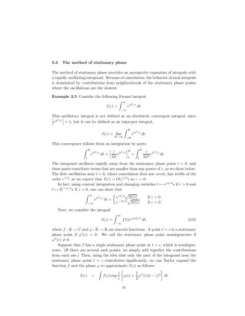
3.3 The method of stationary phase
The method of stationary phase provides an asymptotic expansion of integrals with
a rapidly oscillating integrand. Because of cancelation, the behavior of such integrals
is dominated by contributions from neighborhoods of the stationary phase points
where the oscillations are the slowest.
Example 3.5 Consider the following Fresnel integral
I(ε) =
∞
e
−∞
it2 /ε
dt.
This oscillatory integral is not defined as an absolutely convergent integral, since
eit2
/ε
= 1, but it can be defined as an improper integral,
R
I(ε) = lim e
R→∞ −R
it2 /ε
dt.
This convergence follows from an integration by parts:
R
e
1
it2 /ε
dt =
ε
2it eit2 /ε R +
1
R
1
ε
2it 2 eit2 /ε dt.
The integrand oscillates rapidly away from the stationary phase point t = 0, and
these parts contribute terms that are smaller than any power of ε, as we show below.
The first oscillation near t = 0, where cancelation does not occur, has width of the
order ε 1/2 , so we expect that I(ε) = O(ε 1/2 ) as ε → 0.
In fact, using contour integration and changing variables t ↦→ e iπ/4 s if ε > 0 and
t ↦→ E−iπ/4s if ε < 0, one can show that
∞
e it2
iπ/4
/ε e
dt =
2π|ε| if ε > 0
e−iπ/42π|ε| if ε < 0 .
−∞
Next, we consider the integral
I(ε) =
∞
−∞
f(t)e iϕ(t)/ε dt, (3.9)
where f : R → C and ϕ : R → R are smooth functions. A point t = c is a stationary
phase point if ϕ ′ (c) = 0. We call the stationary phase point nondegenerate if
ϕ ′′ (c) = 0.
Suppose that I has a single stationary phase point at t = c, which is nondegenerate.
(If there are several such points, we simply add together the contributions
from each one.) Then, using the idea that only the part of the integrand near the
stationary phase point t = c contributes significantly, we can Taylor expand the
function f and the phase ϕ to approximate I(ε) as follows:
I(ε) ∼
f(c) exp i
ϕ(c) +
ε
1
2 ϕ′′ (c)(t − c) 2
35
dt