Asymptotic Analysis and Singular Perturbation Theory

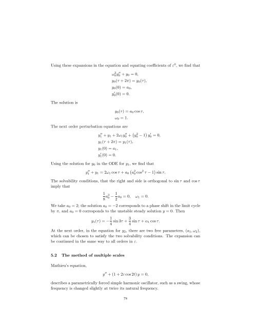
Using these expansions in the equation and equating coefficients of ε 0 , we find that
The solution is
ω 2 0y ′′
0 + y0 = 0,
y0(τ + 2π) = y0(τ),
y0(0) = a0,
y ′ 0(0) = 0.
y0(τ) = a0 cos τ,
ω0 = 1.
The next order perturbation equations are
y ′′
1 + y1 + 2ω1y ′′
0 + y 2 0 − 1 y ′ 0 = 0,
y1(τ + 2π) = y1(τ),
y1(0) = a1,
y ′ 1(0) = 0.
Using the solution for y0 in the ODE for y1, we find that
2
a0 cos 2 τ − 1 sin τ.
y ′′
1 + y1 = 2ω1 cos τ + a0
The solvability conditions, that the right and side is orthogonal to sin τ and cos τ
imply that
1
8 a30 − 1
2 a0 = 0, ω1 = 0.
We take a0 = 2; the solution a0 = −2 corresponds to a phase shift in the limit cycle
by π, and a0 = 0 corresponds to the unstable steady solution y = 0. Then
y1(τ) = − 1 3
sin 3τ +
4 4 sin τ + α1 cos τ.
At the next order, in the equation for y2, there are two free parameters, (a1, ω2),
which can be chosen to satisfy the two solvability conditions. The expansion can
be continued in the same way to all orders in ε.
5.2 The method of multiple scales
Mathieu’s equation,
y ′′ + (1 + 2ε cos 2t) y = 0,
describes a parametrically forced simple harmonic oscillator, such as a swing, whose
frequency is changed slightly at twice its natural frequency.
78