Asymptotic Analysis and Singular Perturbation Theory

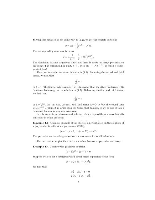
Solving this equation in the same way as (1.2), we get the nonzero solutions
y = ±1 − 1
2 ε1/2 + O(ε).
The corresponding solutions for x are
x = ± 1 1
− + O ε
ε1/2 2 1/2
.
The dominant balance argument illustrated here is useful in many perturbation
problems. The corresponding limit, ε → 0 with x(ε) = O(ε −1/2 ), is called a distinguished
limit.
There are two other two-term balances in (1.6). Balancing the second and third
terms, we find that
1
= 1
δ
or δ = 1. The first term is then O(ε), so it is smaller than the other two terms. This
dominant balance gives the solution in (1.5). Balancing the first and third terms,
we find that
ε
= 1,
δ3 or δ = ε 1/3 . In this case, the first and third terms are O(1), but the second term
is O(ε −1/3 ). Thus, it is larger than the terms that balance, so we do not obtain a
dominant balance or any new solutions.
In this example, no three-term dominant balance is possible as ε → 0, but this
can occur in other problems.
Example 1.3 A famous example of the effect of a perturbation on the solutions of
a polynomial is Wilkinson’s polynomial (1964),
(x − 1)(x − 2) . . . (x − 20) = εx 19 .
The perturbation has a large effect on the roots even for small values of ε.
The next two examples illustrate some other features of perturbation theory.
Example 1.4 Consider the quadratic equation
(1 − ε)x 2 − 2x + 1 = 0.
Suppose we look for a straightforward power series expansion of the form
We find that
x = x0 + εx1 + O(ε 2 ).
x 2 0 − 2x0 + 1 = 0,
2(x0 − 1)x1 = x 2 0.
5